Optimizing the profit from a complex cascade of hydroelectric
stations with recirculating water.
Andrei Korobeinikov∗ Alexander Kovacec † Mark McGuinness ‡ Marta Pascoal§ Ana Pereira ¶ S´onia Vilela k
Abstract. In modern reversible hydroelectric power stations it is possible
to reverse the turbine and pump water up from a downstream reservoir to an upstream one. This allows the use of the same volume of water repeatedly and was specifically developed for hydro-electric stations operating with in-sufficient water supply. Pumping water upstream is usually done at times of low demand for electricity, to build up reserves in order to be able to produce energy during peak hours, thus balancing the load and making a profit on the price difference.
In this paper, we consider a branched model for hydroelectric power stations interacting in a complex cascade arrangement. The goal of this study is to provide guidance in decision-making aimed at maximizing the profit. A detailed analysis is made of a simpler reservoir configuration, which indicates that even though the problem is nonlinear, a bang-bang type of control is optimal, where the power stations are operated at maximum rates of flow. Some simple relationships between price and timing of decisions are calculated directly. A numerical algorithm is also developed.
Keywords. optimization, hydroelectric power, branched cascade, re-versible turbines, case study
∗MACSI, Department of Mathematics and Statistics, University of Limerick, Limerick, Ireland, an-drei.korobeinikov@ul.ie
†Departamento de Matem´atica da FCTUC da Universidade de Coimbra, Apartado 3008, EC Universidade, 3001-454 Coimbra, Portugal
‡School of Mathematics, Statistics and Operations Research, Victoria University of Wellington, New Zealand,
Mark.McGuinness@vuw.ac.nz
§Departamento de Matemtica da FCTUC da Universidade de Coimbra, Apartado 3008, EC Universidade, 3001-454 Coimbra, Portugal, and Instituto de Engenharia de Sistemas e Computadores de Coimbra, Portugal,marta@mat.uc.pt
¶Instituto Polit´ecnico de Bragan¸ca, Portugal
Vilela
1
Introduction
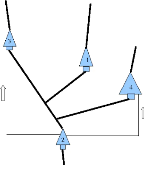
In modern reversible hydroelectric power stations it is possible to reverse the turbine to pump water up from a downstream reservoir to the upstream one. This is desirable when water supply is low as it allows reuse of the water. Water is usually pumped up at times of low demand and low price, to build up water reserves that can be used later to produce energy during times of high demand and high price, thus balancing the load and making a profit on the price difference. This, however, raises the question of when a turbine should be reversed to maximise profit. For a simple linear cascade composed of two hydroelectric stations that use the same stream the answer is reasonably straightforward. However, more complicated cascades, like the cascade depicted in Fig. 1, also exist and operate. Then there is also the question of which upstream reservoir is best to pump to. The cascade that is schematically depicted in Fig. 1 was presented as a case study by the Portuguese electricity and gas transmission supply operator, Redes Energ´eticas Nacionais, S.A. (REN), to the 69th European Study Group held at the University of Coimbra in Portugal in April 2009. The problem proposed was focussed on profit maximization when operating such a system, and how to decide which upstream reservoir to pump to, when there is a choice.
This cascade is composed of four hydroelectric plants that are enumerated as shown in Fig. 1. For this particular system, cascades are formed by plants 2&3, 1&2, and 2&4. In cascades 2&3 and 2&4, water from the reservoir of plant 2 can be pumped back to plants 3 and 4, as indicated by the additional arrows in Figure. Pumping is done via reversible turbines at plants 3 and 4, respectively.
Figure 1: Schematic representation of a cascade of four hydro-electric stations.
Relevant main parts of a typical hydroelectric plant, or a power station, depicted in Figure 2, are: (i) the reservoir with its current water content (volume)V(t), measured inm3 and represented
through a turbine at an instant tis denoted byq(t).
Figure 2: Representation of a hydroelectric plant.
In a full model of a hydroelectric system, the incoming flows influence the water volumes, which determine the water levels, which in turn determine the heads, which influence the outgoing flows, which influence the reservoir levels as well as the energy sales, and these together with the price determine the profit. It is thus clear that in a full formulation the problem of optimizing the profit is a complex nonlinear stochastic problem. Similar or related problems have been studied for the past few decades. Even though various approaches to this problem have been developed, in general, due to complexity of the problem, these are mathematically complex and are usually perceived to be difficult to implement in practice. Very few operating hydroelectric sites actually use optimization methods for controlling the flows. Furthermore, certain aspects of the problem, like rain, evaporation, demand or pricing, are uncertain or stochastic by their nature. Thus, the methods available in the literature focus on deterministic models, where those aspects are only implicitly stochastic, as well as on stochastic models, where these uncertainties are explicitly taken into account. Some of the techniques involved include linear and nonlinear programming, network flow optimization, dynamic programming and stochastic optimal control. An extensive survey of methods for optimal operation of multi-reservoir systems can be found in the paper by Labadie [3] that was published in 2004.
A goal for this study was optimizing the profit from operating a complex cascade of hydroelectric plants, by developing an optimal strategy for shifting a turbine from one mode of operation to the other. This study focusses on the particular system of hydro-electric plants proposed by REN and depicted in Fig. 1. However, where possible, we also consider a more general system aiming to inform a general approach that may be applied to other systems.
2
Notation and Mathematical formulation
Here we define our notation and provide formulae for the specific case of a system of four hydoelectric power stations as depicted in Fig. 1. Below we use the same generic notation for all four plants, which are distinguished by subscripts i= 1, ...,4.
Specified constants:
• initial and minimal water volumes in reservoirs,Vin
i andVi0, respectively;
• nominal, minimal and maximal water levels (metres above sea level) in reservoirs, Zi0, Zimin and Zmax
Vilela • nominal flowrates and heads qi0,h0i;
• other constants: αi,βi,ζi,ξ,µi,φi. Specified functions of time:
• inflows from rivers Ii(t);
• the market price of 1 MWh price(t).
Calculated functions of time:
• water volumes in reservoirsVi(t);
• water levels in reservoirs Zi(t);
• heads (differences in water levels) hi(t);
• head losses ∆hi(t).
Sought-for functions of time:
• flow ratesqi(t).
Here we adopt the convention that pumping water upstream corresponds to qi(t) < 0, and
‘turbining’ (producing electricity) corresponds to qi(t) > 0. Where appropriate, we also use the
notation qP and qT for the rates of pumping and turbining, respectively; then our convention is
thatqP and qT are non-negative.
The following expressions relate the elements of the system. They arise directly from the physics of water flow and electricity generation, and simply state that water volume is conserved, that water level varies according to flows in and out of a reservoir, that flowrate down a pipe varies as the square root of the height difference (pressure difference) driving the flow, and that the power produced is proportional to the height difference and flowrate (force times velocity).
The integrals Rt
0f should be interpreted as
Rt
0f(u)du. Also, for the sake of simplicity, the
dependence of functions on tis not always explicitly shown. Equations
V1(t) = V1in+
Z t
0
(I1−q1),
V2(t) = V2in+
Z t
0
(I2−q2+q1+q3+q4),
V3(t) = V3in+
Z t
0
(I3−q3),
V4(t) = V4in+
Z t
0
(I4−q4)
(1)
For instance, the most complicated volume functionV2is obtained as follows. The water volume
in reservoir 2 as a function of time is determined by the initial volume V2in plus the cumulative volumes (integrals) of all inwards and outwards fluxes from the momentt= 0 to the instantt. The inflows to the reservoir are comprised of the influx from an ‘external river’ (due to precipitation, for example) given byI2(t), and the outflowsq1, q3, q4 from reservoirs 1, 3, and 4. The outflow from
reservoir 2 is q2. Note that q3, q4 can be both positive and negative (for turbining and pumping,
respectively), and that when negative these fluxes also cause reduction of water volume in reservoir 2. The formulae for volumes Vi,i= 1,3,4, are obtained analogously.
Water level is a function of reservoir volume, given by the formulae Z1(t) = Z10+α1(V1(t)−V10)β1,
Z2(t) = Z20+α2(V2(t)−V20)β2,
Z3(t) = Z30+α3(V3(t)−V30)β3,
Z4(t) = Z40+α4(V4(t)−V40)β4
(2)
where the constants αi, βi, Zi0, Vi0 are fitted to each reservoir.
The water head (the height difference) that drives each turbine is given by the difference in reservoir heights above and below the turbine as follows:
h1(t) = Z1(t)−Z2(t),
h2(t) = Z2(t)−ξ,
h3(t) = Z3(t)−Z2(t),
h4(t) = Z4(t)−Z2(t).
(3)
The constant ξ for reservoir 2 is due to the fact that this reservoir is the lowest downstream in the chain of the reservoirs, and hence the outflow from this particular reservoir goes to the sea at atmospheric pressure rather than to another reservoir.
The water level Z of a reservoir has upper and lower limits that arise from technical or envi-ronmental considerations — for example, an empty reservoir has no water in it, and a full reservoir cannot go any higher in water level. These limits are given by the following formulae:
Z1min≤ Z1(t) ≤Z1max,
Zmin
2 ≤ Z2(t) ≤Z2max,
Z3min≤ Z3(t) ≤Z3max,
Zmin
4 ≤ Z4(t) ≤Z4max.
(4)
The flow through a turbine is limited by its maximal value q0qh
h0, where q0, h0 are constants
Vilela
recalling that, with our definition,q is negative when pumping: 0≤ q1(t) ≤q01
h
1(t)
h0 1
1/2 ,
0≤ q2(t) ≤q02
h2(t)
h0 2
1/2 ,
−q0
3+ζ3(h3(t)−h30)≤ q3(t) ≤q03
h3(t)
h0 3
1/2 ,
−q0
4+ζ4(h4(t)−h30)≤ q4(t) ≤q04
h
4(t)
h0 4
1/2 .
(5)
Finally, by varying the control variablesqi(t), we can change the net profit. At a given moment,
each plant either turbines producing revenue, or pumps water upstream originating expenses, or the system is shut and there is zero flow. We combine the formulae for the value of power output and the expense of pumping in the piecewise functionr(t):
ri(t) := (
9.8qi(hi(t)−∆hTi (t))µiT(1−φi) if qi(t)≥0,
9.8qi(hi(t) + ∆hPi (t))µP 1
i(1−φi) if qi(t)<0.
(6)
Here
∆hTi (t) = ∆h0iT
qi(t)
q0T i
2
represents friction losses when turbining, and
∆hPi (t) = ∆h0iP
qi(t)
q0P i
2
is due to frictional losses when pumping; both these values are expressed as a head loss. The nominal values ∆h0iT, q0iT, ∆h0iP and q0iP are constants specific to each turbine; the parameters µT
i ≈0.95 and 1/µPi ≈1.1 represent efficiencies of turbines in electricity production mode (T) and
pumping mode (P), respectively.
The market price of energy per megawatt is price(t). The objective of the process is maximizing the profit, defined as
Profit = Z 1 0 price(t)· 4 X i=1
ri(t)dt.
The profit is to be maximized subject to the constraints listed in equations (1)–(6).
3
Energy Considerations
3.1 Limited Water
Here we consider the benefit of pumping a unit volume of water in unit time (soq=−1) up through a head difference of h at a time when the cost isC, and then later turbining that unit volume (so that q = 1) when the price of electricity is P. The profit is proportional to (P −C)h according to the formulae above. In this case, it is clearly better to pump to the higher reservoir, if there are no other considerations such as that reservoir being full. This corresponds to maximising the potential energy of the unit of water.
3.2 Limited Time
Now consider the benefit of pumping at maximum flowrate qP (which depends on head) for a
fixed small time when costs are low at the value C, then turbining water at maximum flowrate qT for the same fixed small time when values are high at P. Then the net profit takes the form AP qTh−BCqPh, with constant A,B. That is, net profit is
AP h3/2−BC(h−Dh2),
where D is a constant. This means the net profit depends on the difference between a curve varying ash3/2 and a curve with the shape of an upside-down quadratic inh. Curves with these shapes are
sketched in Fig.3, and again indicate that it is advantageous (for large enough heads) to pump to the higher reservoir, if the choice has to be made and if other constraints do not prevent this.
Figure 3: A sketch of two curves, the solid line ofh3/2
, and the dashed line ofh−h2
Vilela
4
A Simple Model
We now focus on a simplified system by considering a linear cascade composed of a plant and a reservoir downstream (see Fig. 4). The purpose of this is to reduce the system to one that is amenable to some careful analysis, while still retaining interesting behaviour.
For the sake of simplicity, we assume there is no influx of water into the system from any external source, that is I2 =I3 = 0. Furthermore, we assume that the downstream reservoir (reservoir 2 in
Fig. 4) has no turbine, and hence there is no flux from it. That is we assume thatq2 = 0 always,
and we will use notation q forq3. We also prevent turbine 3 from pumping, soq ≥0.
Note that the formulae Z = Z0 +α(V −V0)β, with α, β > 0, h = Z
3−Z2, imply that the
functions Zi are increasing with Vi, and hence bounds for Zi translate to bounds for Vi. Further,
h as a function ofV2, V3 is continuous, decreasing with V2, and increasing with V3.
Figure 4: Scheme of hydroelectric cascade with two reser-voirs.
Thus, our model is constrained as follows: V3(t) =V3in+
Z t
0
−q ≥ 0, (7)
V2(t) =V2in+
Z t
0
q ≤ V2max. (8) There exists a continuous functionh(x, y), decreasing inxand increasing inyso thath(V2(t), V3(t))
gives the head. We use the notation h(t) =h(V2(t), V3(t)). The bounds on the flow are given by
0≤q(t)≤q0
s h(t)
h0
, (9)
and the simplified function to maximize is the profit Profit =
Z 1
0
p(t)q(t)h(t)dt .
Herep(t) is the price of electricity, and all functions are ultimately functions of timet, a parameter often suppressed for the sake of simplicity.
w is the change (fromq to ˆq). The change w is said to be feasible if the constraints (7)–(9) still hold after its application. The volume functions associated with ˆq are
ˆ
V3(t) =V3(t)−
Z t
0
w, Vˆ2(t) =V2(t) +
Z t
0
w.
Here we use the notation ˆh(t) = h( ˆV2(t),Vˆ3(t)), and hereafter the expression ‘for small . . . ’ will
mean ‘there exists an ǫ >0 such that for all . . . smaller than ǫwe have . . . ’.
Lemma 1 Assume q(t) is a continuous function, andt0 a point where conditions (7), (8) and (9)
are satisfied with strict inequalities. Then there exist small continuous feasible changes w(t) with
w(t0)6= 0. Such changes can be chosen of arbitrarily small support and such that
R1
0 w= 0.
Proof. Since by (9), q ≥ 0, then V3 is non increasing, and V2 is nondecreasing. Hence (7), (8)
are equivalent to V3(1) ≥ 0 and V2(1) ≤ V2max. By hypothesis, V3(t0) > 0, V2(t0) < V2max and
0< q(t0)< q0
q h
h0. Continuity of the functions involved implies that there is an opent0-centered
intervalI such that these inequalities still hold for allt∈I in place of t0. Scaling the sin function
(for which R2π
0 sint dt = 0), we get a continuous function w of arbitrarily small | · |∞-norm, such
that supp(w) ⊆ I, and R Iw =
R1
0 w = 0. The | · |∞-continuity of integrals implies that, for all
small enough w(t), ˆV3(t), ˆV2(t) satisfy inequalities (8) and (9), and that ˆVi|Ic = Vi|Ic, i = 2,3
holds. Therefore, we also have h|Ic = ˆh|Ic. The continuity of the head function in both variables
guarantees that for small w(t), the function ˆh(t) has only small deviation fromh(t).
Proposition 1 Assume we subject q(t) to a change w(t) with supp(w) ⊆I and R Iw=
R1
0 w= 0.
Then the change in profit is given by
Z
I
p(t)(wˆh+q(ˆh−h))dt.
Proof. We have ˆqˆh= (q+w)(h+ ˆh−h) =qh+q(ˆh−h) +wˆh, and therefore ˆ
Profit = Z 1
0
p(t)ˆqˆh =
Z 1
0
p(t)qh+ Z 1
0
p(t)(q(ˆh−h) +wˆh) = Profit +
Z
I
p(t)(wˆh+q(ˆh−h))dt.
The justification for the shortening of the interval of integration is that supp(w)⊆I andh|Ic= ˆh|Ic
by a similar behaviour for the ˆV with regards to V (see proof of Lemma 1).
We can take these calculations a step further. We recall an instance of Taylor’s theorem which states that if f is a twice differentiable function on a x0 = (x0, y0)-centered open ball in IR2 of
radius larger than the norm ofh= (h1, h2), then for some ϑ, 0≤ϑ≤1,
f(x0+h) =f(x0) +∂1f(x0)h1+∂2f(x0)h2+
1 2
2
X
j,k=1
Vilela
Here ∂j denotes the derivative with regards to the jth variable, j = 1,2, and underlined letters
denote 2-tuples. Now, recalling that ˆh(t) =h(V2(t) +R0tw, V3(t)−R0tw), fixing tand applying the
Taylor formula to the 2-variable h, we get ˆ
h(t) =h(t) + (∂1h−∂2h)(V1, V2)
Z t 0 w+ Z t 0 w 2 R(t), where
R(t) = 1 2
2
X
i,j=1
∂i∂jh(V2+ϑ, V3−ϑ)(−1)i+j.
Substituting this into the expression for Profit, and using some simplification of the notation, weˆ find
ˆ
Profit = Profit +R Ip(t)
h+ (∂1h−∂2h)R0tw+ (R0tw)2R(t)
w+
(∂1h−∂2h)
Rt
0w+ (
Rt
0w)2R(t)
q.
Lemma 2 Let I be an interval such that the functionsis strictly monotone inI. Then there exists
a differentiable function w:I →IR such that
1. R
Iw= 0 and
2. R
Is·w >0.
Proof. After rescaling we may take the interval to be [0,2π]. Then functionw(t) = sintsatisfies (7). Furthermore,
Z 2π
0
s(t) sint dt = Z π
0
s(t) sint dt+ Z π
0
s(t+π) sin(t+π) dt =
Z π
0
s(t) sint−s(t+π) sint dt =
Z π
0
(s(t)−s(t+π)) sint dt
holds. Moreover, sin|[0, π]≥0, and hence for strictly decreasing function s s(t) > s(t+π) holds, and the integral is positive. Ifsis increasing, the same argument works by replacing sin with−sin.
If h is constant, we have (∂1h−∂2h)≡0 and R(t)≡0, and then this formula simplifies to
ˆ
Profit = Profit + Z
I
p(t)h(t)w(t).
In this case we can state the following corollary.
Corollary 1 If h is constant and there exists a moment t0 where all inequalities (7), (8), (9) are
strictly satisfied, and in a neighbourhood of which p(t) is strictly increasing or decreasing, then the
This corollary can be translated as follows: if q is the current flow, and there is a moment t0
such that at this moment
• the reservoir 3 is nonempty, and the reservoir 2 is not full;
• the price is strictly dropping or increasing in some neighbourhood oft0; and
• the turbining is neither zero nor maximal,
then the flow q can be changed to one with a larger Profit.
Note that up to this point we have not considered the optimal solution. In fact, in the class of continuous functions there does not seem to exist an optimal solution; all solutions that can be improved upon. This suggests that the optimal solutions may be piecewise continuous. Since for a constant h, maximising R1
0 p(t)q(t)h(t)dt is equivalent to maximising
R1
0 p(t)q(t)dt, we consider
now this latter problem in more detail. We replace the conservation law of the previous problem, namely V2+V3 =V2in+V3in, with
R1
0 q =c. This can be interpreted, for example, as that in the
interval [0,1] the difference between turbining and pumping leads to a (possibly negative) net excess c in reservoir 3 without violating the volume inequality applying there. Therefore, the following theorem applies to a more general situation where pumping is allowed. From the proof an optimal method for choosing when to pump and when to turbine can be deduced.
Theorem 1 Letp: [0,1]→IR≥0be a piecewise strictly monotone continuous function, representing
the price of electricity, price(t). Then, if in the family of piecewise continuous functionsPˇ on[0,1]
there is an optimal solution to the problem
max Z 1
0
p(t)q(t),
such that
Z 1
0
q(t)dt=c anda≤q(t)≤b hold, then this solution can be found constructively.
Proof. Since p : [0,1] → IR≥0 is continuous, it is measurable and bounded; that is, for each
e ∈ IR, the set E(e) = p−1([e,∞[) is a Lebesgue measurable set, and the real valued function IR≥0 ∋e7→l λ(E(e)) is decreasing, hasl(0) = 1, and is of compact support. Piecewise monotonicity
guarantees furthermore that l is continuous. Assume now the existence of aq∈Pˇ that is optimal among the feasible functions in ˇP . Ifa=b, thenq is necessarily constant and equal toa, and thus the unique feasible and hence optimal function in ˇP. So we can henceforth assume a < b. Then there exists a unique λ0 ∈]0,1[ such that c = λ0b+ (1−λ0)a. By the properties of l, we find a
uniquee. such thatl(e.) =λ0 holds. From now on letE =E(e.). We claim that if there exists an
optimal functionq, it is given by
q(t) = (
Vilela
To see this, note firstly that clearlyq ∈Pˇ,q satisfies the bounds, and Z 1
0
q(t)dt= Z
E
q dt+ Z
Ec
q dt=λ(E)b+ (1−λ(E))a=λ0b+ (1−λ0)a=c
holds. Henceq is feasible. Next we show that every feasible function ˇq ∈Pˇwith ˇq 6=qis improvable (and hence not optimal). Take such a function ˇq, and assume that ˇq|E = q|E holds. Then there exists a t0 ∈ Ec such that ˇq(t0) > q(t0) = a holds. By piecewise continuity of ˇq, we get that
R
Ecq dt >ˇ R
Ecq dtholds. From here we infer that R1
0 q dtˇ =
R
Ecq dtˇ + R
Eq dt >ˇ R1
0 q dt=c, that is
a contradiction. Therefore, ˇq|E6=q|E must hold. Similarly one can show that ˇq|Ec 6=q|Ec holds. Consequently, there exist t0, t1 and intervals I0, I1 of the same length, satisfying
t0 ∈I¯0, I0 ⊆Ec, t1 ∈I¯1, I1 ⊆E,
and ˇq|I0 > a, ˇq|I2< b. Now define the function
ˆ q(t) = ˇ
q if t6∈I0∪I1,
ˇ
q−δ if t∈I0,
ˇ
q+δ if t∈I1.
For small enough δ > 0, ˆq ∈ Pˇ is feasible, and observing that p|E > e. > p|Ec holds almost
everywhere (by strict monotonicity), we get Z 1
0
pq dtˆ = Z
[0,1]
pˇq dt+δ Z
I1
p dt−
Z I0 p dt > Z 1 0
pq dt.ˇ
This shows that ˆq improves ˇq and completes the proof.
This Theorem claims, in the Corollary above, that if there exists an optimal control q(t), then this optimal control is necessarily a bang-bang process: in order to maximize the profit it requires either pumping at the maximum possible rate, or turbining at the maximum flow. Note that the assumption that p(t) is strictly monotone is not very restrictive: price may be sampled and re-ordered to ensure that it is at least monotone if not strictly so.
Example 1 Assume that we have a price curve as shown in Fig.5, and the constraints−1≤q ≤2
and R1
0 q dt= 1. The problem is maximizing
R1
0 pq dt under these constraints.
Solution: From the equationλ0·2 + (1−λ0)·(−1) = 1 we find thatλ0 = 2/3. Draw a horizontal
line l so that the points (a union of the intervals) in [0,1] obtained by projecting the part of the curve lying above l has measure 2/3. Turbine in the intervals formed by that set of points at rate 2 and pump at rate 1 in the remaining intervals.
The discrete analogue to the above theorem reads as follows.
Theorem 2 Assume p1, p2, . . . , pn are positive real numbers. Then the problem
max
n X
i
0 5 10 15 20 25 35
40 45 50 55 60
Figure 5: The price curve used in our example, showing the
price of electricity during a winter’s day.
such that Pn
i=1qi =c and a ≤qi ≤b hold, has a solution such that all but at most one of the qi
are equal to aor b.
This theorem can be proved similarly to the previous theorem, or by using linear programming. Here the existence of an optimal solution can be readily guaranteed. In Section 6 we give an illustration of the theorem by means of a computational implementation.
5
More Complex Models
We now consider a complex cascade of n hydro-electric stations (Fig. 1). We assume that the result of previous Section can be extended to this more general case, so that to maximize profit a turbine must be operated at maximum flowrate for both regimes, turbining and pumping. That is, we assume that the control of the turbine and shifting from turbining to pumping is a bang-bang process.
This is a serious assumption, but is in the spirit of a heuristic approach to solving optimization problems that cannot be solved in any other way, even numerically [3], since the parameter space to be searched is prohibitively large. Note that bang-bang solutions are optimal when the objective function is linear in the control variable (here the flowrate), according to Pontryagin’s minimum principle [1]. This corresponds to linearizing our objective function in the flowrates.
We also assume that the price of electricity is known in advance for the operational time interval. We consider separately three possible cases, namely:
Vilela
2. There is not enough water for continuous operation of the stations with water recirculation; redistribution of water between these stations can be needed in this case (Small reservoirs
case).
3. There is not enough water for continuous operation in stations with water recirculation, but there is a reserve of water in the reservoirs of “downstream only” stations; optimizing the usage of this water (with possible redistribution of this reserve for continuous operation of the stations with recirculation) is the question in this case (Not enough watercase).
5.1 Case 1: Large Reservoirs
In this case, we assume that all reservoirs have enough water and enough empty space for continuous operation, that is, that the bounds on reservoir size never act to limit electricity production or pumping of water.
We consider operation of a system ofnhydro-electric stations on the time interval [0, T] (where T may be 24 hours, or a week, or any other sensible period of time). We assume that for each of these stations the operational time interval [0, T] is divided into three operational states as follows:
1. on the interval TT
i = [ai, bi] the ith station produces electric energy with the power Pi(t)
releasing water downstream with the flow rateqiT(t);
2. on the interval TiP = [ci, di] the ith station produces a reserve of water that can be used
later, by pumping water upstream at the flow rate qPi (t), and consuming energy to operate the turbine in pumping mode with the powerC(t);
3. outside of these two intervals there is no flow. The intervals do not overlap, and without loss of generality we will assume the second interval follows the first.
For each station, profit is
Z bi
ai
p(t)Pi(t)dt− Z di
ci
p(t)Ci(t)dt,
and the total profit of the system of stations over the operational interval is U(ai, bi, ci, di) =
X
i Z bi
ai
p(t)Pi(t)dt− Z di
ci
p(t)Ci(t)dt
.
Here, p(t) is the price of electricity that we assume known in advance, and the powers P(t) and C(t) are (dropping the subscripts)
P(t) =gµTqT(t)·(h(t)−∆hT)(1−φ) and
C(t) =g 1 µPq
respectively. Here g is gravitational acceleration, g= 9.8 m.s−2; h(t) is the head of a station (the difference between the levels of the upper and lower reservoirs), ∆hP and ∆hT represent the losses due to drag and friction, represented here as head losses, ∆hP,T = ∆hP,T0 (qP,T(t)/qP,T0 )2 and µP,T and φare constants.
In this subsection we assume that each station with water recirculation has sufficient reserve of water for continuous operation, and that the ith reservoir has an excess of water ∆Vi over the
time period (perhaps from precipitation), that is to be discarded from recirculation; ∆Vi can be
negative when we decide to store some extra water into the reservoir. That is, for each station with water recirculation we have the constraint
Z bi
ai
qTi (t)dt−
Z di
ci
qPi (t)dt= ∆Vi. (10)
Guided in a heuristic manner by the results of the previous section, and noting Labadie’s comment [3] that heuristic methods are usually required, we assume that for both modes, pumping water and producing energy, operating the turbine at the maximum possible flow rate maximizes profit. Then we can formulate the problem of maximizing profit as an extremum problem with Lagrange multipliers and consider the functional
U(ai, bi, ci, di) = X
i
Z bi
ai
p(t)Pi(t)dt− Z di
ci
p(t)Ci(t)dt
+ X
i
λi Z bi
ai
qTi (t)dt−
Z di
ci
qiP(t)dt−∆Vi
.
Extrema occur at critical points, which are either boundary values or obey the following set of equations:
∂U ∂ai
= −p(ai)Pi(ai)−λiqiT(ai) = 0,
∂U ∂bi
= p(bi)Pi(bi) +λiqiT(bi) = 0,
∂U ∂ci
= p(ci)Ci(ci) +λiqPi (ci) = 0, (11)
∂U ∂di
= −p(di)Ci(di)−λiqiP(di) = 0.
It is remarkable that in this case these equations are independent for each of the stations. According to (11), the equalities
p(ai)Pi(ai)
qTi (ai)
= p(bi)Pi(bi) qTi (bi)
= p(ci)Ci(ci) qiP(ci)
= p(di)Ci(di) qPi (di)
=−λi (12)
hold for each reservoir. The valuesQT
i (t) = p(t)P
i(t)
qT i (t)
andQP
i (t) = p(t)C
i(t)
qP i (t)
Vilela
trades in water. We further refer to the values QPi (t) and QTi (t) as effective prices of water, for pumping and turbining respectively.
Note that for a given reservoir and at a given moment the prices of water will be different for turbining and pumping, that is QT
i(t)6=QPi (t), and hence we apply the indexesT, P for turbining
and pumping, respectively. This difference is mostly due to the fact that energy production is not a perfect process, and only a fraction of the potential energy that is stored by water can be turned into electric energy. In general,QT
i (t)< QPi (t) holds. Indeed, if
P(t) =gµTqT(t)·(h(t)−∆hT)(1−φ) and
C(t) =g 1 µPq
P(t)·(h(t) + ∆hP),
then the effective water prices are
QT(t) =gµTp(t)·(h(t)−∆hT)(1−φ) and
QP(t) =g 1
µPp(t)·(h(t) + ∆h P),
respectively. It is easy to see that even in the case µT(1−φ) = µ1P =µ, the price difference is ∆Q=QP(t)−QT(t) =g µ p(t)·(∆hP + ∆hT)>0,
which is due to the head loss terms. Furthermore, due to different heads and differences in operating efficiencies, for two different stations the same volume of water can be turned into different amounts of electric energy. Therefore, for a given moment of time the pricesQTi (t) and QPi (t) for different reservoirs are different.
The equalities (12) literally state that in order to maximize the profit, each process, turbining or pumping, must start and end at the moments when the effective price of water is equal. That is, the conditions
QTi (ai) =QTi (bi) =QPi (ci) =QPi (di) (13)
must hold for each reservoir.
The length of each regime, turbining, TT
i =bi−ai, and pumping, TiP =di−ci, can be found
from the water balance constraint. By the Lagrangian minimax principle, nequalities ∂U
∂λi
= Z bi
ai
qTi (t)dt−
Z di
ci
qiP(t)dt−∆Vi = 0
an assumption appears to be accurate for reasonably short time intervals that are of order of a few hours.) Under this assumption,
Z bi
ai
qiT(t)dt=qTi (bi−ai),
Z di
ci
qiP(t)dt=qiP(di−ci),
and henceqT
i TiT−qPi TiP = ∆Vi. That is, when there is no excess of water to discard from circulation,
∆V = 0, and the lengths of these two regimes are simply inversely proportional to the flow rates: qP i qT i = T T i TP i .
We have to comment, however, that, due to the fact that QTi (t) 6= QiP(t) (QTi (t) < QPi (t)), we cannot put TT +TP = T even if shifting a turbine from energy producing to pumping and
back were possible. (Generally this shifting requires some time.) By (13), QTi (bi) = QPi (ci) must
hold at the moments of the end of turbining mode, t=bi, and the begin of pumping, t=ci. But
QT
i (bi) < QPi (bi) and QTi (ci)< QPi (ci). That is, bi 6=ci, and there is a time lag between stopping
turbining at t=bi and beginning pumping att=ci.
5.2 Case 2: Small Reservoirs
We assume now that the stock of water is not sufficient to maintain continuous operation of those stations that can recycle water. In this case the available water must be re-distributed between the reservoirs with the aim of maximizing profit. We assume that there is no excess of water, that is ∆V = 0, and hence the water balance constraint is
X
i
Z bi
ai
qiT(t)dt−
Z di
ci
qPi (t)dt
= 0. (14)
The problem is re-formulated accordingly as U(ai, bi, ci, di) =
X
i Z bi
ai
p(t)Pi(t)dt− Z di
ci
p(t)Ci(t)dt
+ λX
i
Z bi
ai
qiT(t)dt−
Z di
ci
qPi (t)dt
.
As before, we are looking for the values ofai, bi, ci, dithat maximize this functional. Internal critical
points occur when
∂U ∂ai
= −p(ai)Pi(ai)−λqTi (ai) = 0,
∂U ∂bi
= p(bi)Pi(bi) +λqTi (bi) = 0,
∂U ∂ci
= p(ci)Ci(ci) +λqiP(ci) = 0, (15)
∂U ∂di
Vilela Hence,
p(ai)Pi(ai)
qiT(ai)
= p(bi)Pi(bi) qiT(bi)
= p(ci)Ci(ci) qPi (ci)
= p(di)Ci(di) qiP(di)
=−λ (16)
hold for each reservoir.
Note that in contrast with the previous subsection, here λ is the same for all reservoirs with water recirculation. Using the idea of effective price of water from the previous subsection, we can rewrite (16) as
QTi (ai) =QTi (bi) =QPi (ci) =QPi (di) =−λ.
The major difference with the earlier case is the fact that here for all stations with water recycling every mode of operating, that is turbining or pumping, should start at the same level of the effective price of water. We note that same price for different reservoirs does not mean the same moment of time, because the cost of pumping and the value of turbining may differ for different reservoirs. For example, if we have just two reservoirs i= 1,2 with water recycling, then
QT1(a1) =QT2(a2) =QT1(b1) =QT2(b2) =QP1(c1) =QP2(c2) =QP1(d1) =QP2(d2)
must hold. These equalities gives an idea how the total water stocks should be redistributed between the stations with water recirculating in the case when water stocks are insufficient to provide continuous operation of these stations. The condition
QT1(a1) =QT2(a2) =QT1(b1) =QT2(b2)
implies
µT1p(a1)·(h1(a1)−∆hT1) = µT2p(a2)·(h2(a2)−∆hT2) = (17)
=µT1p(b1)·(h1(b1)−∆hT1) = µT2p(b2)·(h2(b2)−∆hT2).
Assuming that both stations use the same technology and are similar in characteristics, and hence µT
1 ≈µT2, and neglecting by ∆hT1,∆hT2, we obtain the conditions
p(a1)·h1(a1) =p(a2)·h2(a2)
and
p(b1)·h1(b1) =p(b2)·h2(b2).
That is, for two stations, switching between pumping and turbining should occur at times a1, a2 (or c1, c2, respectively) such that the ratios of the energy prices at these times are inversely
proportional to the ratios of the heads: p(a1)
p(a2)
= h2(a2) h1(a1)
, p(b1) p(b2)
= h2(b2) h1(b1)
The assumptionµT1 ≈µT2 and the neglecting of ∆hT1,∆hT2 are not necessary here: it is easy to see from (17) that optimal times to switch between pumping and turbining satisfy
p(a1)
p(a2)
= µ
T
2 ·(h2(a2)−∆hT2)
µT
1 ·(h1(a1)−∆hT1)
, p(b1) p(b2)
= µ
T
2 ·(h2(b2)−∆hT2)
µT
1 ·(h1(b1)−∆hT1)
.
If we have more that two stations with water recirculating in the system, then these conditions must hold for every possible pair of stations.
These conditions also imply that a reservoir with a larger head should start producing electricity at a lower price; this suggests that such a reservoir can start earlier in a rising market, and continue longer in a falling price market, than a reservoir with a smaller head, echoing earlier simple analysis of the relative value of water in different reservoirs in section (3).
As earlier, the water balance constraint X
i Z bi
ai
qiT(t)dt=X
i Z di
ci
qPi (t)dt
must also hold in this case. This constraint can be obtained from the condition ∂U∂λ = 0.
5.3 Case 3: Not enough water
Let us assume now that the stations with water recirculation do not have sufficient reserve of water to maintain continuous operation, and that there are a few stations that are unable to pump water upwards. The latter have some reserve of water that can be used. The question is how this reserve can be used optimally. That is, should we flush this reserve down as soon as possible to provide enough water for continuous operation of a station with water recirculation, or should we apply a different strategy.
In this case it appears that if this reserve or a part of it can be re-distributed for the stations with water recirculation, then it makes sense to flush downstream the volume of water that is sufficient to provide uninterrupted operation of the stations with recirculation: the profit that was missed initially will be substantially replenished after a few recurrent operating cycles of the stations with water recycling.
6
Numerical Solutions
The numerical procedure and solutions presented in this section are intended to illustrate the theoretical ideas discussed in earlier sections.
Vilela
problem. In this Section we indicate a numerical method that utilizes a discretized model of the problem.
We assume that the time period is divided into m subperiods, and that the electricity price is constant on each of these periods. Then the objective function is given by
U =
m X
j=1
pj
4
X
i=1
rij,
where
• pricepj is the market cost of electricity at thejth interval, j= 1, . . . , m;
• power rij = (
9.8qij(hij −∆hij)µi(1−φi), if qij ≥0, i= 1, . . . ,4 ;
9.8qij(hij + ∆hij)/µi, if qij <0, i= 3,4.
The nominal point of each reservoir, (qi0, hi0), is assumed to be given. Parameters µi and φi are
also known and are related to each power station’s efficiency. The powerrij depends on the head
hij and the water flux qij in the ith reservoir on the jth time subinterval, where i = 1, . . . ,4,
j = 1, . . . , m. (Please note that here we again assume that the flux q is positive when the plant is turbining and negative when the plant is pumping water up, and hence we use the notation q rather thenqT and qP for both regimes of operating.)
The flow rates are subject to constraints. Thus, for the particular system depicted in Fig. 1, the flow rates are limited by the following constraints:
0≤ qij ≤qij−1
s hij
hij−1
, i= 1,2, j= 1, . . . , m.
−qij−1+ζi(hij −hi0)≤ qij ≤qij−1
s hij
hij−1
, i= 3,4, j= 1, . . . , m.
For the discrete-time model, the relationships between the heads, water levels, water volumes and the fluxes of the reservoirs for the particular cascade depicted in Fig. 1are:
hij = Zij −Z2j, i= 1,3,4, j= 1, . . . , m;
h2j = Z2j−ξ, j= 1, . . . , m;
V2j = V2j−1+I2j +q1j+q3j+q4j−q2j, j = 1, . . . , m;
Vij = Vij−1+Iij −qij, i= 1,3,4, j = 1, . . . , m;
Zij = Zij−1+αi(Vij−Vij−1)βi, i= 1, . . . ,4, j = 1, . . . , m.
Here ξ denotes sea level; Iij denotes natural water influx into the ith reservoir on the jth
subinterval; Vij denotes the volume of water in the ith reservoir on the jth subinterval; αi and βi
The initial volumes Vi0 are assumed to be known for each of the reservoirs. There are lower and
upper bounds on the volume of water each reservoir can store,
Vimin≤Vij ≤Vimax, i= 1, . . . ,4, j = 1, . . . , m,
whereVmin
i and Vimax denote the bounds given for theith reservoir.
In this formulation, the problem can, in principle, be solved numerically by a solver for non-linear optimization, or, if the objective function and the non-non-linear constraints are non-linearized, by a solver for linear programming.
6.1 Computational experiments
For the particular case of a single hydro-electric plant, with linear objective function and constraints, we have carried out numerical experiments using the numerical method that is described above. For computation we use a 24-hour time interval, divided into 24 subintervals, and the price of electricity given in Fig. 5. That is, we attempted to numerically find the set of constants qj (j = 1, . . . ,24)
which maximize the objective function
max
24
X
j=1
pjqj,
subject of constraints
24
X
j=1
qj =θ, −2≤qj ≤10.
Figure6shows the results of computations obtained forθ= 100 by a Matlab package for nonlinear optimisation linprog(Fig. a), and by the simplex method with CPLEX [2] (Fig. b).
0 5 10 15 20 25
−2 0 2 4 6 8 10
0 5 10 15 20 25
−2 0 2 4 6 8 10
(a) Package linprogof Matlab (b) Simplex method of CPLEX Figure 6: Solution of the linear problem with θ= 100
Vilela
These comparatively simple tests illustrate nicely the theoretical results, suggesting that bang-bang values forq are optimal, with the exception of the Matlab optimization withθ= 100, which did come up with a few intermediate flow values in its solution.
7
Conclusions
One of the key questions raised by REN at the Study Group was about deciding where to pump spare water, when there is a choice of upstream reservoirs to pump to, with different heads. The answer suggested by some simple analysis, as well as by a minimax approach, is that in general spare water should be pumped to the higher reservoir if possible, given the other constraints that may operate. This corresponds to maximizing the potential energy of the system of reservoirs.
Further analysis focussed on the question of how to decide what flowrates to use, to maximize profit. A theoretical analysis of a simple cascade of two reservoirs with a linear dependence of profit on flowrate indicates that all continuous solutions can be improved upon, suggesting that the optimal solution will not be continuous. Furthermore, if pricing is strictly monotone, it is shown for this simple cascade that any optimal solution if it exists can be constructed as a piecewise continuous bang-bang solution, with full flowrates used in either pumping or turbining mode.
Further to this, a cascade of n reservoirs and turbines was considered, with flows assumed to be bang-bang. Maximizing on the times at which pumping and turbining starts and stops, led to an insight into the importance of the effective price or value of a unit volume of water. Switching between pumping and turbining should occur at times when these effective prices match. This, in combination with constraints on total flow volumes, can be used to determine the times to switch a turbine from one mode to the other.
However, the modelling and analysis presented here is very simple, is heuristic, and is determin-istic. Precipitation, and electricity price and demand, are stochastic processes. Hence in general a nonlinear stochastic computer simulation approach is needed to provide definite scheduling of an operating cascade in practice, no matter whether it is branched or linear in structure. The forward problem, of determining the profit for a given schedule of flowrates and inputs and price/demand, is straightforward to compute. More challenging is the inverse problem, of determining the optimal set of flowrates to use.
Acknowledgements
This problem was brought by Redes Energ´eticas Nacionais to the 69th European Study Group with Industry, April 20–24, 2009, Departamento de Matem´atica da Universidade de Coimbra, Portugal. Andrei Korobeinikov and Mark McGuinness are very grateful to the organizers of the 69th ESGI for financial support and for their kind and generous hospitality.
Consortium for Science and Industry, funded by the Science Foundation Ireland Mathematics Ini-tiative Grant 06/MI/005. Mark McGuinness also thanks OCCAM in Oxford for supporting his travels.
Marta Pascoal is partially funded by the Portuguese FCT under project POSC/U308/1.3/NRE/04.
References
[1] L.S. Pontryagin et al., Classics in Soviet Mathematics, Vol. 4: The Mathematical Theory of Optimal Processes, Interscience, 1962. 123
[2] Inc. Ilog.,Solver cplex, 2003. 131
[3] J.W. Labadie, Optimal operation of multireservoir systems: state-of-the-art review, Journal of Water Resources Planning and Management 130 (2004), 93–111. 113,123,125
[4] D. De Ladurantaye, M. Gendreau, and J.-Y. Potvin, Optimizing profits from hydroelectricity production., Computers and Operations Research 36(2009), 499–529.