Automatic Detection of Structures in CT Images to Improve Radiotherapy Treatment

F

ACULDADE DE

E

NGENHARIA DA

U

NIVERSIDADE DO

P

ORTO

Automatic Detection of Structures in

CT Images to Improve Radiotherapy

Treatment

Carlos Alberto Lopes Neto

Mestrado Integrado em Engenharia Eletrotécnica e de Computadores Supervisor: Prof. Doutor Hélder Filipe Pinto de Oliveira

c

Abstract

Breast cancer is one of the most diagnosed diseases in the world, with a high burden of incidence and mortality. When caught in early stages, the treatment of choice is a conservative surgery, followed by radiotherapy.

The planning of the radiotherapy treatment is done by delineating anatomical structures of interest in medical images, to be used for radiation dose computation. This delineation is usually done manually, which translates in a time-consuming process.

Despite the trend into machine learning and methods based in previous knowledge, whom learn from training sets to be able to provide a segmentation, the variability of the human breast and the difficulty of establishment of objective ground truth create opportunity to methods based in pixel intensity information to aid the praticioner in the consuming task of delineation.

Automatic segmentation methods presented in this work aim to use pixel information to be able to provide a breast contour, reducing the burden of manual delineation. For that purpose, minimum cost path algorithm between relevant anatomical structures like the sternum and the latissimus dorsimuscle is computed. Methods for estimation of those points were also developed, as well as a tumor bed detection algorithm.

When measuring the breast detection against a pre-established ground truth, the euclidean difference is in a magnitude order of millimeters. Tumor bed segmentation has several limitations, e.g., it depends on the feeding of breast masks, only segmenting over breast tissue. Despite that, when measuring the distance between the detected 3D volume centroid and the ground truth 3D centroid, the result is in a magnitude order of centimeters.

The developed work creates a window of opportunity for future work, e.g., into studying the impact of the detected contour distance to ground truth into difference in radiation dosage ap-plied to the tissue, or into developing algorithms for estimation and segmentation of the enclosing structures.

Contents

1 Introduction 1 1.1 Context . . . 1 1.2 Motivation . . . 2 1.3 Goals . . . 2 1.4 Contributions . . . 3 1.5 Dissertation Structure . . . 3 2 Literature Review 5 2.1 Thorax anatomy . . . 5 2.1.1 Breasts . . . 5 2.1.2 Chest muscles . . . 6 2.1.3 Latissimus dorsi . . . 8 2.1.4 Sternum . . . 9 2.2 Medical Imagining . . . 9 2.2.1 Anatomical planes . . . 9 2.2.2 Computed Tomography . . . 11 2.2.3 DICOM files . . . 11

2.3 Image Segmentation Algorithms . . . 12

2.3.1 Thresholding . . . 13

2.3.2 Clustering algorithms . . . 13

2.3.3 Edge detection . . . 13

2.3.4 Region Based Algorithms . . . 14

2.3.5 Watershed . . . 15

2.3.6 Atlas based segmentation . . . 15

2.3.7 Statistical models . . . 16 2.4 Conclusion . . . 16 3 Breast Segmentation 19 3.1 System requirements . . . 19 3.1.1 Image handling . . . 19 3.1.2 Utility functions . . . 20

3.1.3 System Breakdown Structure . . . 20

3.2 Body Information . . . 21

3.2.1 Center of Mass . . . 24

3.2.2 Multi-level optimum threshold values . . . 25

3.3 Segmentation of the Sternum bone . . . 25

3.4 DorsiPoints . . . 27 iii

iv CONTENTS

3.5 Breast . . . 29

3.5.1 Minimum cost path algorithm . . . 31

3.5.2 Results . . . 32 3.6 Tumor detection . . . 35 3.6.1 Results . . . 35 3.7 Conclusion . . . 36 4 Conclusions 37 4.1 Future Work . . . 38 References 39

List of Figures

2.1 Representation of the thorax anterior view. It also scheme the breasts, the

pec-toralis majorand the sternum. Image retrieved from [1]. . . 6

2.2 Surface view of the breasts. Image retrieved from [2]. . . 6

2.3 Sagittal representation of the breast. Image retrieved from [3]. . . 7

2.4 Representation of the chest muscles. Image retrieved from [1]. . . 7

2.5 Representation of the relation of the breast with adjoining structures. Image re-trieved from [1]. . . 8

2.6 Anatomical planes and reference. Image retrieved from [1]. . . 10

2.7 CT scanner. Image retrieved from [1]. . . 11

2.8 Ct slice example. Axial view. Imaging data provided by Fundação Champalimaud. 12 3.1 System schematic. . . 19

3.2 System Breakdown Structure. . . 21

3.3 Effect of clearing artifacts from the image in axial view. . . 21

3.4 Thresholding the image with multi level Otsu values result in obtaining different views of the body. . . 22

3.5 Highest area contour represented upon the respective slice. . . 23

3.6 Mask retrieved from body segmentation algorithm in superior slices, properly de-tecting the arms raised next to the head. . . 23

3.7 Histogram with two optimum thresholds. . . 25

3.8 First step of the sternum detection algorithm. . . 26

3.9 Seed points obtained by detecting the sternum in a sagittal image. . . 26

3.10 Axial slice in the medial z coordinate of the sternum, where the latissimus dorsi muscle has a peaked shape. . . 28

3.11 Latissimus dorsi estimation in the middle slice (Figure 3.3.) . . . 28

3.12 Minimum cost path algorithm result in computing a breast external contour. . . . 31

3.13 Implications of an error at computing margin points. . . 33

3.14 Higher pixel intensity in breast tissue. . . 34

3.15 Implications of high pixel intensity on breast fat. . . 34

List of Tables

2.1 Results from Anders et al.. Retrieved and adapted from [4]. . . 16 3.1 Breast external contour segmentation results. All the values are expressed in pixel

distance. . . 32 3.2 Breast internal contour segmentation results. All the values are expressed in pixel

distance. . . 33 3.3 Results for the tumor segmentation validation. Distance in pixels. . . 36

Abbreviations

2D Two-Dimensional 3D Three-Dimensional

ACR American College of Radiology CT Computed tomography

CTV Clinical target volume

DICOM Digital Imaging and Communications in Medicine DSC Dice Similarity Coefficient

NEMA National Electrical Manufacturers Association OAR Organ at risk

ROI Region of Interest RT Radiation Therapy

STAPLE Simultaneous truth and performance level evaluation SNR Signal-to-Noise Ratio

USA United States of America WHO World Health Organization

Chapter 1

Introduction

1.1

Context

Radiation Therapy (RT) is a medical treatment technique where tissues are irradiated in high concentration doses, aiming to attack and kill cancer cells [5]. Cancer is a generic term given to a large set of diseases [6, 7], defined by abnormal cell growth, beyond their boundaries, invading adjoining organs and spreading, in what is known as metastasizing [6].

Cell growth is a normal process, where human cells grow, reproduce to form newer cells, and cease functions. If this process breaks down it results in what is called a neoplasm, i.e., an abnormal cell growth. If the neoplasm is malignant, classified as such due to a number of factors e.g., cell growth rate, then is diagnosed as cancer. Usually, the neoplasm forms a solid mass, named tumor in that circumstance [7].

Oncology diseases are presently identified as the world leading cause of death and the main barrier to increasing life expectancy. Data from 2018 reports 18.1 million new cancer diagnosis and 9.6 million cancer-related deaths worldwide [8, 9].

Cancers are usually named according to the tissues from where they originate [6]. Thus, there are over than 100 different types of cancer. Breast cancer is one of the most common cancer types, with more than 2 million new diagnoses estimated in the globe [7, 10]. It is the leading cause of death of women worldwide [11, 8]. In the United States of America (USA), estimations for 2019 point breast cancer in women as the most diagnosed type of cancer, with 280 thousands new diagnoses and the second leading cause of cancer-related deaths, with 42 thousand reported deaths [11]. In a study of the cancer burden in Europe from 2018, female breast cancer is the most frequently diagnosed cancer site, accounting 522 thousand new cases and 138 thousand related deaths [12].

2 Introduction

During decades the main treatment for breast cancer was the mastectomy, i.e., surgery to remove the whole breast that has cancer and axillary lymph nodes [13, 14]. Since then, conser-vative breast surgery, also known as a partial mastectomy, where the tumor is removed together with a margin of healthy breast tissue, combined with post-surgery RT, has become the treatment of choice in most women diagnosed with early-stage breast cancer [15], as it presents equivalent survival rates [16] and a better aesthetic result for the majority of patients [13].

1.2

Motivation

Adjuvant RT after conservative breast surgery requires a patient-specific treatment planning, to deliver accurate high radiation doses to the target, sparing healthy tissues and maximizing re-sults [17]. Radiation doses are calculated over the delineation of relevant anatomical structures. Therefore, clinical target volume (CTV) and organs at risk (OAR) delineation are essential steps in the treatment planning process [18, 19].

Medical image segmentation is defined as the partitioning of an image into a series of regions that correspond to an anatomical structure [20, 21, 22]. Radiology experts do the RT incidence planning based on computed tomography (CT) scans [19]. Each region of interest (ROI) is delin-eated manually over CT scans by experts, in a challenging and time-consuming process [4, 23, 17]. This process is also subjective with respect to definition of structure boundaries, and for that rea-son, it presents considerable variability [24]. Thus segmentation methods that allow decreasing patient treatment planning times and reduce process variability are valuable and desired tools.

An automatic segmentation tool that allows even a minimum decrease in treatment planning time per patient is a valuable tool, given the number of patients that it will perform on [25, 16]. Studies have found that general-purpose commercial automatic segmentation tools can accelerate planning times and reduce delineation variability [4].

Therefore, there is a need for tools that allow the practitioner to work more efficiently, main-taining treatment quality and mitigating the inherent subjectivity in targets delineation [17].

1.3

Goals

This work aims to develop segmentation algorithms based in pixel intensity information, allowing to improve the workflow of RT treatment planning.

The output of the developed algorithms should provide a starting point for radiologists seg-ment the anatomical structures.

1.4 Contributions 3

To ensure a quality planning for the patient, it is of the foremost importance to segment as accurate as possible the breast tissue, the tumor bed and the adjacent structures that define the spatial localization of the breast. Having a starting point would benefit the practitioner, decreasing segmentation temporal expenditure.

1.4

Contributions

This work presents a set of methods and algorithms that:

1. Determination of body contours in computed tomography scans using information encoded in the file data structure that holds the image data;

2. Computation of the patient mass center by averaging the centroid of the body for each slice, obtained by using body contour first order moment;

3. Two-level Otsu method application to obtain optimum threshold values;

4. 3D segmentation of the sternum obtained by thresholding axial and sagittal views; 5. Through muscle contour gradient analysis, provides a average point for dorsi detection; 6. Breast outer and inner contour in computed tomography images are detected by a shortest

path algorithm.

1.5

Dissertation Structure

This thesis is structured into four chapters, where all the work done is presented and de-scribed.

Chapter 1 presents the problem context and motivation, as well as the main goals and contri-butions of the work done;

In the following chapter, Chapter 2, is provided a state of the art review of all the topics related with the problem, e.g., body anatomy, medical imaging techniques, image segmentation algorithms;

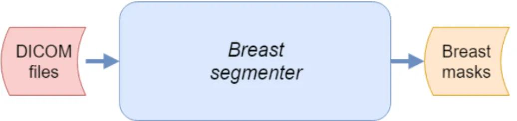
Afterwards, Chapter 3 describes the set of developed algorithms as a system where CT scans are viewed as inputs, and breast masks are viewed as the final output of the system. In each section is described the algorithms to process and segment the image, namely, how to and why segment the body, sternum and dorsi, and how the breast contours are detected using a shortest path algorithm. Finally, Chapter 4 presents the conclusion of the thesis, as well as some future work topics that are identified.

Chapter 2

Literature Review

In this chapter is done a literature review of the state of the art. In the first section, section 2.1, we will look at a brief review about the human body anatomy and some anatomical regions of interest about the breast. Afterwards, we review medical imaging technologies, section 2.2, and how medical images are stored in files (subsection 2.2.3). In the section 2.3 are described the main segmentation algorithms reviewed.

2.1

Thorax anatomy

The thoracic segment of the torso, also known as thorax, is shaped as an irregular cylinder. The thorax houses vital organs like the heart, the lungs, and great vessels. It also provides a means for the breathing process. Its musculoskeletal wall consists of vertebrae, ribs, muscles and the sternum, enclosing and protecting the thoracic cavity. The breasts are in the pectoral region on each side of the anterior thoracic wall (Figure 2.1) [1].

2.1.1 Breasts

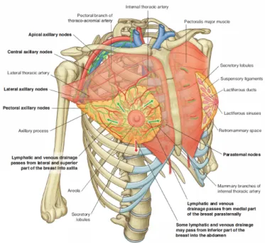
The breasts are located in the pectoral region, overlying the pectoralis major muscle. Al-though they vary in size, are normally positioned between the second and sixth ribs vertically, and between the sternum to as far as the latissimus dorsi muscle transversely (Figure 2.5) [1].

The breasts consist of mammary glands, associated skin, and connective tissues. Each gland extends around the lower margin of the pectoralis major muscle and enters the axilla, forming the axillary process of the breast. Mammary glands are a series of ducts and associated secretory lobules, converging onto the nipple, on the surface. The nipple is surrounded by a pigmented area of skin termed the areola (Figure 2.2) [1, 3].

6 Literature Review

Figure 2.1: Representation of the thorax anterior view. It also scheme the breasts, the pectoralis majorand the sternum. Image retrieved from [1].

Figure 2.2: Surface view of the breasts. Image retrieved from [2].

It is possible to see in Figure 2.3 that the breast is tear-shaped, where fat surrounds the mam-mary glands and extends throughout the structure that has no muscle tissue. This subcutaneous fat covers the network of ducts formed between the mammary glands and the nipple [1].

2.1.2 Chest muscles

The pectoral region contains three main muscles - the pectoralis major, pectoralis minor and subclavius muscles. These muscles form the anterior thoracic wall and the anterior wall of the axilla (Figure 2.4). The pectoralis major is the largest and most superficial, being directly under the breasts, only separated from it by loose connective tissue. It originates from the anterior surface

2.1 Thorax anatomy 7

Figure 2.3: Sagittal representation of the breast. Image retrieved from [3].

of the clavicle, the sternum, and related costal cartilages. Its functions are adduction, rotation and flexion of the humerus at the shoulder joint [1].

The pectoralis minor and subclavius underlie the pectoralis major. Both have the function of pulling the tip of the shoulder inferiorly. The small subclavius passes laterally from the anterior and medial part of the first rib to the inferior surface of the clavicle, while the pectoralis minor passes from the anterior surfaces of the third to the fifth rib to the scapula [1].

8 Literature Review

2.1.3 Latissimus dorsi

Latissimus dorsiis a superficial back muscle. It is triangular-shaped, large and flat.

Originates from the lower portion of the back and inserts into the humerus anteriorly, and as a result, has functions of extension, adduction, and rotation of the humerus [1].

Being a back muscle that inserts into the anterior portion of the humerus, its location defines the breast posterior portion, as seen in Figure 2.5.

Figure 2.5: Representation of the relation of the breast with adjoining structures. Image retrieved from [1].

2.2 Medical Imagining 9

2.1.4 Sternum

The sternum (represented on the center of the thorax in Figure 2.1) is an anterior medial bone that consists of the elements [1]:

1. The broad manubrium, superiorly positioned. Forms part of the bony framework of the neck and the thorax. The manubrium and the body join together at the sternal angle, where the junction forms a slight bend;

2. The flat narrow body of the sternum, longitudinally oriented. It has articulations with the ribs. The inferior end is attached to the xiphoid process;

3. The smallest part of the sternum is named xiphoid process, It is inferiorly positioned. The chest muscles originate from the sternum. Due to that, the sternum defines the breast anterior medial portion (Figure 2.5).

2.2

Medical Imagining

Medical imaging allows medical researchers and doctors to see anatomical structures inside the living body. It was German physicist Wilhelm Röntgen (1845–1923) that discovered the "X-ray" image, a "mysterious and invisible "X-ray" that passed through his flesh and left an outline of his bones on a screen coated with a metal compound, while experimenting with electrical cur-rent [26]. In 1895 he produced the first radio graphic exposure of his wife’s hand [1]. This discovery rewarded him with the Nobel Prize for physics [26].

2.2.1 Anatomical planes

For describing the location of structures relative to the body or other structures, there are three major pairs of terms that are used [1]:

• Anterior and posterior relate the structure with the front and the back of the body. For example, the sternum is anterior the the latissimus dorsi muscle, with the former being posterior to the latter;

• Medial and lateral describe the relation between structures and the middle sagittal plane of the body. For example, the nose is medial to the eyes, and the thumb is lateral to the little finger;

• Superior and inferior describe the location of structures regarding the vertical axis of the body.

10 Literature Review

Assuming a standard position, there is three major groups of planes that pass through the body.

Figure 2.6: Anatomical planes and reference. Image retrieved from [1].

Those are:

• The axial planes, that divide the body into superior and inferior parts;

• The sagittal planes, vertically oriented, which divide the body into left and right;

• The coronal planes, also vertically oriented, but instead divide the body into anterior and posterior parts.

Figure 2.6 shows the three major planes sectioning the body, while also exemplify the posi-tional reference terminology used.

2.2 Medical Imagining 11

2.2.2 Computed Tomography

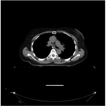
Also called Computerized Axial Tomography, CT was invented by Sir Godfrey Hounsfield, Nobel Prize winner in Medicine in 1979 [1]. In this technique, the patient lies in a motorized platform while a CT scanner (Figure 2.7) obtains X-ray images in the axial plane by rotating 360 degrees around the patient. A computer combine these forming a axial view of the area, or "slice" (Figure 2.8) [26].

Figure 2.7: CT scanner. Image retrieved from [1].

According to [1], air attenuates X-ray the least, bone the most, and fat attenuates more than air but less than water. Due to this, things on the image will be whiter (higher pixel intensity) the less they attenuate X-ray, and darker the more they absorb.

The images are viewed such that the observer looks from below and upward toward the head. By implication the right side of the patient is the left side of the image, and the uppermost border is anterior.

2.2.3 DICOM files

Digital Imaging and Communications in Medicine (DICOM) is a protocol for storage and transmission of medical information. It was developed by the American College of Radiology (ACR) and National Electrical Manufacturers Association (NEMA). After the development of the

12 Literature Review

Figure 2.8: Ct slice example. Axial view. Imaging data provided by Fundação Champalimaud.

CT scanner and other imaging devices, it was very difficult for anyone other than the manufacturers of the devices to decode the images generated. DICOM was released in 1993, based on previous standards developed by ACR/NEMA [27].

One DICOM file has the information contained into data objects, which consists of a number of attributes, for example, patient data, machine information and other detailed information. This way, the image can never be separated from the patient data, with the image (Figure 2.8) itself being a data object of the DICOM file [27].

2.3

Image Segmentation Algorithms

A image is, in a broad sense, a representation of an object. Image segmentation tries to partition an image according to some meaning [28] or common property [20]. Segmentation of medical images aims to locate anatomic structures [17] and tissue types [29]. According to [30], image segmentation is one of the most critical tasks of image analysis.

In a study by [17], the author identifies segmentation algorithms used in images meant for RT planning. He classifies the algorithms into methods that are not using prior-knowledge, and

2.3 Image Segmentation Algorithms 13

methods powered by prior-knowledge, as well as hybrid methods, that are composed by methods of both groups.

Traditional autosegmentation methods are based in image content like pixel intensity and gradient. Among them, methods such as thresholding, graph cuts and watershed segmentation have been used for RT planning [17].

2.3.1 Thresholding

Thresholding are some of the simplest segmentation methods. It transforms an image into a binary, dividing the image into two segments [21]. It can be defined as [28]:

IT(x, y) =

(

1, if I(x, y) > T

0, if I(x, y) ≤ T (2.1)

T can be a constant (global thresholding) applied to the whole image or a function of x and y, in that case the method is named adaptive thresholding [21]. Its value can be found by analysing the image pixel intensity histogram, and choosing the minimum value between peaks (optimum with bi-modal histograms). This is known as the Otsu method [31].

According to [30], one of it main limitations is that it does not take into account spatial characteristics of an image.

2.3.2 Clustering algorithms

The goal of this family of algorithms is to segment the image in a set of disjoint groups, or clusters. Different properties can define a cluster. These algorithms are common when the number of classes is known beforehand.

K-means clustering is a type of clustering algorithms, where each pixel belongs to one of k groups after each of n observations, in which the observation belongs to the cluster with the nearest mean. According to [28], this is an NP-hard problem, but some efficient heuristic algorithms can converge to a local optimum.

Adaptions of this algorithm exist, e.g., fuzzy C-means for fuzzy clustering, where each pixel can belong to more than one cluster [28].

2.3.3 Edge detection

An edge is a high-intensity gradient between neighbors pixels in an image, i.e., an edge is a group of pixels that present a rapid transition in intensity, when compared to their neighbors [28].

14 Literature Review

Rebelo, J. [28] reviewed active contour models algorithm, which tries to segment images along the edges keeping a smooth segmentation border. The algorithm, also known as snakes, describes parametrically defined contours (snake) that move in a image as v(s) = [x(s), y(s)], where x(s) and y(s) are the coordinates of the contour for part s. These contours move while trying to minimize their energy composed of an internal and external component. The internal energy is controlled by the deformations made to the snake, while the external energy consists of a combination of constraints introduced by the user and forces of the image [28].

Detecting edges can also be viewed as a problem of finding the minimum cost path in a directed weighted graph [32].

2.3.4 Region Based Algorithms

Region-based segmentation algorithms build disjoint regions by merging neighbor pixels with similar characteristics together, according to predefined criteria [31, 28, 30]. There are two main types of these methods: region growing and region splitting and merging.

2.3.4.1 Region growing

Starting from a group of pre-established seed pixels, the region is iteratively increased, ap-pending similar neighboring pixels [28]. The seed pixels belong to the structure of interest [31]. This procedure ends when no more pixels can be added to the given region, i.e., some stopping criterion is met [28]. It is possible that at the end of the iterative process, some pixels are not labeled [31]. According to [31] this method is similar to breadth-first search.

According to [20] region growing is especially useful when the structures are separated spa-tially. [31] the results of this algorithm depend strongly on the selection of the homogeneity criterion. Another problem identified by the same author is different starting points not growing into identical regions.

2.3.4.2 Region Splitting and Merging

The main difference between this and the previous method is that in region splitting and merging there is not a choice of seed points, but the image is iteratively divided into a set of unconnected regions and then when no further splitting is possible, those regions are merged [28] according to the previous criterion.

2.3 Image Segmentation Algorithms 15

2.3.5 Watershed

Watershed is a region-based algorithm that uses image morphology. It sees the image as a topographic relief, where the grey level is seen as the altitude in the relief [31].

“Water” flows from the points where the altitude, and therefore the pixel intensity, is lower. Then, the watersheds in the topographic landscape will be flooded at a constant rate, and when are about to merge, a watershed line is created. This continues until all the landscape is flooded, i.e., until the pixel with maximum intensity [20]. The watershed lines mark segmentation borders [28]. This algorithm is deemed to be a powerful tool for segmentation [31], being used in medical imaging segmentation in RT planning [17]. However, it tends to over-segmentation when the images are noisy or the desired structures have low Signal-to-Noise Ratio (SNR) [31].

2.3.6 Atlas based segmentation

In atlas based segmentation prior knowledge is used. It is applied using a reference image, an atlas, in which structures are already segmented. The goal is to find the optimal transformation between the atlas image and the test image.

The atlas has a crucial role in the segmentation. The morphology of the ROI should be similar in atlas and test images to establish valid correspondences. The usage of a general anatomy patient atlas improve the segmentation results [17].

According to [4], in a study of the performance of an atlas-based autosegmentation software for delineation of target volumes for RT of breast and anorectal cancer, this automatic segmen-tation method show promise to reduce contouring time and variability, but still have to undergo further improvement.

To quantify results, Anders et al. [4] defined three parameters, the Dice Similarity Coefficient (DSC), the logit transformation of the DSC and percent overlap.

DSC is used to evaluate the similarity of manually and automatically segmented structures and is defined as

DSC(A, B) = A_A+B∩ B

2

(2.2) where A and B refer to the manually segmented and the auto-segmented structures, respectively. The need for the logit transformation arises from the fact that DSC results in values between 0 and 1, and there is a tendency to often approach 1.

Satisfactory results were retrieved, which are presented in table 2.1. Anders et al. [4] point out that it seems that the decisive factor for the results of auto-segmentation is the shape of the breast and not so much the breast volume itself – that being suggested by the results of the medium

16 Literature Review

atlas over all the nine patients. Simultaneous truth and performance level evaluation (STAPLE) algorithm, which employs a strategy of multi-atlas fusion for autosegmentation to improve the accuracy of the segmentation process, further improves these results by integrating the three atlases covering the whole spectrum of breast geometries.

CTV Atllas/patient DSC Logit(DSC) PO Small/1-2 0.86 1.82 75.50% Small/1-9 0.86 1.83 75.96% Medium/3-6 0.89 2.12 80.75% Medium/1-9 0.90 2.19 81.44% Large/7-9 0.91 2.36 82.30% Large/1-9 0.87 1.96 76.89% STAPLE/1-9 0.91 2.27 82.89%

Table 2.1: Results from Anders et al.. Retrieved and adapted from [4].

2.3.7 Statistical models

The use of statistical shape and appearance models typically provide closed and anatomically correct surfaces [17]. The final segmentation result is restricted to plausible shapes described by a model. It undergoes a training phase were the model learns from an set of images with correct delineation of structures. The main disadvantage of this methods is its low flexibility, due to being limited by the training set size.

2.4

Conclusion

RT planning needs accurate delineations of anatomical relevant structures for maximum ef-ficiency of treatment. Automatic image segmentation can decrease contouring time consumption, and reduce variability, but due to the variability of the breasts size and shape, methods based on prior knowledge and/or shape can still be aided by methods based on pixel information.

Despite the trend of knowledge based algorithms, breast segmentation lacks of an established ground truth. Even using state of the art algorithms like STAPLE, the breast shape and volume difference to the reference atlas used has implications on the segmentation results. Also due to this variability, statistical models need a large training data set to be able to cover a broad spectrum of different breast geometries.

Due to CT scan nature, where different types of tissues show different pixel intensity, some relevant information can be obtained. While the breast is mostly composed by fat, the adjacent anatomical structures are mainly composed of muscle (chest wall) and bone (sternum). Due to

2.4 Conclusion 17

this, and as on CT images, breast tissue will have pixel intensities lower than muscle tissue, edge based detection algorithms are natural candidates to obtain a contour of the breast.

Edge detection by finding the minimum cost path in a directed weighted graph has advantages over methods such as watershed, whom tends to provide a closed contour but over-segment images, or snakes algorithm that cannot handle contour splitting or merging [33].

Thresholding algorithms have a part on the processing stage of the segmentation workflow, enabling to adjust, focus and obtain different ROI, e.g., allowing to easily obtain a bone structure view from images like Figure 2.8.

Chapter 3

Breast Segmentation

This chapter presents the main design choices for the developed algorithms, problems that arose from the implementation and possible improvements. For breast contour and tumor bed detection algorithms validation, data provided by Fundação Champalimaud is used, with the first algorithm being validated within six sets of images, and

3.1

System requirements

The aim of this work is to develop a system capable of receiving as an input a series of DICOM data elements that represent a CT study of the chest of a patient, and outputs masks corresponding to the breast and tumor bed ROI. Given the nature of the problem, the system is realized as a Python program.

Figure 3.1: System schematic.

3.1.1 Image handling

Medical image is encoded in DICOM format, as seen in section 2.2.3. Pydicom Python module was used to extract, view and manipulate image pixel data, which provides a easy to use way of reading DICOM data structures into Python code. This also allowed to develop a simple

20 Breast Segmentation

interface to use open-source library OpenCV bindings for Python, since both modules rely on the NumPy package for scientific computing for containing image data.

It was developed a package that allows to, given a set of DICOM files, read and view a 3D representation of the data. It also allows to retrieve the axial, sagittal and coronal 2D views. It contains a set of methods to process the images and obtain masks for various anatomical structures, like the sternum, breast and tumor bed.

All image processing is done by using OpenCV methods.

3.1.2 Utility functions

To help with the manipulation of the images, it was developed some utility functions: • Setting the window of visualization of the CT image, given the Window Width and Window

Center DICOM attributes;

• Obtaining axial, sagittal and coronal views from the 3D volume of images;

• Image normalization and conversion to 8 bits unsigned (DICOM uses 16bit unsigned en-coding);

• Cartesian to polar and vice-versa image transformation.

• Mass center computation, by using OpenCV moments function, which compute polygons image moments up to the third order.

3.1.3 System Breakdown Structure

To obtain the breasts and tumor masks, given the CT scan images, the system must be able to detect where is the breast origin and termination point. As seen in section 2.1, breast tissue lies over the thoracic wall, originating from the sternum in the anterior medial portion, and extends to the latissimus dorsi muscle in the posterior portion. For that reason, the system must detect those anatomical structures, that will work as seed points for the minimum cost path algorithm to work on.

Nevertheless, the system should also be capable of extracting pixel information about the anatomical structures. As different types of tissues have different pixel intensity values according to X-ray absorption rate, as seen in section 2.2, a coarse categorization of those pixels provide valuable information, e.g., it allows to threshold the image to obtain only pixels that can be seen as bone tissue or a X-ray absorption rate equivalent. As such, a coarse body segmentation is also an important part of the system.

3.2 Body Information 21

Figure 3.2: System Breakdown Structure.

3.2

Body Information

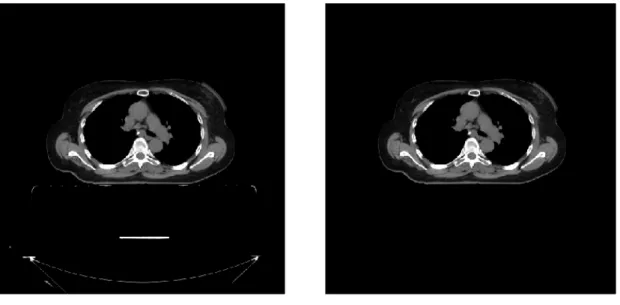
As seen in section 3.1.3, one requirement is to segment the body in the CT scan, given that it provide information about the patient center of mass together with the segmentation masks. These masks allows to remove artifacts from the CT scanner, such as the table contours, as can be seen in Figure 3.3.

(a) Table artifacts on image. (b) Image clear of artifacts.

Figure 3.3: Effect of clearing artifacts from the image in axial view.

22 Breast Segmentation

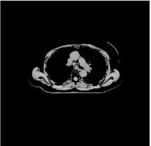
multi-level Otsu algorithm to retrieve two optimal pixel values from the image histogram. I.e., we assume that there is three main classes of pixels, where very low intensity pixels represent air, fat and other tissues that have small X-ray attenuation coefficients, very high intensity pixels represent bone tissue and other structures with high X-ray attenuation, and between those two values are represented soft tissues like muscles, e.g.. In Figure 3.4, those thresholds are applied to Figure 3.3b, resulting in different views of the body.

(a) Soft tissue view of the body.

(b) Bone structures view of the body.

Figure 3.4: Thresholding the image with multi level Otsu values result in obtaining different views of the body.

This algorithm assumes that the body contour is the contour with the highest contour area in the image, as highlighted in Figure 3.5, where the drawn red contour represents the contour with

3.2 Body Information 23

highest area and the blue contours are all the other external contours detected. It also uses previous masks information for detecting if smaller contours are still connected with the body, given that the patient scan position is in dorsal recumbency (i.e., face-up on the table) with their arms raised next to the head, as seen in the mask represented on Figure 3.6.

Figure 3.5: Highest area contour represented upon the respective slice.

(a) Axial slice of the superior body portion, where the arms are raised next to the head.

(b) Body mask outputted by the body segmenta-tion algorithm.

Figure 3.6: Mask retrieved from body segmentation algorithm in superior slices, properly detect-ing the arms raised next to the head.

24 Breast Segmentation

The algorithm is presented in Algorithm 1: Algorithm 1: Body segmentation algorithm.

Input: 3D set of CT images

Output: 3D body masks, body mass center pixel and thresholds

# Initialization

Create structure for masks with same shape as 3D representation Obtain axial view

Mass center vector = [] Thresholds vector = []

# Detection loop

while n < number slices do Create binary representation Obtain detected contours

Sort contours by area, highest first foreach cnt in Contours do

if Overlay with previous masks then cnt is body

else

continue

Mass center vector[n] calculation using contour moments Image artifacts removal

Multi-level Otsu algorithm to compute thresholds[n] MC = mean of all the 2D slice mass centers

Thresholds = mean of all the thresholds

3.2.1 Center of Mass

The center of mass is computed by retrieving the body contour moments and obtaining the contour centroid pixel position:

Cx=

m10

m₀₀; Cy= m01

m₀₀ (3.1)

Image moments are weighted average of the image pixel intensities. They are computed according: Mpq= Z ∞ −∞ Z ∞ −∞ xp· yq_{· I(x, y) · dx · dy (3.2)}

3.3 Segmentation of the Sternum bone 25

3.2.2 Multi-level optimum threshold values

Due the nature of the CT scan, where different tissues with different radio-density appear with varying gray scale intensity, it was implemented a method to retrieve two optimal thresholds values. This allows to bin pixels into three groups such as air or fat tissue, soft tissues like muscle and bone. The implemented algorithm was described in Ref. [34].

The correspondence coarsely can be done like represented in Figure 3.7, where we can see an histogram of a slice, after removing artefacts caused by the scanner. In it, the red and blue vertical bars mark the obtained threshold values.

Figure 3.7: Histogram with two optimum thresholds.

3.3

Segmentation of the Sternum bone

The sternum is the most medial bone in the anterior portion of the body from which originate the chest muscles, forming the thoracic wall and as such, it marks the breast anterior medial limit. For that reason, the implemented breast contour detection algorithm relies on being feed with a set of masks that segment the sternum.

As such, a sternum segmentation algorithm was developed and implemented (Algorithm 2). Since the CT scan is done to the thoracic portion of the body, it is assumed that the axial slice in the izcoordinate such as iz= max(z)/2 always contains a view of the sternum (Figure 3.8a), and

that it is the most anterior contour after obtaining a thresholded image to represent only the bone structures in the CT image, as in Figure 3.8c. I.e., contours are ordered according to the distance

26 Breast Segmentation

between them and the point given by the cmx and the y of the body bounding box, identified in

Figure 3.8b.

(a) Axial slice in the middle of the z axis of the 3D volume of im-ages. The algorithm assumes that the sternum is always represented is this slice.

(b) Thresholded view of the bone structures, and representation of the point from which distance to contours is measured.

(c) Obtained contour represented over the image.

Figure 3.8: First step of the sternum detection algorithm.

This assumption provides a 3D set of seed voxels, allowing to employ a region growing algorithm to obtain the full segmentation of the structure, in two steps. First, using a sagittal view, allowing to spread seed voxels along the z axis, as seen in Figure 3.9, and finally looping through all the axial slices. This is done by thresholding the image to obtain a representation of the bones, and then checking which contours overlap the seed points.

The algorithm outputs the 3D volume of the segmented structure and a number of computed parameters that improve the workflow of the developed algorithms, e.g., the index of the z axis of the first and last detection of the sternum, and a projection of the sternum centroid in the yx plane.

(a) Sagittal slice of the sternum center of mass. (b) Contour which overlap the seed points ob-tained in the previous step.

3.4 Dorsi Points 27

Algorithm 2: Sternum segmentation algorithm.

Input: 3D images, Body 3D masks, Body center of mass, Threshold for obtaining bone structure view

Output: 3D sternum masks, sternum start slice, sternum end slice and mass center point

# Initialization

Create structure for masks with same shape as 3D representation Obtain axial view

Obtain sagittal view

# Obtaining seed points

Obtain mid-slice in axial view (img = axial_view[nr_slices/2])

Threshold that image using threshold value related with bone structures Define limit_point = body_mcx, body_contoury

Obtain contours and sort them by distance to limit_point, lowest distance first Save mask obtained from the contour in sternum 3D structure

Obtain mass center for that slice

img= sagittal_view[sternum_mass_center_x]

Threshold that image using threshold value related with bone structures

Given the seed points obtained by the axial detection, obtain the contour which the points lie within

Save mask on 3D structure

Find slices where sternum 3D structure is non-zero in z axis

# Looping through axial slices

for axial slice in (sternum_start, start_end) do

Given the seed points obtained by the previous detections, obtain which contour the points lie within

end

Compute sternum structure centroid

3.4

Dorsi Points

Dorsi detection allows the algorithm to set a breast contour termination, since the breast contour detection algorithm searches for the minimum cost path between two points.

It was developed an algorithm (Algorithm 3) for detection of an estimation of the location of the latissimus dorsi, taken from a user-defined number of slices that search in axial slices close to the medial z coordinate of the sternum, i.e., the algorithm detects the dorsi in half of the user-defined number of slices above the starting slice, and other half below.

28 Breast Segmentation

This design choice arose from the fact that the latissimus dorsi shape variation between slices is considerable, but in the mentioned before ones the muscle has a peaked shape in the axial view (Figure 3.10). This allows to search in a soft tissues (muscles) only view where the muscle contour tangent is constant, being that pixel taken as the dorsi point. In the developed algorithm, a secant function is used, since if the slope of the secant approaches a limit value, then that limit defines the slope of the tangent line at that given point.

The algorithm outputs the average of all detections, providing a projection in the yx plane for the latissimus dorsi location in the slice.

Figure 3.10: Axial slice in the medial z coordinate of the sternum, where the latissimus dorsi muscle has a peaked shape.

3.5 Breast 29

Algorithm 3: Dorsi segmentation algorithm.

Input: Number of slices to scan, 3D images volume, 3D Body masks, Sternum medial z coordinate, Thresholds

Output: Right and left dorsi pixels estimation

# Initialization

Obtain axial view n= 0

up_down = False

# Looping through axial slices

while n < n_slices_dorsi do

idx= mid_sternum + n + (−2 · n · up_down) img= axial_view[idx]

Obtain muscle view and muscle contour from img Obtain gradient image from img

From gradient image indexes, find minimum and maximum x coordinate of the muscle contour

Find corresponding y coordinates for each ix

The contour must start from the previous computed edge points and grow in the y coordinatesa

secant_vector_le f t = secant(le f t_sorted_contour) secant_vector_right = secant(right_sorted_contour)

dorsi_le f t = le f t_sorted_contour[argminb_{(secant_vector_le f t)]}

dorsi_right = right_sorted_contour[argmin(secant_vector_right)] up_down =!up_down

n+ = 1 end

Dorsipixel estimation is the mean of the points where the computed secant value is minimal.

a_{Contour ordering to obtain a clockwise ordered contour starting at previous edge point for the left side of the image.}

OpenCV detects contours and creates a list of points ordered by lowest to highest y coordinate, ordering the x coordinate counter-clockwise.

b_{argmin is the index of the minimum in the vector.}

3.5

Breast

The breast is composed by subcutaneous fat, that appears as lower intensity pixels in CT images than the adjoining structures, usually. As seen in section 2.1, the sternum bone and the latissimus dorsi define the anterior and posterior limits of the breast, respectively. Given that, breast segmentation can be seen as an edge detection problem or a minimum cost path in a graph between those points.

30 Breast Segmentation

In the developed algorithm (Algorithm 4), breast contours are detected using an algorithm to detect the minimum cost path between two points. Margin points are computed from the sternum centroid and the estimated point for the dorsi muscle. For the external contour, the point in the body contour closer (in euclidean distance) to the sternum centroid and the dorsi pixel is the chosen. For the internal contour, the dorsi point is itself the margin point, while in the sternum it is chosen the point on its contour closer to its center of mass.

This algorithm segments both breasts in the extension of the sternum bone, along the z axis. While for the external contour detection there is no processing done to the image (Figure 3.3), for the internal contour the image is thresholded to retrieve a view of muscle tissue (Figure 3.4a). This allow the performance of the algorithm to increase, since while searching for the inner contour created by the chest wall, very high and very low intensity pixels will not affect the results.

The algorithm loops through all the axial slices where the sternum masks are present. Con-tours are taken one at a time, starting with the computation of the margin points, followed by the transformation in a polar image between the given angle. The polar image is then inverted and its gradient is obtained, which is fed to the minimum cost path algorithm, that outputs the polar contour. Finally, for each breast the contours are concatenated and the axial mask is drawn.

The output of this developed algorithm is two 3D volumes of masks, one for the right and another for the left breast.

Algorithm 4: Breasts segmentation algorithm

Input: 3D images volume, 3D Body masks, 3D Sternum masks, Dorsi pixel index, Thresholds, Angle resolution

Output: Right and left 3D breasts masks.

# Initialization

Initialization of both 3D structures

Definition of the function object to obtain minimum path algorithm margin points

# Looping through axial slices between sternum z coordinates

for min sternumz< n <max sternumzdo

internal_image = Threshold image to obtain a soft-tissue only view

# For each contour

Create polar image from img

Compute polar coordinates of the margin points Invert image

Obtain gradient of the image

Apply minimum cost path algorithm

# # #

Create mask from detected contours end

3.5 Breast 31

3.5.1 Minimum cost path algorithm

A minimum cost path detection algorithm is a graph cost minimization algorithm. Treating the image as a graph, given a point that is enclosed by a path and transforming the image into polar coordinates, that closed path transforms into the shortest path between opposite margins, given that the wanted point is the origin [33]. The implemented algorithm is presented in [35].

The implemented version is fed by the gradient of an image, and applies a cost function over it. After that, it does the computation of the cost matrix, and finally iterates over it to find the minimum cost path between the margins. Search type is a parameter between point to point, margin to margin or any combination between them.

The parameters used in the weight function

f(g) = fl+ ( fh− fl) ∗

exp(β · (255 − g)) − 1 exp(β · 255) − 1 [35]

were fl= 2, fh= 128 and β = 0.25, where g is the derivative of the image. For 8-neighbour pixels

the weight was set to√2 times that value.

Figure 3.12 shows the result of the algorithm applied to the external contour of the breast. As the image is in polar coordinates, Figure 3.12a presents the same contour, but plotted in Cartesian coordinates in the full picture.

(a) Polar coordinates. (b) Cartesian coordinates

32 Breast Segmentation

Table 3.1: Breast external contour segmentation results. All the values are expressed in pixel distance. Contour to Ground Truth Ground Truth to Contour Euclidean Distance Hausdorff Distance Euclidean Distance Hausdorff Distance Patient Mean SD Mean SD Mean SD Mean SD

1 Left Breast 1.90 0.59 10.66 7.67 1.69 0.63 8.27 5.78 2 Left Breast 1.55 1.10 13.1 10.0 0.97 0.50 4.49 2.64 3 Right Breast 1.51 0.15 4.69 2.87 1.49 0.22 5.38 3.85 4 Right Breast 4.69 4.36 42.28 20.02 1.25 0.65 9.08 7.55 5 Left Breast 2.26 1.85 21.61 11.54 1.15 0.83 5.94 6.68 6 Left Breast 2.83 2.40 26.60 12.63 1.38 1.95 3.91 4.36 Average 2.46 1.74 19.82 10.79 1.32 0.79 6.17 6.17 3.5.2 Results

To validate the obtained contours, they were compared to contours provided by experts that will be considered as ground truth. Comparison metric was chosen to be the Hausdorff distance and the average distance between the detected contour and ground truth, and vice-versa. This metric was chosen because it represents the worst case scenario, as stated in [36]. Results for the external contour detection are presented in Table 3.1 and results for the internal contour detection are presented in Table 3.2.

The Hausdorff distance between two sets of points is defined as

h(A, B) = max

a∈A minb∈B k a − b k [36]

where k · k is the Euclidean distance.

Despite pixel spacing being different among the test subjects, it presents an average ratio of 1 pixel to 1mm, with σ = 0.02. This results show that the algorithm is capable of detect con-tours close to what is taken as ground truth, having low average and Hausdorff distances between contours.

One of the main advantages of the algorithm when compared with other methods is that it does not depend directly of a previous set of images to segment the breasts, and as such, it is able to perform in the full spectrum of body and breast shapes and sizes.

3.5 Breast 33

Table 3.2: Breast internal contour segmentation results. All the values are expressed in pixel distance. Contour to Ground Truth Ground Truth to Contour Euclidean Distance Hausdorff Distance Euclidean Distance Hausdorff Distance Patient Mean SD Mean SD Mean SD Mean SD

1 Left Breast 1.29 0.54 8.96 3.64 1.18 0.73 8.14 5.13 2 Left Breast 2.51 2.88 10.86 8.90 2.00 2.17 9.24 7.05 3 Right Breast 1.41 0.94 9.13 4.71 1.05 0.63 6.83 3.94 4 Right Breast 6.17 4.36 22.67 11.63 4.41 3.86 16.30 9.75 5 Left Breast 2.85 1.86 14.29 4.27 2.60 2,03 12.4 7.05 6 Left Breast 3.29 1.28 18.16 8.39 2.43 1.27 10.24 3.90 Average 2.92 1.97 14.01 6.92 2.28 1.78 10.34 6.14

Despite the positive results, it is shown that the algorithm performance is completely degraded by errors in the choice of the margin points for the minimum path algorithm. In the example given by Patient 4, due an error in the dorsi point computation, the point taken as the external point for the latissimus dorsi muscle is more posterior than the ground truth posterior origin of the breast 3.13.

(a) Patient 4 slice. (b) Breast mask drawn from the contours obtained by the mini-mum cost path algorithm.

(c) Overlay of the body with the breast mask, where part of the dorsi muscle is visible.

Figure 3.13: Implications of an error at computing margin points.

Due to the algorithm assumption that fat has a lower pixel intensity value than muscle tissue, the algorithm has low performance where this does not hold true. Some breast tissue can have higher pixel intensity than what is taken as the muscle tissue threshold. In that case, results are not

34 Breast Segmentation

coherent, i.e., the detected contour may not be only muscle tissue, and as such it does not define the chest wall and the inner breast contour, as seen in Figure 3.14 and Figure 3.15. The previous cause of error is closely related to this, since dorsi points are computed under the assumption that the latissimus dorsi is the wider contour within the given pixel intensity range and when it does not hold truth, the results present a large margin of error.

Figure 3.14: Higher pixel intensity in breast tissue.

(a) Higher pixel intensity in breast tissue.

(b) Breast mask drawn from the contours obtained by the mini-mum cost path algorithm.

(c) Overlay of the body with the breast mask, where breast fat was taken as chest wall.

Figure 3.15: Implications of high pixel intensity on breast fat.

Nevertheless, the fact that the algorithm is implemented in a highly dynamic programming language, with a strong emphasis in modularity, allow that the detection of the dorsi points and the algorithm to bin the pixel intensity into categories to be improved in the future.

3.6 Tumor detection 35

3.6

Tumor detection

Since RT planning is done post surgery for removal of the tumor, what is in fact segmented as the tumor bed are markers placed by the surgeon. Those markers have the peculiarity of being X-ray attenuators, and so they are translated into the image with a high pixel intensity. For that reason, the implemented algorithm is fed by the 3D volume of breast masks, and, in the axial view, thresholds the breast area.

This algorithm has an associated error due to the fact that that patients are lied with their arms raised, and if they have a tumor bed in the axillary process above the min sternumzcoordinate,

it will not be properly segmented. Also, this algorithm does not take into account tumor beds that spread into the chest wall, given that it only searches within the breast mask area. Future improvements could add support to check within the chest wall, provided a proper segmentation of that structure.

Region growing algorithms are also not capable of segment properly in those conditions, given the fact that the markers do not necessarily make a close region.

Algorithm 5: Tumor bed segmentation algorithm.

Input: 3D images volume, 3D Breast masks, Thresholds Output: 3D tumor mask

# Initialization

Obtain axial view

# Looping through axial slices

for n in nr_slices do Obtain image

Using breast mask as ROI, threshold the image Thresholded image is the tumor mask

end

3.6.1 Results

Given that the tumor bed segmentation is done based on the 3D contents of the images volume and the breasts masks, the metric chosen to evaluate the segmentation was the computation of the 3D tumor masks centroid and comparison with some known ground truth, through the euclidean distance.

For validation, four sets of images provided by Fundação Champalimaud were used. Ground truth manual delineations of the breast were fed into the developed tumor bed detection algorithm, and then the resulting 3D volume of binary masks was used into the metric calculation.

36 Breast Segmentation

Table 3.3: Results for the tumor segmentation validation. Distance in pixels.

Patient Euclidean Distance 1 1.07 2 2.75 3 2.28 4 5.06 Average 2.79 Standard Deviation 1.45

This results show that simple thresholding algorithms combined with the knowledge of how different tissues have different gray-scale pixel intensity in CT scans is a powerful tool to provide a starting point to radiologists in the process of delineating structures and lesions for improving radiotherapy. Plus, the described algorithm has an inherent error due to its limitations, that can be further improved.

Despite this, this metric is sensible to any false-positive detection in the breast segmentation, e.g., if any CT artefact is delineated together with breast tissue, as it affects the detection centroid.

3.7

Conclusion

With the goal of providing a breast and tumor segmentation, it was developed a set of algo-rithms that fulfill that objective, and also segment some adjoining structures. This chapter pre-sented a detailed description of the makings, the inputs and outputs of each of those algorithms, as well as validation results for the breasts and tumor bed detection algorithms.

To segment the breast, we have proposed a algorithm that detect the contours of this anatom-ical structure, by minimization of the cost of the contours within the image, when interpreting the image as a graph. Despite the trend into machine learning and knowledge based algorithms, those algorithms have the need for a large training data, to cover the spectrum of breast shapes and sizes. The proposed algorithm overcomes that limitation by relying on the pixel intensity information.

For the tumor bed, the proposed algorithm focus on the ROI created by the breast tissue, given by the breast mask fed into the algorithm. With that information, it thresholds the ROI to find the tumor markers. It main limitations are that it is not able to fully segment the tumor bed on the axillary process and on the chest wall, and it is prone to error from the breast segmentation.

Chapter 4

Conclusions

Breast cancer is one of the most common malignancies, and also one of the most deadly diseases mankind is facing today. Despite treatment plans for early-stage breast cancer allow for survivability rates to increase, the dynamic nature of the disease, as well the time burden of the tasks involved in the treatment planning stage urge for tools that are able to improve the workflow of the treatment.

Despite the existence of new methods for automatic segmentation of the breast in CT scans, that use knowledge through learning, methods that rely on pixel information can improve the outcome of the final segmentation, since the human body in general, and the breast specifically, presents great variability in the shape and size of it anatomical structures. That variability requires that knowledge based methods, e.g., atlas based segmentation, to rely on large training data, that is not possible.

The main goal of this work was to develop and implement an algorithm capable of auto-matically detect and segment anatomical structures to improve the workflow of the RT planning stage, post breast conservative surgery for removal of a tumor. As such, this work focused on segment the breast and the tumor bed, such as the sternum and the latissimus dorsi muscle, whose segmentation masks fed the breast detection algorithm.

To segment the breast, given the previous segmentation of the enclosing anatomical struc-tures, we chose to see the problem as a cost minimization problem, in order to find the desired contours. As such, implementing a minimum cost path algorithm, segmentation results presented in Table 3.1 and Table 3.2 show that between the algorithm detection and a delineation from an expert, the contour distance is in the order of millimeters. Despite those positive results, Hausdorff distance on some patients is in the order of centimeters. It is due to the assumptions that we did designing the algorithm, e.g., that between the pixel intensity of fat tissue and muscle tissue there is an optimum threshold level, that does not verify to all patients.

38 Conclusions

As these algorithms are to work in CT images taken after breast conservative surgery, where the tumor has been removed, and the tumor bed is marked by the surgeon, a first take on a tumor bed segmentation algorithm was to search for the highest intensity pixels within the breast tissue. This provide a starting point to the radiologist, allowing to relieving the burden of fully manual delineation, but does not provide a complete segmentation of the tumor bed, since it does not search for the tumor in the chest wall, and it may not search for it in the full extension of the axillary process. Measuring the distance between center of mass of the tumor bed detection, it shows that as seen in the results at Table 3.3, average distance between center of mass of the tumor detection and the ground truth is in the order of millimeters.

4.1

Future Work

Analysing the contributions made by this work, it is of the outermost importance to validate results against different data.

The developed algorithms were designed to retrieve useful information from the pixel data, but were developed taking into account external data input, i.e., they are modular. For instance, breast detection algorithm does not rely on our sternum detection algorithm, as it only needs a volume of 3D sternum masks of the same size as the remaining volumes. This create a window of opportunity to develop new methods to aid the detection done by the algorithm, further improving the obtained results, e.g., estimations the margin points for the detection of the breasts contours or methods to obtain different views of the image, within the scope of the DICOM Window Center and Window Width attributes, for instance.

Regarding the tumor detection algorithm, two main topics should be addressed in the future, namely the ability to segment the tumor within the chest wall and the ability to fully segment the axillary process portion of the breast.

Other metrics could had been chosen for results validation, e.g., DSC or percent overlap [4]. The mentioned metrics and the euclidean distance measure the approximation between the de-tected contour and some ground truth. But according to Gooding et. al. [37], these measurements may not reflect clinical adequacy. Further study about the relation between the presented error and real dosage difference is a step forward into providing insight about the quality of automatic segmentation methods.

References

[1] Richard L Drake, Wayne Vogl, and Adam W M Mitchell. Gray’s anatomy for students. Philadelphia: Elsevier/Churchill Livingstone, 2005.

[2] Ralf Roletschek and Sansbrassiere. Breast, 2005. URL: https://commons. wikimedia.org/w/index.php?curid=314112.

[3] Ikram E Khuda. A comprehensive review on design and development of human breast phan-toms for ultra-wide band breast cancer imaging systems. Engineering Journal, 21(3):183– 206, 2017.

[4] Lisanne C Anders, Florian Stieler, Kerstin Siebenlist, Jörg Schäfer, Frank Lohr, and Fred-erik Wenz. Performance of an atlas-based autosegmentation software for delineation of tar-get volumes for radiotherapy of breast and anorectal cancer. Radiotherapy and Oncology, 102(1):68–73, 2012. doi:10.1016/j.radonc.2011.08.043.

[5] National Cancer Institute. Radiation therapy for cancer, 2019. URL: https://www. cancer.gov/about-cancer/treatment/types/radiation-therapy.

[6] National Cancer Institute. What is cancer?, 2015. URL:https://www.cancer.gov/ about-cancer/understanding/what-is-cancer.

[7] World Health Organization. Cancer, 2018. URL:https://www.who.int/news-room/ fact-sheets/detail/cancer.

[8] Freddie Bray, Jacques Ferlay, Isabelle Soerjomataram, Rebecca L Siegel, Lindsey A Torre, and Ahmedin Jemal. Global cancer statistics 2018: Globocan estimates of incidence and mortality worldwide for 36 cancers in 185 countries. CA: a cancer journal for clinicians, 68(6):394–424, 2018. doi:10.3322/caac.21492.

[9] Antonio Brunetti, Leonarda Carnimeo, Gianpaolo Francesco Trotta, and Vitoantonio Bevilacqua. Computer-assisted frameworks for classification of liver, breast and blood neo-plasias via neural networks: A survey based on medical images. Neurocomputing, 335:274– 298, 2019. doi:https://doi.org/10.1016/j.neucom.2018.06.080.

[10] Karthikeyan Ganesan, U Rajendra Acharya, Kuang Chua Chua, Lim Choo Min, and K Thomas Abraham. Pectoral muscle segmentation: A review. Computer Methods and Programs in Biomedicine, 110(1):48–57, 2013. doi:https://doi.org/10.1016/j. cmpb.2012.10.020.

[11] R. L. Siegel, K. D. Miller, and A. Jemal. Cancer statistics, 2019. CA Cancer Journal for Clinicians, 69(1):7–34, 2019.doi:10.3322/caac.21551.

40 REFERENCES

[12] J Ferlay, M Colombet, I Soerjomataram, T Dyba, G Randi, M Bettio, A Gavin, O Visser, and F Bray. Cancer incidence and mortality patterns in europe: Estimates for 40 countries and 25 major cancers in 2018. European Journal of Cancer, 103:356–387, 2018. doi: 10.1016/j.ejca.2018.07.005.

[13] Umberto Veronesi, Natale Cascinelli, Luigi Mariani, Marco Greco, Roberto Saccozzi, Al-berto Luini, Marisel Aguilar, and Ettore Marubini. Twenty-year follow-up of a random-ized study comparing breast-conserving surgery with radical mastectomy for early breast cancer. New England Journal of Medicine, 347(16):1227–1232, 2002. doi:10.1056/ NEJMoa020989.

[14] National Cancer Institute. Breast cancer treatment (pdq ) — patient version - nationalR

cancer institute, 2019. URL:https://www.cancer.gov/types/breast/patient/ breast-treatment-pdq#section/_185.

[15] P Castro Pena, YM Kirova, F Campana, R Dendale, MA Bollet, N Fournier-Bidoz, and A Fourquet. Anatomical, clinical and radiological delineation of target volumes in breast cancer radiotherapy planning: individual variability, questions and answers. The British Journal of Radiology, 82(979):595–599, 2009. doi:10.1259/bjr/96865511.

[16] Robert A Mitchell, Philip Wai, Ruth Colgan, Anna M Kirby, and Ellen M Donovan. Im-proving the efficiency of breast radiotherapy treatment planning using a semi-automated ap-proach. Journal of applied clinical medical physics, 18(1):18–24, 2017. doi:10.1002/ acm2.12006.

[17] Gregory Sharp, Karl D Fritscher, Vladimir Pekar, Marta Peroni, Nadya Shusharina, Harini Veeraraghavan, and Jinzhong Yang. Vision 20/20: perspectives on automated image segmen-tation for radiotherapy. Medical physics, 41(5):050902, 2014.doi:10.1118/1.4871620. [18] Ebbe L Lorenzen, Carolyn W Taylor, Maja Maraldo, Mette H Nielsen, Birgitte V Offersen, Maria R Andersen, Dean O’Dwyer, Lone Larsen, Sharon Duxbury, Baljit Jhitta, et al. Inter-observer variation in delineation of the heart and left anterior descending coronary artery in radiotherapy for breast cancer: a multicentre study from denmark and the uk. Radiotherapy and Oncology, 108(2):254–8, 2013. doi:10.1016/j.radonc.2013.06.025.

[19] Roger Trullo, Caroline Petitjean, Dong Nie, Dinggang Shen, and Su Ruan. Joint segmen-tation of multiple thoracic organs in ct images with two collaborative deep architectures. Deep Learning in Medical Image Analysis and Multimodal Learning for Clinical Decision Support, 10553:21–29, 2017.doi:10.1007/978-3-319-67558-9_3.

[20] Erik Smistad, Thomas L Falch, Mohammadmehdi Bozorgi, Anne C Elster, and Frank Lind-seth. Medical image segmentation on gpus–a comprehensive review. Medical image analy-sis, 20(1):1–18, 2015. doi:10.1016/j.media.2014.10.012.

[21] S. A. Raut, M. Raghuwanshi, R. Dharaskar, and A. Raut. Image segmentation - a state-of-art survey for prediction. In 2009 International Conference on Advanced Computer Control, pages 420–424, 2009.doi:10.1109/ICACC.2009.78.

[22] John SH Baxter, Eli Gibson, Roy Eagleson, and Terry M Peters. The semiotics of medical image segmentation. Medical image analysis, 44:54–71, 2018. doi:https://doi.org/ 10.1016/j.media.2017.11.007.

REFERENCES 41

[23] Hamidreza Nourzadeh, William T Watkins, Mahmoud Ahmed, Cheukkai Hui, David Schlesinger, and Jeffrey V Siebers. Clinical adequacy assessment of autocontours for prostate imrt with meaningful endpoints. Medical physics, 44(4):1525–1537, 2017. doi: 10.1002/mp.12158.

[24] Delia Ciardo, Angela Argenone, Genoveva Ionela Boboc, Francesca Cucciarelli, Fiorenza De Rose, Maria Carmen De Santis, Alessandra Huscher, Edy Ippolito, Maria Rosa La Porta, Lorenza Marino, et al. Variability in axillary lymph node delineation for breast cancer radiotherapy in presence of guidelines on a multi-institutional platform. Acta oncologica, 56(8):1081–1088, 2017. doi:10.1080/0284186X.2017.1325004.

[25] Ebbe L Lorenzen, Marianne Ewertz, and Carsten Brink. Automatic segmentation of the heart in radiotherapy for breast cancer. Acta Oncologica, 53(10):1366–72, 2014. doi: 10.3109/0284186X.2014.930170.

[26] J. Gordon Betts. Anatomy & physiology. Rice University, Houston, Texas US, 2013. [27] National Electrical Manufacturers Association. Ps3.1, 2 2019. URL: http://dicom.

nema.org/medical/dicom/current/output/html/part01.html#chapter_1. [28] José Soares Rebelo. CNN-Based Refinement for Image Segmentation. Thesis, Faculdade de

Engenharia da Universidade do Porto, 2018.

[29] Juan Eugenio Iglesias and Mert R. Sabuncu. Multi-atlas segmentation of biomedical images: A survey. Medical Image Analysis, 24(1):205–219, 2015. doi:https://doi.org/10. 1016/j.media.2015.06.012.

[30] Dinesh D. Patil and Sonal G. Deore. Medical image segmentation: A review. International Journal of Computer Science and Mobile Computing, 2(1):5, 2013.

[31] Tatiana DCA Silva, Zhen Ma, and João Manuel RS Tavares. Image segmentation algorithms and their use on doppler images. Computational Vision and Medical Image Processing: VipIMAGE 2011, page 117, 2011.

[32] Alberto Martelli. An application of heuristic search methods to edge and contour detection. Communications of the ACM, 19(2):73–83, 1976.

[33] Jaime S Cardoso, Inês Domingues, and Hélder P Oliveira. Closed shortest path in the original coordinates with an application to breast cancer. International Journal of Pattern Recognition and Artificial Intelligence, 29(01):1555002, 2015.

[34] Deng-Yuan Huang, Ta-Wei Lin, and Wu-Chih Hu. Automatic multilevel thresholding based on two-stage otsu’s method with cluster determination by valley estimation. International journal of innovative computing, information and control, 7(10):5631–5644, 2011.

[35] Joao C Monteiro, Hélder P Oliveira, Ana F Sequeira, and Jaime S Cardoso. Robust iris segmentation under unconstrained settings.

[36] Hooshiar Zolfagharnasab, João P Monteiro, João F Teixeira, Filipa Borlinhas, and Hélder P Oliveira. Multi-modal complete breast segmentation. In Iberian Conference on Pattern Recognition and Image Analysis, pages 519–527. Springer, 2017.

[37] Mark J Gooding, Annamarie J Smith, Maira Tariq, Paul Aljabar, Devis Peressutti, Judith van der Stoep, Bart Reymen, Daisy Emans, Djoya Hattu, Judith van Loon, et al. Comparative