Uncoupling techniques for the dynamic characterization of sub-structures

Texto

(1)Uncoupling Techniques for the Dynamic Characterization of Sub-structures Batista, F. C.1, Maia, N. M. M.2 1 Polytechnic Institute of Leiria, School of Technology and Management, Morro do Lena, 2401-951 Leiria, Portugal 2 IDMEC/IST, Tech. Univ. of Lisbon, Av. Rovisco Pais, 1049-001 Lisboa, Portugal ABSTRACT The characterization of the dynamic behavior of sub-structures may be of great importance in certain complex structures. A possible approach is through the use of uncoupling techniques. This is the subject of the present paper, where various issues are raised and different possibilities to circumvent the encountered problems are discussed. These problems are mostly due to numerical instabilities associated to the calculation procedures, namely to the ill-conditioning that often appears and causes complications in the inversion of the involved matrices. The location of the possible points of measurement may also influence the results. Several variations to the main algorithms are tried in order to reduce the numerical problems. This study will be based on numerical simulations to compare the various approaches and to draw some final conclusions. 1 INTRODUCTION Recently the subject of structural uncoupling (also referred to by some authors as decoupling) has regained interest among the scientific community [1, 2]. Seeking for the dynamic characterization of sub-structures, there are several techniques combining both experimental and analytical/numerical methods. They can be classified in three different groups, according to the working domain, either modal, mechanical impedance or frequency domain. In the modal domain one has methods that use modal properties, like the classic Craig-Bampton [3], known as ComponentMode Synthesis (CMS). Meanwhile, the Dual Craig–Bampton method has been presented by Rixen [2]. In what mechanical impedance is concerned, one has the system mass, stiffness and damping matrices, as well as external forces and connection forces. Ahmadian et al. and Jalali et al. [4, 5] developed a method that allows the identification of a bolted joint using the physical matrices of the system. In the frequency domain there are a vast number of methods based on the classic one developed by Jetmundesn [6], known as “FRF-based sub-structuring method” (FBS) as classified by de Klerk et al. [7]. D’Ambrogio [1] developed two methods based on system impedance and mobility using only the connection co-ordinates. As it will be explained in this work, one of the methods presented here will have the same result. In Jetmundesn’s method [6] the inherent numerical problems associated to ill-conditioned matrices are well known; moreover, Frequency Response Function (FRF) measurements have inherent associated noise that make the obtaining of acceptable results a difficult job; several strategies have been appointed to overcome the problems, see for instance Ren and Beard [8]; Maia et al. [9] proposed a solution avoiding the connection coordinates. In this work several approaches for the classic uncoupling Jetmundesn’s method are developed, analyzed and compared, through numerical examples using beams. Adding local inertial elements, a possible way of circumventing the illconditioning problems is proposed. 2 THEORETICAL FORMULATION 2.1 FRF coupling Coupling techniques are well known (e.g., see [10]); they can be divided into spatial coupling methods, based upon the system matrices (M, K e C), modal coupling methods, using modal properties (natural frequencies, damping ratios and mode shapes) and frequency response function coupling (FRF coupling). Let us concentrate in this latter one. Let us consider two sub-structures A and B, connected though some co-ordinates as represented in figure 1. Together, they form structure C. Let i represent the co-ordinates exclusively belonging to A, k the ones exclusively belonging to B and j the connection co-ordinates..

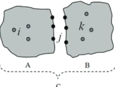
(2) Fig. 1 Coupling of sub-structures A and B, forming structure C From the equilibrium of forces and the compatibility conditions of displacements one can write:. fi A + fi B = fi C . . x =x =x A j. B j. . C j. (1) (2). The receptance matrices H relating the amplitudes of the forces to the amplitudes of the displacements are defined as (3). X = HF. and therefore, the receptance matrices for sub-structures A and B and for structure C are:. ⎡ H A HijA ⎤ H A = ⎢ iiA A⎥ ; ⎣⎢ H ji H jj ⎥⎦. . ⎡ H B H Bjk ⎤ H B = ⎢ Bjj B⎥ ; ⎣⎢ Hkj Hkk ⎥⎦. ⎡ HiiC ⎢ H C = ⎢ H Cji ⎢ HkiC ⎣. HijC H Cjj HkjC. HikC ⎤ ⎥ H Cjk ⎥ HkkC ⎥⎦. (4) . Using equations (1) and (2), one obtains the receptance matrix for C [11]:. ⎛ ⎡⎡ H A H A ⎤−1 0⎤ ⎡0 ij ⎜ ⎢ ii ⎥ ⎢ H C = ⎜ ⎢⎢⎢⎣ H jiA H jjA ⎥⎥⎦ 0⎥ + ⎢0 ⎜⎢ ⎥ ⎢ ⎜ 0 0 0⎦ ⎣0 ⎝⎣. . ⎡ H Bjj ⎢ B ⎢⎣ Hkj. −1. ⎤⎞ −1 ⎥ ⎟ H Bjk ⎤ ⎥ ⎟ ⎥ ⎟ HkkB ⎥⎦ ⎥⎦ ⎟ ⎠. 0 0. (5) . The process of inverting three matrices requires – in general – a high computational effort, implying a strong possibility of encountering ill-conditioned matrices. To try and minimize this problem an alternative formulation is often used [12]:. ⎡ HiiA HijA 0 ⎤ ⎡ HijA H −jj1 H jiA HijA H −jj1 H jjA −HijA H −jj1 H Bjk ⎤ ⎢ ⎥ ⎢ ⎥ H C = ⎢ H jiA H jjA 0 ⎥ − ⎢ H jjA H −jj1 H jiA H jjA H −jj1 H jjA −H jjA H −jj1 H Bjk ⎥ ⎢ 0 0 HkkB ⎥⎦ ⎢⎣−HkjB H −jj1 H jiA −HkjB H −jj1 H jjA HkjB H −jj1 H Bjk ⎥⎦ ⎣. . (6). A B where H jj = H jj + H jj . In a simpler way, one can write:. . ⎡ HiiC ⎢ C ⎢ H ji ⎢ HkiC ⎣. HijC H Cjj HkjC. HikC ⎤ ⎡ HiiA HijA 0 ⎤ ⎡ HijA ⎤ −1 ⎥ ⎢ ⎥ ⎢ ⎥ H Cjk ⎥ = ⎢ H jiA H jjA 0 ⎥ − ⎢ H jjA ⎥ ( H jjA + H Bjj ) ⎡⎣ H jiA H jjA −H Bjk ⎤⎦ HkkC ⎥⎦ ⎢⎣ 0 0 HkkB ⎥⎦ ⎢⎣−HkjB ⎥⎦. (7).

(3) which replaces the three inversions by only one, restricted to the number of connection co-ordinates j, thereby limiting possible numerical problems. 2.2 FRF uncoupling Let us suppose that our goal is the dynamic characterization of a joint; joints can be considered as complex components, often difficult to analyze and model. A possible solution relies on obtaining their dynamic behavior by an inverse coupling procedure, i.e., an uncoupling procedure, having eq. (7) as a starting point. If our joint is defined as sub-structure B, one has co-ordinates i and j, whereas co-ordinates k (internal to B) do not play a role here. Therefore, eq. (7) is re-written as:. . ⎡ HiiC HijC ⎤ ⎡ HiiA HijA ⎤ ⎡ HijA ⎤ A −1 =⎢ A − A ⎥ ( H jj + H Bjj ) ⎡⎣ H jiA H jjA ⎤⎦ ⎢ C C⎥ A⎥ ⎢ ⎣⎢ H ji H jj ⎦⎥ ⎢⎣ H ji H jj ⎦⎥ ⎢⎣ H jj ⎦⎥. (8). C. B C C From eq. (8) it is clear that there are three possibilities for the evaluation of H jj : using Hii , Hij or H jj .. 2.2.1 Without the use of co-ordinates j Sometimes it may be difficult to undertake measurements on co-ordinates j, close to the joint, so ideally one should use measurements on the complete structure C involving only co-ordinates i. From (8), one has:. HiiC = HiiA − HijA ( H jjA + H Bjj ) H jiA . . (9) . HijA ( H jjA + H Bjj ) H jiA = HiiA − HiiC . . (10) . . (11) . −1. Rearranging (9),. −1. . ( ). A Pre-multiplying (10) by Hij. −1. ( ). A and post-multiplying by H ji. (H. . A jj. + H Bjj ) = ( HijA ) −1. −1. −1. (H. A ii. leads to:. − HiiC )( H jiA ) −1. Note that this operation is mathematically possible only when i equals j; otherwise, if one of the (pseudo) inversions is B possible, the other one is not, and vice-versa. Solving for H jj , it follows that. H Bjj = H jiA ( HiiA − HiiC ) HijA − H jjA −1. . . (12) . Generalizing to the case where i might be different from j (in fact, i ≥ j ), one pre-multiplies equation (10) by an arbitrary matrix Wji and post-multiplies it by Wij :. Wji HijA ( H jjA + H Bjj ) H jiAWij = Wji ( HiiA − HiiC )Wij −1. . . (13) . . (14) . Rearranging eq. (13), one can write, . (H. A jj. + H Bjj ) = (Wji HijA ) Wji ( HiiA − HiiC ) Wij ( H jiAWij ) −1. −1. −1. This is only possible if i ≥ j , not the other way around (which certainly is not a common case). From (14) one has: . (. H Bjj = H jiAWij Wji ( HiiA − HiiC ) Wij. ). −1. Wji HijA − H jjA . . (15) .

(4) Now the order of the matrix to invert is equal to the number of co-ordinates j. This is advantageous because the size of j will be – in general – much smaller than that of i. The question is which matrix Wij to use. There is not an easy answer, but A. probably the most logical one is to use Hij :. (. H Bjj = H jiA HijA H jiA ( HiiA − HiiC ) HijA. . ). −1. H jiA HijA − H jjA . . (16) . . (17) . . (18). 2.2.2 Using only the coordinates of the joint C Using eq. (7) based on H jj , one has:. H Cjj = H jjA − H jjA ( H jjA + H Bjj ) H jjA −1. . B Solving eq. (17) with respect to H jj , it follows that:. (. ). H Bjj = H jjA ( H jjA − H Cjj ) − I jj H jjA . . −1. Based on the dynamic stiffness matrix of the structure, Ambrogio [1] obtains an alternative formulation (eq. (19) can be derived from eq. (18)):. (. H Bjj = I jj − H Cjj ( H jjA ). ). -1 −1. H Cjj . . (19) . HijC = HijA − HijA ( H jjA + H Bjj ) H jjA . . (20) . HijA ( H jjA + H Bjj ) H jjA = HijA − HijC . . (21). . (22). . (23). W ji HijA − H jjA . . (24). H jiA HijA − H jjA . . (25). . 2.2.3 Using coordinates i and j B Back again to eq. (8), the third option to evaluate H jj starts from: −1. or. −1. . Using once again arbitrary matrices, now W ji and W jj , with i greater or equal to j, one has. Wji HijA ( H jjA + H Bjj ) H jjA Wjj = Wji ( HijA − HijC ) Wjj −1. from which . (H. A jj. + H Bjj ) = (Wji HijA ) Wji ( HijA − HijC )Wjj ( H jjA Wjj ) −1. -1. -1. B Solving in order to H jj , gives:. . (. H Bjj = H jjA W jj W ji ( HijA − HijC )W jj. ). -1. A A As before, one shall make Wji = H ji and Wjj = H jj :. . (. H Bjj = H jjA H jjA H jiA ( HijA − HijC ) H jjA. ). -1.

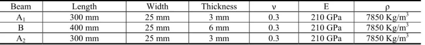
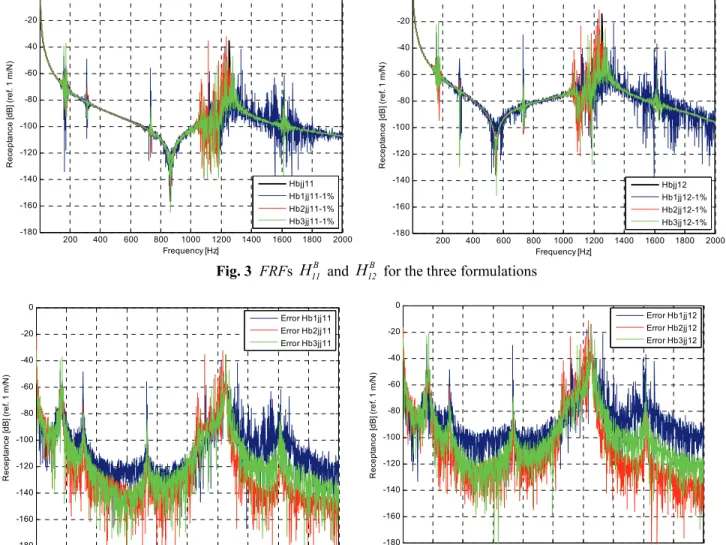
(5) 2.2.4 Summary B In summary, one has three formulations that allow us to determine matrix H jj : First formulation. (. H Bjj = H jiA HijA H jiA ( HiiA − HiiC ) HijA. Second formulation. (. ). −1. H jiA HijA − H jjA . . (16) . ). . (18). H jiA HijA − H jjA . . (25). H Bjj = H jjA ( H jjA − H Cjj ) − I jj H jjA . Third formulation. −1. (. H Bjj = H jjA H jjA H jiA ( HijA − HijC ) H jjA. . ). -1. 3 SIMULATION STUDIES To illustrate the performance of the three formulations one uses the beam of figure 2, constituted by three components, A1, B and A2, forming structure C; A1 and A2 form sub-structure A. 1. 3. 5 4. 2. 7 6. i. 9. j. A1. 15. 13. 11. 10. 8. 12. 14. 16. 18. 20. i. j. B. 19. 17. A2. Fig. 2 Test item B. A. C. The aim is to characterize component B (our “joint”), evaluating H , assuming that H is calculated analytically and H is calculated through experiments (simulated, in this case). Using the finite element method with beam elements with four degrees of freedom, each component is divided into eight elements and considering only the nodes shown in figure 2 as coordinates i and j where it is possible to measure and excite the structure. The characteristics of each component are displayed in table 1.. Beam A1 B A2. Length 300 mm 400 mm 300 mm. Table 1 Characteristics of the components of the beam Width Thickness E ν 25 mm 3 mm 0.3 210 GPa 25 mm 6 mm 0.3 210 GPa 25 mm 3 mm 0.3 210 GPa. ρ 7850 Kg/m3 7850 Kg/m3 7850 Kg/m3. 3.1 Choice of the formulation C To simulate the experimental errors, one has imposed a 1% perturbation in matrix H for the three formulations. The B elements 11 and 12 (chosen just for comparison) of matrix H jj obtained with the three formulations are shown in figure 3.. The major disturbances in the responses are due to numerical problems in the matrix inversions in each of the formulations. The variability of the results in figure 3 is quite high. Figure 4 represents the module of the differences between the numerically exact response and the response obtained by the three formulations. From the three results, the second formulation is the one that produces the smallest error throughout the frequency range..

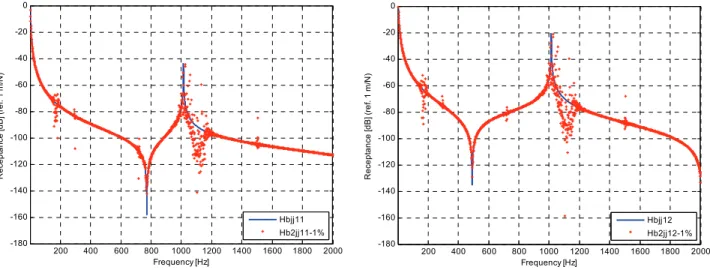
(6) 0. -20. -20. -40. -40 Receptance [dB] (ref. 1 m/N). Receptance [dB] (ref. 1 m/N). 0. -60 -80 -100 -120 -140 -160 -180. 200. 400. 600. 800 1000 1200 Frequency [Hz]. 1400. -60 -80 -100 -120. Hbjj11 Hb1jj11-1%. -140. Hb2jj11-1% Hb3jj11-1%. -160. 1600. 1800. Hbjj12 Hb1jj12-1% Hb2jj12-1% Hb3jj12-1%. -180. 2000. 200. 400. 600. 800 1000 1200 Frequency [Hz]. 1400. 1600. 1800. 2000. B B Fig. 3 FRFs H11 and H12 for the three formulations 0. 0. Error Hb1jj12. Error Hb1jj11 Error Hb2jj11 Error Hb3jj11. -20. Receptance [dB] (ref. 1 m/N). Receptance [dB] (ref. 1 m/N). Error Hb3jj12. -40. -40 -60 -80 -100 -120. -60 -80 -100 -120. -140. -140. -160. -160. -180. Error Hb2jj12. -20. -180. 200. 400. 600. 800 1000 1200 Frequency [Hz]. 1400. 1600. 1800. 2000. 200. 400. 600. 800 1000 1200 Frequency [Hz]. 1400. 1600. 1800. 2000. B B Fig. 4 Errors of FRFs H11 and H12 for the three formulations. 0. 0. -20. -20. -40. -40 Receptance [dB] (ref. 1 m/N). Receptance [dB] (ref. 1 m/N). B B Let us represent H11 and H12 only for the second formulation, superimposed with the numerically exact response (see figure 5).. -60 -80 -100 -120. -60 -80 -100 -120 -140. -140 -160. -160. Hbjj11. Hbjj12 Hb2jj12-1%. Hb2jj11-1% -180. 200. 400. 600. 800 1000 1200 Frequency [Hz]. 1400. 1600. 1800. 2000. -180. 200. 400. 600. 800 1000 1200 Frequency [Hz]. B B Fig. 5 H11 and H12 for the second formulation. 1400. 1600. 1800. 2000.

(7) 3.2 Strategies to improve the results It is clear that one cannot be happy with the results of figure 5. Let us try to improve them. From eq. (18) it is apparent that. (. ). A C the problems certainly arise in the inversion of H jj − H jj , namely when this difference is small. To try to increase this. difference one will change our structure by adding point masses, so to change the behavior of sub-structure A and C, while B remains unchanged.. 0. 0. -20. -20. -40. -40 Receptance [dB] (ref. 1 m/N). Receptance [dB] (ref. 1 m/N). 3.2.1 Adding mass to sub-structure A B B A mass of 35 grams has been added to nodes 1, 3, 5 and 15, 17, 19. The new results for H11 and H12 are shown in figure 6.. -60 -80 -100 -120. -60 -80 -100 -120 -140. -140 -160. -160. Hbjj11. Hbjj12 Hb2jj12-1%. Hb2jj11-1% -180. 200. 400. 600. 800 1000 1200 Frequency [Hz]. 1400. 1600. 1800. -180. 2000. 200. 400. 600. 800 1000 1200 Frequency [Hz]. 1400. 1600. 1800. 2000. B B Fig. 6 H11 and H12 with added masses in sub-structure A. It can be observed from figure 6 that the disturbance observed between 1000-1200 Hz in figure 5 moves into the range 8001000 Hz, generally improving the results.. 0. 0. -20. -20. -40. -40 Receptance [dB] (ref. 1 m/N). Receptance [dB] (ref. 1 m/N). 3.2.2 Adding mass to sub-structure B An alternative could be to add mass to the sub-structure B itself. Adding 35 grams at co-ordinates j = 9 and 11, leads to the results presented in figure 7.. -60 -80 -100 -120 -140. -60 -80 -100 -120 -140. -160. -160. Hbjj11. Hbjj12. Hb2jj11-1% -180. 200. 400. 600. 800 1000 1200 Frequency [Hz]. 1400. 1600. 1800. 2000. Hb2jj12-1% -180. 200. 400. 600. 800 1000 1200 Frequency [Hz]. 1400. 1600. 1800. 2000. B B Fig. 7 H11 and H12 with added masses of 35 grams in sub-structure B. As sub-structure B is altered, its natural frequency (identified in figure 5) changes to the left. However, the disturbances remain in the area of 1000-1200 Hz and one can conclude that they are caused caused by sub-structure A. So maybe one can improve the results by adding some more mass to sub-structure B, to cause the natural frequency to deviate from the disturbance. Let us now add masses of 70 grams. The results are displayed in figure 8..

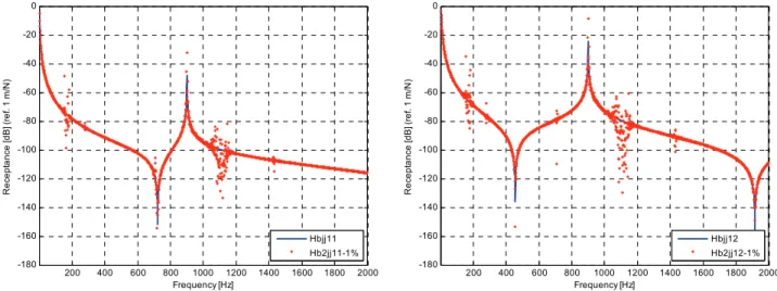
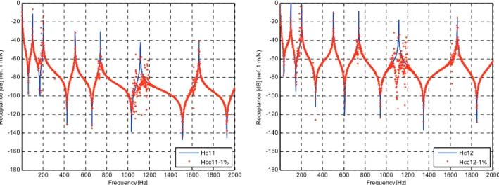
(8) 0. -20. -20. -40. -40 Receptance [dB] (ref. 1 m/N). Receptance [dB] (ref. 1 m/N). 0. -60 -80 -100 -120 -140. -60 -80 -100 -120 -140. -160. -160. Hbjj11. Hbjj12. Hb2jj11-1% -180. 200. 400. 600. 800 1000 1200 Frequency [Hz]. 1400. 1600. 1800. 2000. Hb2jj12-1% -180. 200. 400. 600. 800 1000 1200 Frequency [Hz]. 1400. 1600. 1800. 2000. B B Fig. 8 H11 and H12 with added masses of 70 grams in sub-structure B. The results are clearly better. However, to recover the dynamic response of B, one has to uncouple the added masses. The results of such an operation are shown in figure 9.. B B Fig. 9 H11 and H12 with and without the masses of 70 grams in sub-structure B. Although the results are better than the initial ones (figure 5), they are worse than those of figure 6, when the masses were added to sub-structure A. The disturbances come up again in the same frequency range. 3.3 Coupling One of the main interests of the dynamic characterization of a sub-structure (like a joint) is to be able to predict the dynamic behavior of another structure (or a modified one), possibly a more complex one, inserting (coupling) the identified results from the uncoupling procedure. Whereas the uncoupling procedure tends to be unstable, as shown in this work, the coupling process is usually quite stable. Based on the results obtained for sub-structure B, a coupling procedure will be undertaken with similar components, two beams A1 and A2 but now with a length of 400 mm. Using the results initially obtained from figure 5, one obtains the behavior illustrated in figure 10. In figure 10 the disturbance in the area of 1000-1200 Hz remains. One can also observe the results of the coupling of B when the masses were added to A, i.e., when using the responses given in figure 6. Figure 11 illustrates this case. The results have improved and the disturbances have moved down, as expected. Most certainly, better solutions would have been obtained if one had performed a modal analysis identification to the results of figure 6, prior to the coupling procedure..

(9) 0. -20. -20. -40. -40 Receptance [dB] (ref. 1 m/N). Receptance [dB] (ref. 1 m/N). 0. -60 -80 -100 -120 -140. -60 -80 -100 -120 -140. -160. -160. Hc11. Hc12. Hcc11-1% -180. 200. 400. 600. 800 1000 1200 Frequency [Hz]. 1400. 1600. 1800. 2000. Hcc12-1% -180. 200. 400. 600. 800 1000 1200 Frequency [Hz]. 1400. 1600. 1800. 2000. 0. 0. -20. -20. -40. -40 Receptance [dB] (ref. 1 m/N). Receptance [dB] (ref. 1 m/N). C C Fig. 10 H11 and H12 resulting from the coupling of A1 and A2 with the sub-structure B. -60 -80 -100 -120. -60 -80 -100 -120 -140. -140 -160. -160. Hc11-1%. Hc12-1% Hcc12-1%. Hcc11-1% -180. 200. 400. 600. 800 1000 1200 Frequency [Hz]. 1400. 1600. 1800. 2000. -180. 200. 400. 600. 800 1000 1200 Frequency [Hz]. 1400. 1600. 1800. 2000. C C Fig. 1 H11 and H12 resulting from the coupling of A1 and A2 with the sub-structure B, with the addition of masses in A. 4 CONCLUSIONS In this paper the authors have presented three formulations for the uncoupling of sub-structures, something that may be of considerable interest, for instance when trying to model complex joints. The formulation that presented the best results requires measurements at the connection points of the structures; unfortunately, this may not always be possible in practice. Any of the three formulations revealed to be numerically unstable due to the inversion of difference matrices. This problem has been investigated in this study and improvements have been obtained when adding point masses to the remaining substructures other than the one to be characterized. Those added masses move the natural frequencies, allowing to understand the problems that are happening and as already said, improving the results. Together with the use of modal identification methods, the uncoupling techniques may be of interest in various situations. Experimental implementation still has to be further investigated, as the accurate measurement of rotations is quite difficult to obtain. REFERENCES [1] D'Ambrogio, W., Fregolent, A. "Sensitivity of decoupling techniques to uncertainties in the properties" Proceedings of "Noise and Vibration Engineering" (ISMA 2008), Leuven, Belgium, pp. 3737-3749, 2008..

(10) [2] Rixen, D. J. "A dual Craig-Bampton method for dynamic substructuring" Journal of Computational and Applied Mathematics, Vol. 168, pp. 383 – 391, 2004. [3] Craig, R., Bampton, M. "Coupling of Substructures for Dynamic Analysis" AIAA Journal, vol. 6, pp. 1313 – 1319, 1968. [4] Ahmadian, H., Hadad, H. "Identification of a Bolted Lap Joint Parameters Using Response Surface Method" Proceedings of "Noise and Vibration Engineering" (ISMA 2006), Leuven, Belgium, pp. 1259-1272, 2006. [5] Jalali, H., Ahmadian, H., Mottershead, J.E. "Identification of nonlinear bolted lap-joint parameters by force-state mapping" International Journal of Solids and Structures, Vol. 44, Issues 25-26, pp. 8087-8105, 2007. [6] Jetmundesn, B., Bielawa, R., Flannelly, W.G. "Generalized Frequency Domain Substruture Synthesis" Jounal of the American Helicopter Society, Vol. 33, pp. 55–64, 1988. [7] de Klerk, D., Rixen, D. J., Voormeeren, S. N. "General Framework for Dynamic Substructuring: History, Review, and Classification of Techniques" Journal American Institute of Aeronautics and Astronautics, vol. 46 (5), pp.1169-1181, 2008. [8] Ren, Y., Beards, C. F. "A new method for the identification of joint proprites using FRF data" Proceedings of the Florence Modal Analysis Conference, Italy, pp. 663-669, 1991. [9] Maia, N.M. M., Silva, J. M. M., Ribeiro, A. M. R, Silva, P. L.C. G. C. "On the dynamic characterization of joints using uncoupling techniques " Proc. of the 16th International Modal Analysis Conference (IMAC XVI), Sta. Barbara, U.S.A, pp. 1132-1138, 1998. [10] Urgueira, A.P V. Dynamic analysis of coupled structures using experimental data Ph.D. Thesis, Imperial College of Science Technology and Medicine, London, 1989. [11] Maia, N. M. M., Silva, J. M. M. et al. "Theoretical and Experimental Modal Analysis" Research Studies Press, Distrib. John Wiley & Sons, pp. 480, 1997. [12] Skingle, G.W. Structural Dynamic Modification Using Experimental Data Ph.D Thesis, Imperial College of Science Technology and Medicine, London, 1989..

(11)