1. INTRODUCTION
Current research aims to understand the modelling properties of the various Artificial Neural Networks (ANN) architectures. New algorithms are being developed to improve their fitness for modelling and control applications. Different architectures can be found in the literature, however, B-spline neural networks offer definite advantages over more commonly known neural networks, such as multilayer perceptrons or radial basis function networks. One of the most important advantage is its suitability for on-line adaptive modelling and control applications. Their grid-based structure makes them transparent, which, in contrast to other networks, means that it is easier to understand the knowledge stored in these networks (this is an advantage that is also applies to fuzzy rule-based models over conventional neural networks). It is not surprising that, at a high level, the basic information principles of B-spline networks and fuzzy systems are the same. So, under certain conditions, the low-level algorithms are also identical. For fuzzy systems, the most important task is to find the optimal rule base; this is translated, in terms of BNNs in the determination of the best topology and its parameters values. The rule
base might be given by a human expert or might be given a priori by the linguistic description of the modelled system. If neither is available, the system has to be designed by other methods based on numerical data.
Nature inspired some evolutionary optimisation algorithms suitable for global optimisation of even non-linear, high-dimensional, multimodal, and discontinuous problems. The original genetic algorithm (GA) was developed by Holland (Holland, 1992) and was based on the process of evolution of biological organisms. Recently, approaches like genetic programming and bacterial evolutionary algorithm present an alternative to the former algorithms. GP optimisation uses the same operators as GA, though it requires an expression tree for gene representation as a combination of functions. The BEA is a simpler algorithm, and its operations were inspired by the microbial evolution phenomenon. The current paper focuses on a comparison between the applicability of GP for BNN design and BEA for the optimisation of the fuzzy rule base.
The layout of the paper is as follows: Section 2 and 3 introduce the topology of B-spline neural networks and the Fuzzy Systems concept. In Section 4 and 5 GP for BNN and BEA for fuzzy rule extraction will
GENETIC PROGRAMMING AND BACTERIAL ALGORITHM FOR
NEURAL NETWORKS AND FUZZY SYSTEMS DESIGN
C. Cabrita12, J. Botzheim3, A. E. Ruano12, L. T. Kóczy34
1. ADEEC, FCT, Universidade do Algarve
Campus de Gambelas, 8000 Faro, Portugal 2. Centro de Sistemas Inteligentes, Portugal 3. Department of Telecommunication and Telematics, Budapest University of Technology and Economics.
4.Institute of Information Technology and Electrical Engineering, Széchenyi István University, Győr, Hungary
emails: [email protected], [email protected], [email protected], [email protected]
Abstract – In the field of control systems it is common to use techniques based on model
adaptation to carry out control for plants for which mathematical analysis may be intricate. Increasing interest in biologically inspired learning algorithms for control techniques such as Artificial Neural Networks and Fuzzy Systems is in progress. In this line, this paper gives a perspective on the quality of results given by two different biologically connected learning algorithms for the design of B-spline neural networks (BNN) and fuzzy systems (FS). One approach used is the Genetic Programming (GP) for BNN design and the other is the Bacterial Evolutionary Algorithm (BEA) applied for fuzzy rule extraction. Also, the facility to incorporate a multi-objective approach to the GP algorithm is outlined, enabling the designer to obtain models more adequate for their intended use. Copyright 2003 IFAC.
Keywords: constructive algorithms, B-splines, genetic programming, bacterial evolutionary algorithm, fuzzy rule base;
be described. Results are presented in Section 6 and conclusions are drawn in Section 7.
2. B-SPLINENEURALNETWORKS
B-spline neural networks belong to the class of networks termed grid or lattice-based associative
memories networks (AMN). This type of networks is
composed of three layers: a normalised input space layer, a basis functions layer and a linear weight layer.
2.1. Normalised Input Layer
The normalised input layer can take different forms but is usually a grid on which the basis functions are defined. To define a grid, vectors of knots must be defined, one for each input axis. There are usually a different number of knots for each dimension, and they are generally placed at different positions. The interior knots, for the ith axis, are λi j, ,j=1,L,ri.
They are arranged in such a way that:
min max ,1 , 2 ,i i i i i r i x <λ ≤λ ≤L≤λ <x , (1) where min i x and max i
x are the minimum and maximum values of the ith input, respectively.
At each extreme of each axis, a set of ki exterior knots must be given which satisfy:
( ) ,0 min , i 1 i i i k x λ − − ≤L≤λ = (2) max ,i 1 ,i i i i r i r k x =λ + ≤L≤λ + (3)
These exterior knots are needed to generate the basis functions that are close to the boundaries.
The jth interval of the ith input is denoted as Ii,j and is defined as: , 1 , , , 1 , 1, , 1 i j i j i i j i j i j i for j r I if j r λ λ λ λ − − = = = + L (4)
This way, within the range of the ith input, there are
ri+1 intervals (possibly empty if the knots are coincident), which means that there are
(
)
1 1 n i i p r = = +′
∏
n-dimensional cells in the grid.2.2. The basis functions layer
The output of the hidden layer is determined by a set of p basis functions defined on the n-dimensional grid. The univariate B-spline basis function of order k has a support, which is k intervals wide. Hence, each input is assigned to k basis functions.
The jth univariate basis function of order k is denoted ( )
j k
N x , and it is defined by the following relationships: 1 1 1 1 1 ( ) j k ( ) j ( ) j j j k k k j j k j j k x x N x λ N x λ N x λ λ− −− λ λ − − − − + − − = + − − (5) 1 1 ( ) 0 j j if x I N x otherwise ∈ = (6)
Multivariate basis functions are formed by taking the
tensor product of the univariate basis functions.
The number of basis functions of order ki defined on an axis with ri interior knots is ri+ki. Therefore, the total number of basis functions for a multivariate
B-spline is
(
)
1 n i i i p r k = =∏
+ .This number depends exponentially on the size of the input and because of this, B-splines are only applicable for problems where the input dimension is small (typically ≤5).
2.3. The weight layer
The output of an AMN is a linear combination of the outputs of the basis functions. The linear coefficients are the adjustable weights, and as the mapping is linear, finding the weights is just a linear optimisation problem. The output is therefore:
1 p T i i i y = =
∑
a w =a w, (7) 2.4. Sub-ModulesTo overcome the “curse of dimensionality”, it is common to employ, instead of a single module covering all inputs, a linear sum of smaller sub-modules, each one with a lower input dimensionality. The output of such a network is:
( )
( )
1 u n u u u y S = =∑
x x (8)where S xi
( )
i denotes the i thsub-model, and xi is the
set of input variables (i) which compose sub-model
i.
3. FUZZYSYSTEMS
The theory of fuzzy logic was first proposed by Zadeh in the 1960s. His main idea was that most of the phenomena of the real world could not be described by two values, so he defined a function which would assign fuzzy truth degrees between zero and one to elements of a universal set. In 1973 he pointed out that the new fuzzy concept could be excellently used for describing very complex problems with a system of fuzzy relations represented by a fuzzy rule base [1].
A fuzzy rule base contains fuzzy rules that map the multivariate fuzzy input set to the univariate output set. Let’s denote a rule by Ri,:
Ri: IF (x1 is Ai1) AND (x2 is Ai2) AND
... AND (xn is Ain) THEN (y is Bi), (9)
where Aij and Bi are fuzzy sets, xj and y are the fuzzy inputs and output, respectively.
The structure of a rule is the following:
where the premise consists of antecedents linked by the AND operator.
To implement a rule set, each of the univariate fuzzy linguistic statements – e.g. (xn is Ain) – needs to be given and also the operators used to implement the underlying fuzzy logic, such as AND, THEN, etc., need to be specified. Because no single implementation is correct, many implementation methods have been proposed (Harris et al., 1993). A crisp input is presented to the network, and the membership functions of the multivariate fuzzy input linguistic variables are computed. The network output is obtained by defuzzifying this information.
3.1. RELATIONS BETWEEN FUZZY SYSTEMS
AND B-SPLINE NETWORKS MODELS
In the simplest form, fuzzy systems calculate their response by taking a linear combination of the input membership functions, in an analogous way as several neural networks. The relationships between fuzzy and B-spline networks, have been addressed by several authors (see, for example (Nelles, 2000; Ruano et al., 2001)). In order to have a strict equivalence between FS and BNN models, the FS must satisfy some assumptions, which are outlined in (Ruano et al., 2001). In the current work, the structure of the Mamdani FS and BNN models are not strictly equivalent, their main differences being:
• The linguistic terms of the rule antecedents and consequents are not modelled by
B-splines, instead, by trapezoids.
• For the logic connectives such as the conjunction and implication, the t-norm used is not the algebraic product, but the
min operator;
Please note that it is not essential that the two model’s structures are equivalent, since the main objective of this work is the comparison of the performance between two different optimisation heuristics and not a structure comparison.
4. GENETICPROGRAMMING
Genetic programming employs the main operators used by a genetic algorithm in its search procedure. The main difference, which, from our point of view is beneficial for this type of neural networks, is that the network parameters are not coded as bit strings, but instead as a tree structure, composed of function and terminal nodes, is employed. The tree structure, as well as the characteristics of the nodes, evolves from generation to generation.
4.1. Single Objective Genetic Programming
For the case of B-Spline construction, and referring to the previous sections, sub-models must be added (+), sub-models of higher dimensionality must be
created from smaller modules (*), and
sub-models of higher dimensionality must be split into lower dimensional sub-models (/). These are the set of primitive functions that were implemented. In contrast with the application of GP to other neural networks, the node terminals do not represent only each input variable, but also the spline order, the
number of interior knots, and their location.
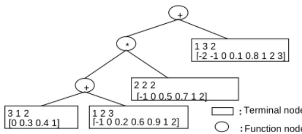
An example of an expression tree for B-spline networks is presented in the next figure.
Fig 1: A sample expression tree for B-spline networks.
The evolutionary process involves the following steps:
• The creation of an initial population, and the determination of the size of the population;
• The evaluation of the candidates using
Bayes Information Criterion (Nelles, 2001), and their fitness assignment;
• The application of genetic operations, such as:
! Selection: Pairs of parent trees are selected based on their fitness for reproduction;
! Crossover: A node in the tree is selected at random and exchanging the associated sub-trees produces a pair of offspring sub-trees.
! Mutation: This is performed by either replacing a node selected at random by a sub-tree generated randomly or by changing its type.
! Replacement: All parents are replaced by the offspring (generational approach).
• The termination criterion, which is usually the maximum number of generations defined.
The evolution cycle is summarized in Figure 2. Mutation on a function implies the replacement of the tree node with a randomly generated sub-tree of maximum length 2. Mutation on a terminal can be of 6 different types, which are:
1. Full replacement of the terminal. 2. Variable identification replacement. 3. Splines order replacement.
4. Random displacement of an interior knot. 5. Addition of N interior knots placed
randomly. N is fixed to 5.
6. Removal of N interior knots. In the absence of interior knots, no operation is executed.
For simplification purposes, the terminal mutation rates will be described as a vector p_m_terminal=[%1 %2 %3 %4 %5 %6], where %i designates the ith type mutation rate.
+ * + 1 3 2 [-2 -1 0 0.1 0.8 1 2 3] 1 2 3 [-1 0 0.2 0.6 0.9 1 2] 3 1 2 [0 0.3 0.4 1] 2 2 2 [-1 0 0.5 0.7 1 2] : Terminal node : Function node
For a more detailed explanation, please see (Cabrita, et al., 2001). Initial Population Creation Candidates evaluation Fitness assignment n=N? Generate new population show best candidate n=n+1 n=1
Fig 2: Flowchart for Genetic Programming.
4.2. Multi-objective genetic programming
GP can also be applied in a multi-objective strategy, which is useful for B-spline networks design. For a description on multi-objective optimisation, please refer to (Fonseca, 1998).
In this approach, candidate evaluation consists not only of the objective functions evaluation, but also of a decision process based on priorities and goals associated with every objective. At each generation, fitness is assigned to the candidates according to the result of that decision process. Non-dominated solutions are recorded, and in the end, the decision maker selects the best non-dominated solutions that correspond to the preferred candidates.
Here, the following objectives have been considered:
• Mean Square of Absolute Error for training and validation data (MSE/MSEv).
• Mean Square of Relative Error for training and validation data (MSRE).
2 _ 2 1 ( ) 1 ; _ N pat i i i i t y MSRE N pat = y − =
∑
• Mean of Relative Error Percentage for training and validation data (PMRE/PMREv). _ 1 100 . _ N pat i i i i t y PMRE N pat = y − =
∑
Some objectives may have greater priority than others. Objectives with priority greater than 0, together with the corresponding goals, act as constraints that must be satisfied. Lower-priority objectives are only taken into account as long as the remaining ones have their goals satisfied.
5. BACTERIALEVOLUTIONARY
ALGORITHM
A newer approach is the bacterial algorithm. This is based on a process, which can be found in nature. Bacteria can transfer genes to other bacteria. This mechanism is used in the bacterial mutation and in the gene transfer operation. The gene transfer
operation substitutes the GA’s crossover operation, so the information can be transferred between different individuals (Nawa and Furuhashi, 1999).
5.1. The encoding method
Referring now to Section 3, for a fuzzy system design using BEA, the class of membership function is restricted to a trapezoidal function, described by its four breakpoints. The membership functions are identified by the two indices i and j, so that, the membership function Ai,j(xj) belongs to the ith rule and the jth input variable. Bi(y) is the output membership function of the ith rule and its shape is the same as for Ai,j(xj) but it is described by different breakpoints (Botzheim, 2001).
The encoding method of a fuzzy system with two inputs and one output, can be observed in Fig. 3.
Fig 3: Fuzzy rules encoded in a chromosome.
For example, Rule 3 in Fig. 3 means:
If x1 is A31 and x2 is A32 then y is B3 (11)
where A3,1 A3,2 and B3 mean the trapezoidal membership function with the breakpoints values shown in the previous figure.
5.2. The algorithm
Generating the initial population. First, the initial bacteria population is created randomly. The population consists of n chromosomes (the bacteria). The initial number of rules in one chromosome is
Nmax. So, n(k+1)Nmax membership functions are created, where k is the number of input variables in the given problem, and each membership function has four parameters.
Bacterial mutation The bacterial mutation is applied to each chromosome one by one as in (Nawa and Furuhashi, 1999). First, m -1 copies (clones) of the rule base are generated. Then a certain part of the chromosome is randomly selected and the parameters of this selected part are randomly changed in each clone (mutation). Next, all the clones and the original bacterium are evaluated by the error criterion. The best individual transfers the mutated part into the other individuals. This cycle is repeated for the remaining parts, until all parts of the chromosome have been mutated and tested. At the end, the best rule base is kept and the remaining m -1 are discharged.
Gene transfer operation. The gene transfer operation allows the recombination of genetic information between two bacteria.
First, the population must be divided into two halves. The better bacteria are called superior half, the other bacteria are called inferior half.
One bacterium is randomly chosen from the superior half, this will be the source bacterium, and another is randomly chosen from the inferior half, this will be the destination bacterium.
A “good” part from the source bacterium is chosen and this part can overwrite a not-so-good part of the destination bacterium or simple be added. A good part can be a fuzzy rule with a high degree of activation value. The activation value of a fuzzy rule is calculated as follows: ( ) 1 1 P j i i j w w P = =
∑
(12)where
w
i is the mean activation value of thei
thrule,) ( j
i
w
is the activation value of thei
thrule for the thj
pattern, P is the number of patterns. So the best part of the source bacterium is the rule which has the greatest mean activation value.Gene transfer is repeated for
N
inftimes, whereinf
N
is the number of “infections” per generation. Stop condition. If the population satisfies a stop condition or the maximum generation number is reached, then the algorithm ends. Otherwise it returns to the bacterial mutation step.5.3. Definition of the error function
The error function used for training is defined as follows: max min ˆ 1 rel patterns y y e n I I − = −
∑
(13)where Imax is the upper and Imin is the lower bound of the interval of the output variable, so the error is normalised by the length of the output interval rather than the actual value of the output.
6. RESULTS
Three different examples have been experimented with GP and BEA. Both algorithms were set to run for 10 sessions of 40 generations and the results obtained relate to the following specifications: Mean
Square of the absolute Error, Mean Square of the
Relative Error, Mean Relative Error Percentage,
and structure Complexity (number of basis functions) for both training and validation data (using v subscript). The training and validation sets contained the same number of patterns and some of the patterns were identical. 110 patterns were used for the pH problem, 101 patterns for the ICT problem and 200 patterns for the six-dimensional generic function. For GP, the population size is 10, the initial population creation method is ramped-half-and-half,
the fitness assignment is exponential ranking with selective pressure 5, and the crossover rate, the mutation rate and the number of generations are 0.5, 0.8, 40, respectively. The terminal mutation rate is [5% 10% 5% 10% 60% 10%].
For BEA, the population size and number of clones are 10, the number of infections and rules is 5 and 7, respectively.
6.1. pH problem
The aim of this example is to approximate the inverse of a titration-like curve. This type of non-linearity relates the pH (a measure of the activity of the hydrogen ions in a solution) with the concentration (x) of chemical substances.
6.2 Inverse Coordinate Transformation Problem
(ICT)
This example illustrates an inverse kinematic transformation between 2 Cartesian coordinates and one of the angles of a two-links manipulator.
For a more complete description on the above examples refer to (Ruano et. al, 2001).
6.3 A sixth input generic function
This example is widely used as a target function and the output is given by the following expression (see Botzheim et. al, 2001):
5 6 2( ) 0.5 1 2 3 4 2 x x y= +x x +x x + e − (14)
6.4 Comparison between SOGP and Bacterial
Algorithm
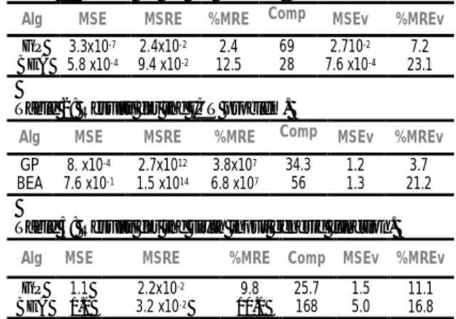
The values shown from Table 1 to Table 4 refer to results obtained from the 10 different sessions, and show mean values of specifications for the best candidates from each run, for the PH, ICT and sixth input generic function, respectively.
Table 1: Results for the PH problem.
Alg MSE MSRE %MRE Comp MSEv %MREv
GP BEA 3.3x10⁻⁷ 5.8 x10⁻⁴ 2.4x10⁻² 9.4 x10⁻² 2.4 12.5 69 28 2.710-2 7.6 x10⁻⁴ 7.2 23.1
Table 2: Results for the ICT problem.
Alg MSE MSRE %MRE Comp MSEv %MREv
GP BEA 8. x10-4 7.6 x10⁻¹ 2.7x10¹² 1.5 x10¹⁴ 3.8x10⁷ 6.8 x10⁷ 34.3 56 1.2 1.3 3.7 21.2
Table 3: Results for the sixth input generic function.
Alg MSE MSRE %MRE Comp MSEv %MREv
GP BEA 1.1 1.1 2.2x10⁻² 3.2 x10⁻² 9.8 10.1 25.7 168 1.5 5.0 11.1 16.8
From the previous tables, it can be observed that, with the exception of the pH problem, GP optimising the BNN results in better accuracy between the desired output and estimated output, than the BEA
does for the FS rule extraction, for all the specifications,. The results from the validation set uphold the training values and sometimes, as is the case of the ICT problem, present lower specification values. It can also be seen that the complexity of the structure is important, because it gives an idea about the generalisation capabilities of the models: in general, the lower is the complexity, the better the generalisation capability.
6.5 Multi-objective GP approach
Supposedly the mean values for the training data for GP, in Table 2 are not as good as expected. A way of establishing a compromise between the training and validation set specifications is using the multi-objective approach for the ICT problem. It should be stressed that this could also be done with any of the other problems. 10 sessions were executed using the parameters in Table 4. Every non-dominated solution from every session was saved and in the end, the decision maker showed the preferred solutions from all the sessions based on the goal and priorities vector shown in the 3rd and 4th column.
Table 4: Multi-objective parameters specification for ICT Numb. Individuals Numb. Generations Priority Vector Goal Vector 10 40 [1 2 2 0 0] [10-4 105 103 10-4 10-2] 1 2 3 4 5 CO S T OBJECTIVE NUMBER
Fig 4: Best trade-off curve for the ICT problem.
The results shown in Fig. 4 allow the designer to deduce that it is possible to get good models simultaneously, for the training and validation set, as is the case. Please note that the values in the 3rd column represent the position of the crosses, i.e, approximately the values obtained for each objective. The specifications for the training data have been optimised and its values are much lower than the goals set. One should emphasize that this is not always the case because some other conflicting objectives can be imposed, for e.g. the complexity of the network (the preferred solution presented shows a complexity value of 56) or the condition of the model.
7. CONCLUSIONS
Two recent new methodologies for optimising the structure of neural networks and fuzzy models were subject to comparison. It was observed that the output accuracy attained with the neural network structure, optimized with GP, was better than the one achieved with the fuzzy system, optimized by BEA. One can deduce it might be from the fuzzy structure, which is not identical to the BNN, however, from the point of view of modelling, if the model from the NN and FS are to be seen as a black box, then the GP has better performance. Also, the facility to incorporate a multi-objective approach in GP allows the designer the freedom to obtain models more adequate to their intended use.
As future work, it may be helpful to try and use GP for FS optimisation or to use BEA to optimise a FS whose structure is identical to the BNN, or to optimise the BNN structure itself.
ACKNOWLEDGEMENTS
Research supported by the Nationals Scientific Research Fund OTKA T034233 and T034212, a Széchenyi University Research Grant 2002, the National Research and Development Project Grant 2/0015/2002 and by the bilateral ICCTI-OMFB 4.1.1 research cooperation grant.
REFERENCES
Botzheim, J., Hámori, B., Kóczy, L. T., (2001) Extracting trapezoidal membership functions of a fuzzy rule system by bacterial algorithm, 7th Fuzzy Days, Dortmund, Springer-Verlag, pp. 218-227
Cabrita, C., Fonseca, C. M., Ruano, A. E., (2001) Single and multi-objective genetic programming design for B-spline neural networks and neuro-fuzzy systems, submitted to IFAC, Valencia.
Fonseca, C. M.,Fleming, P.J. (1998a) Multiobjective
optimization and multiple constraint handling with evolutionary algorithms I: A unified formulation, IEEE Transactions on SMC, Part A, 28, (1) 26-37
Harris, C.J., Moore C.G., Brown M. (1993) Intelligent Control: Some Aspects of Fuzzy Logic and Neural Networks, World Scientific Press, London & Singapore.
Holland, J. H., (1992) Adaptation in Nature and Artificial Systems: An Introductory Analysis with Applications to Biology, Control, and Artificial Intelligence, MIT Press, Cambridge.
Nawa, N. E., Furuhashi, T., (1999) Fuzzy System Parameters Discovery by Bacterial Evolutionary Algorithm, IEEE Tr. Fuzzy Systems 7, pp. 608-616.
Nelles, O., (2000), Nonlinear Systems Identification with Local Linear Neuro-Fuzzy Models, PhD. Thesis, TU Darmstadt, Germany
Ruano A. E., C. Cabrita, J. V. Oliveira, L. T. Kóczy, (2001) Supervised training algorithms for B-spline neural networks and neuro-fuzzy systems, submitted to International Journal of Systems Science
Zadeh, L. A., (1973) Outline of a new approach to the analysis of complex systems and decision processes, IEEE Tr. Systems, Man and Cybernetics 3, pp. 28-44.

![Table 4: Multi-objective parameters specification for ICT Numb. Individuals Numb. Generations Priority Vector Goal Vector 10 40 [1 2 2 0 0] [10 -4 10 5 10 3 10 -4 10 -2 ] 1 2 3 4 5COST OBJECTIVE NUMBER](https://thumb-eu.123doks.com/thumbv2/123dok_br/18638064.911621/6.918.102.446.497.807/objective-parameters-specification-individuals-generations-priority-vector-objective.webp)
