Hydrodynamic Optimization of a torpedo-shaped hull

(1)

Engenharia

Hydrodynamic Optimization of

a torpedo-shaped hull

Tiago Correia Bartolomeu

Dissertação para a obtenção do Grau de Mestre em

Engenharia Aeronáutica

(Ciclo de estudos integrado)

Orientadores: Ph.D. Francisco Miguel Ribeiro Proença Brójo

M.Sc. Paulo de Vasconcelos Figueiredo

(2)

(3)

Acknowledgments

There are many people whom I would like to thank for helping me over the last six months. To them, I am sincerely grateful.

Firstly, I would like to express my deepest gratitude to my supervisor at UBI, Professor Francisco Brójo, whom was always there for me, making this thesis possible. I am truly thankful for the given opportunity to work with CEiiA. You were always helpful, providing me the essential lessons, especially on the laboratory. Further, I always felt welcomed and comfortable under your guidance.

Further, my gratitude goes to my supervisor at CEiiA, Paulo Figueiredo. You always dedicated your time helping me, indicating me the right path to follow. I have greatly appreciated your support. Thank you for everything.

At the same time, I would like to thank CEiiA for the given opportunity. It was an amazing experience, reaching me as person and future professional. Moreover, this gratitude obviously includes CEiiA’s team: Tiago Rebelo, David Brandão and Flávio Raimundo. I have no words to describe your kindness and everything you have done to help me finish this thesis.

I would also like to thank to the three laboratory technicians, Mr. Rui Paulo, Mr. Jorge Barros and Mr. João Correia, for all the support that you have given me during the experimental setup. Thank you all whom helped me during this thesis, especially a huge thanks to my friends Cláudio, Rafael, Flávio, Luís, Marcos, Thiago, Afonso, Salvador, Samuel, André, José, Tiago, Filipe, Nuno and Hugo. More than helping me, you are always there for me.

Finally, I would like to thank all of my family for their unconditional love. Everything I am today, was tailored from your support. I am forever thankful to my parents, Maria and Vitor, for providing me the opportunity to get this far. To my sister, Rita, there are no words to describe everything you have done for me. I am forever grateful for your love and understanding.

(4)

(5)

Dedication

This M. Sc. Thesis is dedicated to the two women of my life…

… to my beloved Mother, Maria José de Oliveira Correia … to my dear Sister, Rita Correia Bartolomeu

“If not us, who? If not now, when?” - John F. Kennedy

(6)

(7)

Resumo

Hoje em dia, não é ainda completamente claro de que maneira o fundo dos oceanos podem contribuir para os Ecossistemas da Terra. Contudo, vários esforços estão a ser feito para compreender em profundidade os fundos marinhos dos Oceanos. Atualmente, o método mais eficiente, já desenvolvido, para explorar a profundeza dos oceanos é conhecido como veículos submarinos, e especificamente, o mais eficiente para pesquisa e exploração destes é conhecido como Veículo Autónomo Subaquático (AUV). O aumento do uso de AUV’s tem levado a um ponto em que os parâmetros de projeto são cruciais. Características como a resistência ao avanço, o alto tempo de operação, a grande manobrabilidade e o grande alcance são exigidos numa fase primária de projeto; desta forma, é fundamental encontrar uma forma ótima do corpo hidrodinâmico, ainda durante a fase de projeto, ambicionando melhorar as suas características. Esta dissertação apresenta o efeito das forças hidrodinâmicas de veículos subaquáticos axi- simétricos através da variação da forma de um corpo em forma de torpedo. Além disso, nesta dissertação pretende-se ainda analisar, experimentalmente, os rácios comprimento/diâmetro do nariz e da cauda do corpo, assim como as suas formas, para que seja possível os rácios e combinação ótimos do ponto de vista da minimização da resistência ao avanço. Os testes experimentais foram feitos num tanque de água da Universidade da Beira Interior (UBI). No entanto, devido às dimensões do tanque de água, o desenvolvimento de um modelo à escala foi a opção mais viável. Uma similaridade entre o modelo à escala e o protótipo foi feita para garantir as mesmas condições de escoamento entre ambos. Várias combinações foram testadas experimentalmente e seguidamente validadas por simulações numéricas. Adicionalmente, parâmetros como o ângulo de ataque (de 0 - 20˚) e a velocidade (entre 0.50 – 1 m/s) foram alterados para perceber a sua influência na resistência hidrodinâmica. A preparação experimental é totalmente descrita, mostrando vários procedimentos adotados até à fase de recolha de dados. Um sistema de tensão/compressão (célula de carga) foi utilizado para medir a resistência induzido pelo corpo. Os resultados experimentais demonstraram uma configuração ótima que se situa nas proximidades de N/D = 0.8 (Forma Elítica) e T/D = 1.6 (Forma Cónica). Pode ser visto que a resistência aumenta com o aumento da velocidade. Da mesma forma para os ângulos de ataque, a resistência aumenta para ângulos de ataque maiores. Os dados experimentais foram usados para validar os resultados obtidos de um software CFD que usa as equações RANS. Um estudo de independência da malha foi feito para investigar dois modelos turbulentos: Modelos Standard κ-ε e κ-ω SST. O modelo turbulento Standard κ-ε mostrou ser o mais apropriado para este estudo com um menor custo computacional. Os resultados entre os métodos experimentais e numéricos mostraram uma boa concordância, considerando as condições mencionadas.

Palavras-chave

Veículo Autónomo Subaquático (AUV), força de resistência ao avanço, Dinâmica de Fluídos Computacional (CFD), totalmente submerso, hull body, Nariz, Cauda, Modelos Turbulentos.

(8)

(9)

Abstract

Nowadays, it is not fully clear how the Ocean seabed can contribute to Earth ecosystems. However, several steps are being taken to completely understand Ocean’s seabed. Lately, many methods are being developed to explore the Oceans, although there is one method which fulfill the desired trade-off (between low operational costs and high quality data collection). This efficient method developed to explore the Ocean’s depth is known as submarine vehicles, and the most efficient of them, to explore and mapping, is certainly the Autonomous Underwater Vehicle (AUV). The increasing use of AUV’s is leading to a point in which its design parameters are crucial. Characteristics as high endurance, long operation time, high maneuverability and range are demanded at an early design stage; thus, it is essential to find an optimum hull shape design to improve these characteristics. This thesis presents the effect of hydrodynamic forces of axisymmetric underwater vehicles through the variation of the shape of a torpedo-shaped hull body. Furthermore, this thesis is intended to analyze, experimentally, the length-to-Diameter (D) ratios of nose (N) and tail (T), as well as its shapes, in order to find the optimum ratios and shape combinations for the minimization of Drag. The experimental tests were conducted in the towing tank of the University of Beira Interior (UBI). However, due to the Towing Tank dimensions, the development of a scaled model had to be made. A similarity between the scaled model and the full-scale prototype must be done to assume similar flow conditions. Several torpedo-shaped combinations were tested experimentally and further validated the numerical simulations. Moreover, parameters such as the pitch angles (or Angle of Attack (AoA)) [0 - 20˚] and velocities [0.50 – 1 m/s] were investigated to understand their influence on the hydrodynamic Drag. The experimental setup is hereby fully described, showing the various procedures adopted until the data collection phase. A strain gauge system (load cell) was used to measure the Drag induced by the hull body. Experimental results demonstrate an optimum configuration for N/D = 0.8 (Elliptical shape) and T/D = 1.6 (Conical shape). From the experimental and numerical data, it could be seen that the Drag increases with the increase of velocity. Same occurrence happens for AoA, where Drag increases with higher AoA’s. Therefore, it can be concluded that the influence of AoA on Drag is higher for greater velocities. The experimental measurements have been used to validate results obtained from a Computational Fluid Dynamics (CFD) software that uses Reynolds Average Navier-Stokes (RANS) equations (ANSYSTM_{FLUENT). A mesh-independency study was made to investigate two}

turbulence models: Standard κ-ε and κ-ω SST models. Standard κ-ε showed to be the most appropriate model to this study with a lower computational cost. Results between Experimental and Numerical methods showed a good agreement, considering the conditions mentioned.

Keywords

Autonomous Underwater Vehicle (AUV), Drag (DT), Computational Fluid Dynamics (CFD), fully

(10)

(11)

List of Figures

Figure 1.1 – MEDUSA Deep-Sea Conceptual Design. ... 2

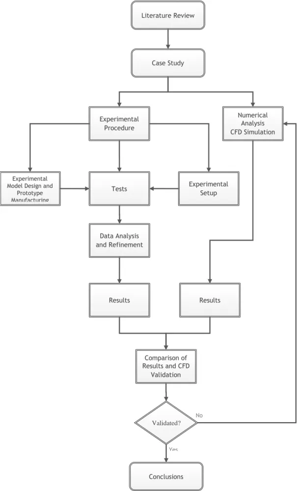
Figure 1.2 - Thesis structure flow diagram. ... 5

Figure 2.1 – Specifications of several HUGIN AUV’s [20]. ... 9

Figure 2.2 – ABE AUV during a mission (adapted from [1]). ... 10

Figure 2.3 – REMUS 6000 operating near free surface (adapted from [22]). ... 11

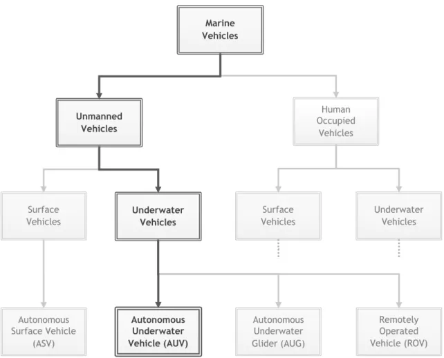
Figure 2.4 - Global classification of marine vehicles. ... 12

Figure 2.5 - Relationship between Endurance, Time, Range and Maneuverability (adapted from [4]). ... 13

Figure 2.6 – Resistance Force decomposition (adapted from [24]). ... 15

Figure 2.7 – Resistance force components for a streamlined body with constant volume in an infinite fluid domain at constant velocity (adapted from [25]). ... 18

Figure 2.8 - Axisymmetric hull shapes (adapted from [31]). ... 19

Figure 2.9 - Total resistance coefficient vs Submergence depth (adapted from [24]). ... 21

Figure 2.10 - According Moonesun et al., Milestone and fully submergence depth for all Froude numbers (adapted from [24]). ... 22

Figure 2.11 – Comparison of normal force coefficient (a); hydrodynamic center (b) and pitch moment (c) between towing tank results and Jorgensen results (adapted from [8]). ... 26

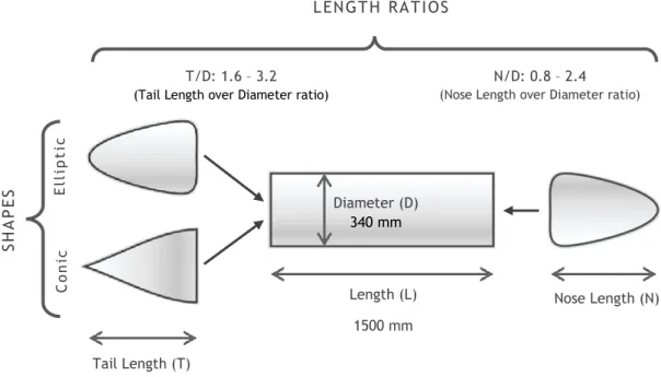
Figure 3.1 - Characteristics (dimensions, ratios and shapes) of all components of full-scale prototype used for this study. ... 30

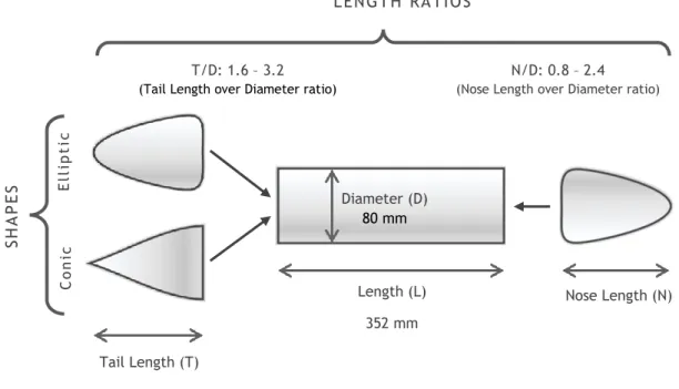
Figure 4.1 - Characteristics (dimensions, ratios and shapes) of all components of AUV model used for this study. ... 34

Figure 4.2 - Left image shows the body without nose and tail. Right image shows the body with an elliptical nose and tail. ... 35

Figure 4.3 - Experimental configuration. ... 35

Figure 4.4 - AoA system: left) 0 degrees; middle) 10 degrees; right) 20 degrees. ... 35

Figure 4.5 - Experimental manufactured components. ... 36

Figure 4.6 - Experimental laboratory layout. ... 37

Figure 4.7 - Full experimental design. ... 37

Figure 4.8 - Final metallic structure assembled before mounting at the towing tank. ... 39

Figure 4.9 - Final Experimental Setup. ... 39

Figure 4.10 – Procedure adopted to calculate the Drag caused, exclusively, by the hull body. ... 43

Figure 5.1 - Control Volume dimensions. ... 56

Figure 5.2 - Shape of the Wake for an improved Mesh treatment. ... 59

Figure 5.3 - Left) Mesh Result; Right) Detailed Nose Mesh Result. ... 60

Figure 5.4 - Velocity contours/vectors for different Tail configurations at nominal velocity (full-scale prototype) of 0.45 m/s. ... 65

Figure A.1 – Full Prototype Configuration after manufacturing; Here, it can be seen the hull body at 20˚ of AoA during testing stages. ... 75

Figure A.2 – Nose and Tail configurations; Here, it can be seen several Nose/Tail configurations used on Experimental Tests. ... 75

(14)

Figure B.1 – Towing tank without water; Here, it can be also seen a first unsuccessful mount configuration with a different motor. ... 77 Figure B.2 – Model’s attitude travelling at 20˚; Here, it can be seen the hull body at the starting position... 77 Figure C.1 – Initial Experimental Setup; As can be seen, a different motor and tube were also tested. ... 79 Figure C.2 – Initial Dynamometer used; Here, it can be also seen the tubes where the water entered on the Towing Tank. ... 79 Figure C.3 – System added to the Towing Tank for an autonomous returning. ... 80 Figure C.4 – Thread System used; the supporting blue thread was used to guarantee a safe distance between the pulling/pushing thread. ... 80 Figure C.5 – Experimental System used during Experiments; Several attempts/considerations were made to achieve this Setup. ... 81 Figure D.1 – Frequency Inverter used; Here, it can be seen a pre-programmed run for 13 Hz (0.75 m/s). ... 83 Figure D.2 – System used to measure the Towing Carriage Drag; Here, it can be seen an attached device to the Load Cell to communicate (wireless) with the Receiver Device. A safe system was made to guarantee material’s safety. ... 84 Figure D.3 – WiSTAR Device used to receive Data via Wireless. ... 84 Figure E.1 – Weights used for Experimental Tests (range of 50 to 3000 g). ... 85 Figure E.2 – Towing Carriage with Weights; Here, it can be seen that depending on hull’s AoA, the Weights position changes. ... 85

(15)

List of Tables

Table 2.1 - SPURV I Specifications (adapted from [18]). ... 8

Table 3.1 - Prototype’s Operation Envelope. ... 29

Table 4.1 – Towing tank dimensions. ... 31

Table 4.2 - Model’s parameters according full scale prototype (h considered since the body’s longitudinal centerline to water’s surface). ... 32

Table 4.3 - Model’s parameters according full scale prototype (h considered since the body’s surface to water’s surface). ... 32

Table 4.4 – Fluid and Towing tank properties. ... 36

Table 4.5 - Experimental conditions; *Elliptical shape; Elliptic and Conical shapes. ... 37

Table 4.6 - Nose characteristics with buoyancy. ... 41

Table 4.7 - Tail characteristics with buoyancy. ... 41

Table 4.8 - Mass Combinations. ... 41

Table 4.9 - Combinations weight with its adding load values. ... 42

Table 4.10 – Corresponding Velocity for each Frequency. Elliptic Nose 192mm – Elliptic Tail 256mm, distance 4.48m. ... 44

Table 5.1 - Several Meshing parameters tested. ... 58

Table 5.2 - Fluid properties. ... 60

Table 5.3 – Reynold’s Similarity applied. ... 62

Table 5.4 – Error % between Exp. & Num. Results (Elliptical & Conical Tails, respectively). .. 64

Table F.1 – Parameters considered for each case; Here, as can be seen, several parameters were calculated; For each case, 10 runs were made. However, these 10 runs are omitted here (only final values are shown). ... 87

Table F.2 – Data collected for one Drag value; Here, each column represents data collected for one run. After 10 runs, the average value and the standard deviation were calculated; consecutively, the undesired values were excluded through data refinement (using the average value and the standard deviation). ... 89

(16)

(17)

List of Charts

Chart 4.1 – Drag Results for different velocities operating at 0 degrees, varying N/D between 0.8 to 1.6, and fixing the T/D = 3.2. ... 46 Chart 4.2 - Drag Results for different velocities operating at 0 degrees, fixing N/D and varying T/D between 1.6 to 3.2. ... 46 Chart 4.3 - Drag Results for different AoA’s operating at 1 m/s, varying N/D between 0.8 to 1.6, and fixing the T/D = 3.2. ... 47 Chart 4.4 - Drag Results for different AoA’s operating at 1 m/s, fixing N/D and varying the T/D between 1.6 to 3.2. ... 48 Chart 4.5 - Drag Results for different velocities operating at 0 degrees, varying N/D between 0.8 to 2.4, and fixing the T/D = 3.2. ... 49 Chart 4.6 - Drag Results for different velocities operating at 0 degrees, fixing N/D and varying T/D between 1.6 to 3.2. ... 49 Chart 4.7 - Drag Results for different AoA’s operating at 1 m/s, varying N/D between 0.8 to 2.4, and fixing the T/D = 3.2. ... 50 Chart 4.8 - Drag Results for different AoA’s operating at 1 m/s, fixing N/D and varying T/D between 1.6 to 3.2 ... 51 Chart 4.9 - Comparison of Drag Results between Conical and Elliptical tail shapes, for

different AoA’s on a velocity of 1 m/s. FALTA LEGENDAR CORRECTAMENTE ... 52 Chart 4.10 - Comparison between Elliptical and Conical tail shapes, for different velocities at 0 degrees of AoA. ... 53 Chart 4.11 - The influence of AoA’s (0 - 20˚) on Drag, for different velocities (0.5 - 1.00 m/s). ... 54 Chart 4.12 - The influence of Velocity (0.5 – 1.00 m/s) on Drag, for different AoA’s (0 - 20˚). ... 54 Chart 5.1 - Mesh-independency study (referent to Table 5.1). ... 61 Chart 5.2 - Comparison of CD Results between Numerical and Experimental Procedure varying

T/D ratio between 1.6 to 3.2 for an Elliptical Tail shape case. ... 63 Chart 5.3 - Comparison of CD Results between Numerical and Experimental Procedure varying

(18)

(19)

List of Acronyms

ABE Autonomous Benthic Explorer AGAVE Artics GAkkel Vents Expedition AKN Abe-Nagano-Kondoh

AoA Angle of attack

ASE Analytical and Semi-Empirical ASV Autonomous Surface Vehicle ASW Anti-Submarine Warfare AUG Autonomous Underwater Glider AUSS Advanced Unmanned Search System AUV Autonomous Underwater Vehicle CAD Computer-Aided Design

CEiiA Centre of Engineering and Product Development CFD Computational Fluid Dynamics

CN3 Communications/Navigation Network Node CNC Computer Numeric Control

CV Control Volume

DNS Direct Numerical Simulation

EMEPC Estrutura de Missão para a Extensão da Plataforma Continental FFI Norwegian Defence Research Establishment

HOV Human Occupied Vehicle

IFREMER French Research Institute for Exploitation of the Sea IMAR Institute of Marine Research

IMPA, IP The Portuguese Sea and Atmosphere Institute, I.P. ISR Instituto de Sistemas e Robótica

IST Instituto Superior Técnico

ITTC International Towing Tank Conference LARS Launch And Recovery System

LES Large Eddy Simulation

MARINET Marine Renewables Infrastructure Networks MCM Mine CounterMeasures

MIG Metal Inert Gas

MIT Massachusetts Institute of Technology PC Personal Computer

PIV Particle Image Velocimetry RANS Reynolds Averaged Navier-Stokes REMUS Remote Environmental Monitoring UnitS RNG Renormalization-group

ROV Remotely Operated Vehicle RSM Reynolds Stress Model SLS Selective Laser Sintering

SPAWAR Space and Naval Warfare Systems Command SPURV Special Purpose Underwater Research Vehicle SST Shear-Stress Transport

(20)

USA United States of America

UUST Unmanned Untethered Submersible Technology UUV Unmanned Underwater Vehicle

WB WorkBench

WHOI Woods Hole Oceanographic Institution WWII Word War Two

(21)

Nomenclature

B Buoyancy [N]

Bl Blockage Ratio [-]

CD Drag coefficient [-]

CF Friction Resistance Coefficient [-] CP Prismatic Coefficient [-] CR Residual Drag Coefficient [-]

D Diameter [mm]

d Distance [m]

DT Drag [N]

Fn Froude Number [-]

FR Resistance Force [N]

g Acceleration due to Gravity [m/s2_]

h Submergence depth [mm]

H* _{Submergence depth-to-diameter Ratio} _[-] K Thermal conductivity coefficient [-]

L Length [mm]

l Characteristic Linear Dimension [m]

m Mass [g]

p Pressure [Pa]

q Fluid Velocity Vector [m/s]

Re Reynolds Number [-]

S Wetted Surface Area [m2_]

SO Maximum Cross Sectional area of the Towing Tank [m2]

t Time [s]

U Velocity [m/s]

V Volume [m3_]

Greek letters

y Distance of the first layer of the cells to the hull [mm] y+ _{Distance from body’s surface to the near wall node} _[-]

α Maximum Cross Sectional area of the Model [m2_]

γ Specific Heats Ratio [-] δij Kronecker delta function [-]

ε Turbulence Dissipation Rate [m2_/s3_]

κ Turbulence Kinetic Energy [m2_/s2_]

μ Absolute Viscosity [kg/(s.m)] μ* _{Friction velocity} _[m/s]

ν Kinematic Viscosity [kg/(s.m)]

ρ Density [kg/m3_]

τW Shear Stress [N/m2]

ω Specific Dissipation Rate [m2_/s3_]

(22)

(23)

Chapter 1

1 Introduction

1.1 Motivation

Oceans are a significant component of the Earth’s surface forming the majority of the hydrosphere. It is certain that the ocean covers more than 2/3 of the Earth’s surface, being a fundamental reason of human’s existence on Earth. Moreover, the average depth of the ocean is 3680 meters and the greatest ocean depth of the oceans is found in Mariana’s trench, with 10911 m depth. However, only about 5% of the oceans bottoms have been explored [1]. Therefore, it is extremely important to explore as much as possible this unknown area and understand how oceans can improve human lives. The collection of ocean data by observation and tracking in actual sea is crucial.

In order to understand the ocean, several tools have been used in the offshore industry since the late 1960s. These tools must comply with certain characteristics to carry out their functions [2]. Lately, tools as Human Occupied Vehicles (HOV’s), Remotely Operated Vehicles (ROV’s) and Autonomous Underwater Vehicles (AUV’s) are being used for an extensive and complex study of the oceans, revolutionizing the process of gathering ocean data [1], [3]. However, the relative high cost of using instruments lowered from research ships (HOV’s) or tethered robots (ROV’s) and their limitations such as the need for a communications tether or an operating vessel have limited their use. Consequently, AUV’s became a common tool in ocean sampling by being independent, and are now an indispensable feature for collecting ocean data providing a safe, cost-effective and reliable alternative to manned or remotely controlled systems [4]– [7].

In recent years, AUV’s are becoming a powerful tool in deep ocean research, being increasingly used in areas such as, the exploration of underwater environments, maintenance and repair of submerged structures, mineral exploration, military use, pipeline inspection, mine-sweeping and many other areas [8], [9]. These several distinct applications give rise to a large number of different vehicle shapes and sizes. The design of AUV’s is conducted by a demanding tradeoff between the crucial requirements of the missions, and the main constraints of fabrication, assembly and operational logistics. However, an AUV is limited when power requirements are concerned, which directly impacts its characteristics, such as velocity, range and endurance of the vehicle [6], [10]. Thus, it is crucial to find an efficient hydrodynamic design that reduce power consumption, and in turn, increase AUV’s autonomy. In order to improve its performance on a design project level, the reduction of hull’s hydrodynamic resistance must be the main

(24)

Research Objectives and Aim Chapter 1 • Introduction

focus. Therefore, an increasing use of AUV’s leads the need to investigate and predict, efficiently, the hydrodynamic forces acting over an AUV [11].

This research thesis further analyzes, through the use of experimental and numerical methods, the hydrodynamic forces and coefficients of an AUV with a torpedo shape operating under deeply submerged conditions. The AUV model velocity, Angle of Attack (AoA), Nose Length / Diameter and Tail Length / Diameter ratios are investigated to study their effect on hydrodynamics performance of submerged vehicles. For this purpose, a detailed experimental procedure has to be performed by a numerical study using a commercial Computational Fluid Dynamics (CFD) tool, FLUENT ANSYS 16.0., being the ultimate goal of this thesis the validation of the numerical simulation against the experimental procedure, allowing for the optimization of the overall AUV body.

1.2 Research Objectives and Aim

CEiia - the Centre of Engineering and Product Development challenged the author of this thesis to study, experimentally and numerically, the hydrodynamic forces and coefficients of an AUV model based on MEDUSA DEEP-SEA AUV type. MEDUSA Deep-Sea AUV is a double-hull design that is currently being developed by a group of partners: CEiiA, Instituto de Sistemas e Robótica (ISR) from Instituto Superior Técnico (IST), The Portuguese Sea and Atmosphere Institute, I.P. (IPMA, IP), EMEPC (Estrutura de Missão para a Extensão da Plataforma Continental) (governmental structure with a mission to prepare/monitor the process of extending the continental shelf of Portugal), Institute of Marine Research (IMAR) and Argus Remote Systems AS. This project embraces the design and production of a specific AUV for the required conditions imposed initially to operate at 3000 m of depth and with a specific payload. More details about this project are shown in reference [12]. Vehicle’s configuration is shown in Figure 1.1. This thesis is not a part of MEDUSA Deep-Sea project, being rather considered a parallel study which might help optimize this vehicle’s hydrodynamic hull efficiency.

(25)

The following objectives were defined for this research:

- Investigate the effects of velocity, AoA, Nose/Diameter and Tail/Diameter ratios on the hydrodynamic forces and coefficients generated by an AUV hull form operating in a fully submerged depth condition;

- Implement the experimental procedure to investigate the hydrodynamic forces and coefficients;

- Investigate the application of CFD numerical methods for predicting underwater vehicle’s hydrodynamic coefficients;

- Validate the numerical simulation process against the experimental testing results; - Identify optimum configurations and conditions for AUV’s taking into consideration

vehicle’s velocity, AoA, Nose/Diameter and Tail/Diameter ratios.

The aim of this project is to validate the numerical simulation against the experimental procedure (see Figure 1.2). For this purpose, the towing tank of UBI shall be set properly to do the experiments and experimental data should be collected. The CFD tool shall be used to obtain numerical data to achieve the proposed objectives.

1.3 Research Strategy and Document Structure

The research strategy undertaken in this project comprises the use of the following three interrelated research tools:

- Investigation through an extensive literature review to report on the relevant work completed by other authors, and support the experiment and numerical based investigations;

- Investigation by experiment to observe, measure and register the hydrodynamic forces and calculate coefficients through data collected, of a fully submerged AUV hull form;

- Investigate, implement, analyze and evaluate a CFD numerical simulation to predict the resistance force and drag coefficient experienced by a fully submerged AUV model.

This document is structured in a coherent and logical manner. The description of each chapter within this document is presented below:

Chapter 1 introduces the motivation to the research problem, presents its aim and the research objectives expected to be achieved during this study.

Chapter 2 provides a literature review of Unmanned Underwater Vehicles (UUV’s), the hydrodynamic phenomena environment of a submerged AUV body and the relevant experimental and numerical research completed to date by other authors.

(26)

Research Strategy and Document Structure Chapter 1 • Introduction

Chapter 3 describes the specific case study of this thesis, as well as its requirements and parameters that are aimed to be studied.

Chapter 4 presents the experimental procedure, including the experimental model design and its manufacturing, and experimental setup, used to calculate the forces of the AUV model operating without free surface and wall effect. It also presents the results of the experimental tests.

Chapter 5 discusses the CFD software used to simulate and predict the hydrodynamic forces and coefficients of the AUV model, assuming fully submerged depth condition. It also provides the modelling and simulation methods adopted in this research, as well as its results.

Chapter 6 presents the conclusions drawn from the experimental procedure and numerical simulation, the difficulties encountered during this thesis, and the areas which need further investigation.

(27)

Figure 1.2 - Thesis structure flow diagram. Literature Review Case Study Conclusions Validated? Yes No

(28)

(29)

Chapter 2

2 Literature Review and Significant Theory

It is essential to understand background knowledge and fundamental milestones about the AUV history, as well as, similar studies made by other authors. It is also important to understand the reasons for the underwater vehicle’s shape at different phases of their development and some notable achievements.

2.1 History

AUV’s are directly linked to streamlined bodies, being the majority torpedo-shaped. The first torpedo was invented by Robert Whitehead in Austria in 1866 [13], [14], but this concept only started being dominant and reliable since World War II (WWII) [15]. The name Torpedo came from the Torpedo fish, which is an electric ray capable of delivering a stunning shock to its prey. The torpedo can be considered the first AUV, if the fact that it carried an explosive payload is ignored. Furthermore, this torpedo achieved a speed of 3 m/s and ran around 700 m [16]. The torpedo-shaped is a crucial parameter for this study because it is straightly connected with actual AUV’s design.

The development of UUV’s started in the 1960’s and some initial research was made about the utility of UUV’s. The first successful one was developed as early as 1957 in the Applied Physics Laboratory at the University of Washington to gather data from the Arctic regions. This UUV was named as the Special Purpose Underwater Research Vehicle (SPURV I) and was subject of study until the mid 70’s. Between the 70’s and 80’s the SPURV II was adopted, an upgrade more capable than SPURV I. Altogether were released over 400 SPURV [16], [17]. Table 2.1 shows some of SPURV I’s specifications.

(30)

History Chapter 2 • Literature Review and Significant Theory

Table 2.1 - SPURV I Specifications (adapted from [18]).

Maximum Depth 3600 [m]

Endurance with LR 90 battery 5.5 hours (hr)

Instrument Payload 45 [kg]

Speed 2-2.5 [m/s]

Displacement (sea water) 430 [kg]

Net Buoyancy 9.1 [kg] Overall Length 3.1 [m] Diameter 0.508 [m] Dive Rate 1.3 [m/s] Climb Rate 2.3 [m/s] Turn Rate 3 [˚/s]

Acoustic Tracking Range 2000 [m]

In 1973, the Naval Ocean System Center, now known as Space and Naval Warfare Systems Command (SPAWAR) started to develop the Advanced Unmanned Search System (AUSS). This vehicle was ready for the first launch ten years later, in 1983. Had a displacement of 907 kg, with 5,2 m long and 0,8 m of diameter, completed over 114 dives being some of them to 6000 m of depth [5], [16].

In 1976, the French Research Institute for Exploitation of the Sea (IFREMER) designed Epulard vehicle. This vehicle was assembled by 1978 and was operational for the first dive in 1980. It had a maximum depth of 6000 m and was acoustically controlled, Epulard completed about 300 dives between 1970 and 1990 [16].

During the 70’s, other AUV’s were also developed at the Massachusetts Institute of Technology (MIT). Later, in 1997, a group of engineers from the MIT AUV Laboratory founded BLUEFIN ROBOTICS. This company develops, builds, and operates AUV’s and related technologies. Recently, was acquired by General Dynamics Mission Systems, a business unit of General Dynamics [19].

In 1980, the “International Symposium on Unmanned Untethered Submersible Technology” (UUST) was created in Durham, New Hampshire, United States of America (USA), with twenty-four technologist attending this conference. Seven years later, more than 320 people were representing more than 100 companies, 20 Universities and 20 federal agencies on the meeting [17].

(31)

During the 80’s, there were many technological advances apart from AUV community that critically improved AUV development. Improvements like software systems and size reduction of hardware systems were crucial. Following Busby’s 1987 Undersea Vehicle Directory, there were six operational AUV’s and other 15 vehicles considered prototypes or under construction by 1987 [5], [16].

In 1990, the HUGIN AUV program started in a project between KONGSBERG and the Norwegian Defence Research Establishment (FFI). Since its development has been the most capable and successful commercial AUV in operation. Figure 2.1 shows the HUGIN AUV Product Range and their specifications [20], [21].

Figure 2.1 – Specifications of several HUGIN AUV’s [20].

In the 90’s, the first generation of operational systems able to be tasked to perform defined objectives appeared, in other words, AUV’s grew from proof of concept to a final result. Therewith, the interest in AUV’s academic research increased quickly.

During the 90’s, the Massachusetts Institute of Technology’s Sea Grand AUV lab developed six Odyssey vehicles. These vehicles had a displacement of 160 kg, with an operational speed of

(32)

History Chapter 2 • Literature Review and Significant Theory

1.5 m/s, operating for up to six hours and were assigned to 6000 m of depth. In 1994, these vehicles operated under ice, and in 1995 operated for 3 hours in the open ocean to a depth of 1400 m [16], [17].

Almost at the same time, in the early 90’s, the Woods Hole Oceanographic Institute (WHOI) developed the Autonomous Benthic Explorer (ABE) (see Figure 2.2). ABE completed its first scientific mission in 1994, had a displacement of 680 kg and its dives typically lasted about 16 to 34 hours depending on the instrument payload and bottom terrain. This vehicle was the first one to be completely independent of the surface vessel and capable of covering large areas of underwater terrain. ABE was extremely maneuverable due to its six thrusters. Its deepest dive to date was 4000 m, in its at least 80 dives [5], [16]. Figure 2.2 demonstrates ABE AUV attached to the Launch And Recovering System (LARS).

Figure 2.2 – ABE AUV during a mission (adapted from [1]).

At the same time, the South Hampton Oceanography Center’s AUTOSUB was developed. AUTOSUB was the first vehicle prepared for long duration missions, having completed its first scientific mission in 1998. With a travelling speed of 1.5 m/s, it displaces 1700 kg and can operate for up to six days. This vehicle has completed over 270 missions covering more than 3500 km. Its longest mission lasted 50 hours [5], [16].

In the late 90’s, WHOI’s Remote Environmental Monitoring UnitS (REMUS) vehicle was developed in the Oceanographic Systems Lab (now marketed by Hydroid, owned by Kongsberg Group in 2007) to support scientific objectives at the LEO-15 observatory in Tuckerton, New Jersey. Its first scientific mission was in 1997 and there are currently over 50 REMUS vehicles in 20 different configurations that are being independently operated by universities and agencies, so

(33)

Its longest mission lasted 17 hours, with an operational speed of 1.75 m/s at a maximum depth of 20 m of the coast of New Jersey [1], [16]. The Figure 2.3 shows a recent version of a REMUS AUV, the REMUS 6000. This vehicle can operate in water depths up to 6000 m and its autonomy depend on its speed/sensor configuration (typical mission duration is 22 hr).

Figure 2.3 – REMUS 6000 operating near free surface (adapted from [22]).

In 1997, the HUGIN I AUV made the first commercial survey operation for the Ásgard Gas Transport Pipeline Route. This is an important milestone for the AUV civilian application. This survey confirmed the expected improvements in efficiency and data quality by the use of AUV’s. From 2001, these vehicles have been successfully used for military application [20].

In 2004 the Navy UUV Master Plan was issued. This plan defines UUV missions in the following prioritized order [23]:

1. Intelligence, Surveillance, and Reconnaissance; 2. Mine Countermeasures (MCM);

3. Anti-Submarine Warfare (ASW); 4. Inspection/Identification; 5. Oceanography;

6. Communications/Navigation Network Node (CN3); 7. Payload Delivery.

This UUV Master Plan is a document recommending AUV missions and technologies.

Since the beginning of this century, it became clear that the use of AUV technology was of great value for several commercial tasks. There is a transitioning point in which AUV technology will definitely move from the research environment into the commercial offshore industry. Although, there are some parameters to be performed, such as the economic viability of the

(34)

Unmanned Underwater Vehicles (UUV’s) Chapter 2 • Literature Review and Significant Theory

technology and some technological problems, to continue its advance for industry to embrace its potential.

Currently, there are many companies on the AUV industry such as Kongsberg Maritime (owner of the most-known brands as REMUS, HUGIN, MUNIN or SEAGLIDER), BLUEFIN ROBOTICS or International Submarine Engineering. These companies are being constantly supported by research institutions as WHOI, MIT AUV Laboratory or Kongsberg Group (two centuries business company, owner of Kongsberg Maritime) to expand this industry.

2.2 Unmanned Underwater Vehicles (UUV’s)

Since the main topic of this thesis is AUV’s, it is not relevant to have an exhaustive study about all marine vehicles. However, it is extremely important to understand their global classification like it is shown in Figure 2.4.

Figure 2.4 - Global classification of marine vehicles.

Unmanned Vehicles can be described by dividing them into two categories: Underwater Vehicles and Surface Vehicles.

(35)

The Unmanned Surface Vehicles, most known as Autonomous Surface Vehicles (ASV’s) are vehicles that only operate in the ocean’s surface. Depending on its vessel, length and power supply, they can operate for a considerable time (weeks or months).

The Unmanned Underwater Vehicles (UUV’s) are mainly separated into three categories: Remotely Operated Vehicle (ROV), Autonomous Underwater Vehicle (AUV) and Autonomous Underwater Glider (AUG). Depending on each specific task, the type of UUV should be chosen properly. However, characteristics such as high endurance, long operation time, high maneuverability and range are always desired. The relationships between those four characteristics are shown in Figure 2.5.

Figure 2.5 - Relationship between Endurance, Time, Range and Maneuverability (adapted from [4]).

2.3 Autonomous Underwater Vehicles – Design and Concepts

The design of an AUV depends on its mission and in a preliminary design concept it is highly important to understand which geometry/shape is better for the desired mission.

Nowadays, with the development of technology came the increase in the use of AUV’s. Mainly, there are three different types of applications for AUV’s:

- Commercial: directly linked with oil and gas industries; its traditional missions are the mapping and tracking of the seafloor before construct any infrastructure, also pipelines can be monitored easily.

- Defense: obviously connected with defense or protection; this AUV application involve missions as mine detection, monitoring an area to identify unknown objects and detection of manned submarines (anti-submarine warfare).

- Research: this is the pioneer application, came with the necessity to know the ocean’s life and study precisely new elements attached to the sea floor.

Depending on each mission, there are several variables that can be changed during the preliminary design such as, for example, the AUV Length (L) and/or Diameter (D).

(36)

General Design of an AUV Chapter 2 • Literature Review and Significant Theory

2.4 General Design of an AUV

There are some aspects in AUV design that need special attention, and are known as major design aspects. These aspects include: hull design, propulsion, submerging and electric power [2]. Therefore, these aspects can be subdivided into several subsystems as [23]:

- the pressure container; - the hydrodynamic hull; - ballasting;

- power and energy;

- electrical-power distribution; - propulsion;

- navigation and positioning; - obstacle avoidance; - masts;

- maneuver control; - communications;

- locator and emergency equipment; - payloads.

Since the aim of this thesis is to estimate/calculate the hydrodynamic forces/coefficients, it is crucial to improve backgrounds in hull design, and specifically in hydrodynamic hull. For a detailed study about the subsystems please refer to the references [2], [23].

2.4.1 Hydrodynamic Design

An AUV when travelling through the ocean should be highly hydrodynamic or as much as possible streamlined. Frequently, the components housing defines several restrictions as minimum Diameter (cross-sectional area) or Length, and these restrictions directly affect the body’s hydrodynamic. Reduce Drag (DT), or also known as Resistance Force (𝐹𝑅), is always one of the

main design objectives. Moreover, the flow over an AUV’s body should be controlled for an efficient propulsion i.e. laminar flow designs should be chosen [23]. Maximum cross section from nose and nose/tail radius (same length with different curvature) are parameters that also have influence on resistance force, but since they are not controllable due to the constraints of this study, will be neglected. The FR depends on a set of phenomena as can be shown in

(37)

Figure 2.6 – Resistance Force decomposition (adapted from [24]). This resistance force is represented by the relationship presented in Equation (2.1)

𝐹𝑅=

1

2. 𝜌 . 𝐶𝐷 . 𝑈2 . 𝑆 (2.1) Where 𝜌 is density, 𝐶𝐷 the Drag coefficient, U is the model velocity and 𝑆 the wetted surface

area.

Following the equation above, the Drag coefficient is given by the Equation (2.2),

𝐶𝐷=

𝐹𝑅

(38)

Where all parameters are known from the Equation (2.1). The author considered relevant to describe these two similar equations, since these are fundamental for this study.

Generally, the resistance force can be divided into three different components: form drag or pressure drag (also known as viscous pressure resistance), friction resistance and wave resistance. Since this study is for a fully submerged mode i.e. there is no free surface effect. Knowing that the main difference between submerged mode and surfaced mode is wave-breaking and wave-making, the wave resistance is neglected in the scope of this study. To understand the influence of free surface effect (two-phase flow condition) see E. Dawson [25]. Henceforth, a fully submerged condition is always assumed by the author. Therefore, there are two dominant factors responsible by the submerged body’s resistance to motion when moving in a homogenous viscous fluid domain: friction resistance (tangential shear forces) and viscous pressure resistance (normal pressure forces) resistance, as marked in Figure 2.6.

The friction resistance coefficient is given by the Equation (2.3):

𝐶𝐹=

0.075 (log10𝑅𝑒 − 2)2

(2.3) Where 𝐶𝐹 is the non-dimensional frictional resistance coefficient and 𝑅𝑒 is the Reynolds

number. Knowing 𝐶𝐹 and 𝐶𝐷(given in Equation (2.2)) the Residual Drag coefficient (𝐶𝑅) can be

obtained from the Equation (2.4):

𝐶𝑅= 𝐶𝐷− 𝐶𝐹 (2.4)

The residual drag is a significant parameter for hydrodynamic studies defined as total resistance except for skin friction drag.

The influence of each component on resistance force is dependent on the size and shape of the body, as shown in Figure 2.7. There is no precise minimum in total drag but various authors refer an optimum L/D ratio for a streamlined body is between 6 and 7. This optimum value changes depending on its shape. In order to reduce the form resistance, the hull length can be extended. However, the resultant increase in length and wetted surface area leads to an increase in friction resistance. Then, the effects of L/D ratio on the two components are contradictory, where the lowest point of total resistance force is related to the optimum L/D ratio, as shown in Figure 2.7.

Reynolds number (𝑅𝑒), mentioned in Equation (2.3), is an essential parameter used on this thesis for dynamic similarity between the full-scale AUV prototype and hull model used for this study. To assume similar flow conditions, applied on this case, the Reynolds number needs to be the same for both scales i.e. Reynold’s law must be ensured (the inertial and frictional

(39)

only valid when fluid properties of both scales are the same. Due to Reynolds number appears in RANS equations, it has an effect on all flows governed by these equations. Reynolds Number (hereinafter, Reynolds Number is going to referred as Re) is defined by the ratio of the fluid’s inertia forces to the viscous forces in the boundary layer of the fluid and it is given by the Equation (2.5),

𝑅𝑒 = 𝑈. 𝑙_𝜇

𝜌 (2.5)

Where μ is absolute viscosity and 𝑙 the characteristic linear dimension. The denominator is also known as (Equation (2.6)),

𝜈 = 𝜇

𝜌 (2.6)

Consecutively, the Reynold’s similarity is represented by the Equations (2.7) and (2.8), (𝑅𝑒)𝑀= (𝑅𝑒)𝑃 (2.7)

𝑈𝑀= 𝑈𝑃. (

𝐿𝑃

𝐿𝑀)

(2.8) Where the subscript M represents Model and P the full-scale Prototype.

Since 𝑅𝑒 appears in several applications, 𝑙 represents one of many length scales. The transition point (point which the boundary layer changes from laminar to turbulent) is dependent of 𝑅𝑒 i.e. as Re increases, this point moves forward on the surface [26]–[29].

Another parameter which influences resistance of the streamlined body is the prismatic coefficient (𝐶𝑝), that describes the amount of volume on the ends of the body. It is formed as

“the ratio of the displaced volume with that contained in a prism formed by the mid-ship cross-sectional area and the length”[30]. An optimum 𝐶𝑝 value is around 0.6 [25], [31]. The 𝐶𝑝 is

defined as (Equation (2.9)): 𝐶𝑝= 𝛻 𝜋 4 . 𝐷2 . 𝐿 (2.9) Where 𝛻 is the volume of the envelope, 𝐷 the maximum hull diameter and 𝐿 the body’s length. According to Joubert [30], reducing both L/D ratio and 𝐶𝑝 “should give a reduction in total

(40)

Figure 2.7 – Resistance force components for a streamlined body with constant volume in an infinite fluid domain at constant velocity (adapted from [25]).

The viscous pressure drag varies along the body’s surface, being its biggest value at the nose (called stagnation point), where the streamlines divide through the body. The pressure is smaller when the streamlines are straight, and rises when are diverging. In an ideal fluid (fluid with no viscosity), the nose and tail pressure would be the same i.e. the integral of all pressures acting on the body’s surface would be zero [25], [31].

However, in a real fluid, the viscosity is an important property that causes tangential force or friction resistance. This phenomenon occurs due to the interaction between the fluid and the body, and the formation of a fluid boundary layer around the body’s surface. The boundary layer depends on the relative velocity, location along the body’s length and the effects of local pressure gradients. The flow along the boundary layer can be either laminar or turbulent with a transitional region dividing the two [25], [31]. A detailed description of boundary layer is presented by [32], [33].

2.4.2 Hull Shape

According to the given backgrounds above, it is extremely important to choose the most efficient hull shape in order to get the lowest drag possible.

Mainly, two types of axisymmetric bodies were considered, these seem to be admitted by all authors with similar studies [8], [24], [34], [35]. These bodies are shown in Figure 2.8. A round hull presents no stress concentrations and when compared to other shapes is able to withstand more pressure, except for the spherical form. The spherical form is not considered on this study, even though being the most effective hydrodynamic shape. There are some aspects as strength, maneuverability, form resistance (L/D ratio = 1), propulsive efficiency or power

(41)

Figure 2.8 - Axisymmetric hull shapes (adapted from [31]).

On Figure 2.8 (a) the shape presented is, known as the teardrop shape, this is the most ideal shape for submerged mode. Although, due to several issues on its construction and power housing requirements, the most conventional and applied form on AUV’s is the parallel mid-body form (Figure 2.8 (b)). The nose and tail form, can be elliptical, conical or even parabolic.

2.4.3 Restrictions to the flow around the model

Depending on the model’s and tank size, there are some differences when an AUV model is towed in a towing tank or in the unrestricted water. These differences are usually referred to as the boundary effects. It may be classified into Wall Effect, Free surface effect and Blockage Effect [37].

The blockage ratio is defined as “the ratio of the maximum cross sectional area of the model to that of the towing tank.” [37]. Following this definition, the Blockage ratio is given by the Equation (2.10),

𝐵𝑙 = 𝑎

𝑆𝑂 (2.10)

Where 𝑎 is the maximum cross sectional area of the model and 𝑆𝑂 the maximum cross sectional

area of the towing tank.

Wall Effect only depends on tank’s width. A combination of limited width and depth is known as the Blockage Effect. This phenomenon is rather complex due to the interference of the tank sides and bottom i.e. model size has to be sufficiently small to avoid inherent hydrodynamic interference, and this is called reflected wave interference effects. Unfortunately, a model too small leads to additional inaccuracies on the quality of results obtained due to the similarity between the full scale prototype and the model test [37]. As a result, the largest model with

(42)

minimum interference induced must be found. During the last years, the International Towing Tank Conference (ITTC) [38] made a recommendation for finding a blockage correction, although there is a lack of literature available. The blockage ratio is the most important parameter of the blockage effect. Marine Renewables Infrastructure Networks (MARINET) [39] refer blockage ratio above 0.1 can introduce questionable results, whereas H.Kim and J.Moss [37] present a lower limit of blockage ratio below which the blockage effect has normally been considered to be insignificant is 0.006. However, MARINET also refer cases which wave making is small, could be used larger models with the appropriate correction for the remaining blockage effect [37], [39], [40].

As described previously, AUV’s have two modes of navigation: surfaced mode and submerged mode. In surface mode, the wave resistance (divided into two components: wave breaking and wave making) is a main part of resistance (up to 50%) of total resistance. Although, this thesis is only based on the submerged mode, however, to travel under water, it is important to know at which depth is the interference of free surface negligible i.e. the wave resistance is minimum and can be neglected [24], [35]. There are several studies to find this fully submerged condition.

Hoerner and Weinblum et al. [25] concluded that for submergence depth-to-diameter ratios of at least 5 (H* = 5.00) the wave resistance could be neglected, where H* is defined as (Equation (2.11),

𝐻∗₌ℎ

𝐷 (2.11)

Being ℎ the submergence depth of an axisymmetric body’s longitudinal centerline below the still waterline and 𝐷 the maximum diameter.

There are other authors that connected the fully submerged depth with maximum diameter or length of submersible hull. According to Moonesun et al. [24] several authors used different submerged depths for their studies as, ℎ = 𝐿/2, ℎ = 3𝐷 or ℎ = 5𝐷. Figure 2.9 shows the effect of the submergence depth on Drag Coefficient.

(43)

Figure 2.9 - Total resistance coefficient vs Submergence depth (adapted from [24]). Moreover, Moonesun et al. [24] compares this submergence depth with Froude number (𝐹𝑛) and concludes that it is an important parameter in the evaluation of submergence depth. Also concludes that exists one “Milestone depth” where wave resistance decreases more than 80% and other where there is no wave resistance called “Fully submerged depth”, as shown by the references above and as can be seen in Figure 2.10. Further, this author refers the “fully submerged depth for high Froude numbers is equal to 4.5D.” and the “milestone depth for high Froude numbers is equal to 0.125L.”. Moonesun et al. [24] presented the Froude number as a crucial parameter to study submergence depth, showing that for 𝐹𝑛 < 0.5 were considered ordinary values and for 𝐹𝑛 > 0.7 high values. These statements are supported by Figure 2.10. The Froude number appears in two-phase flow conditions (problems involving pressure boundary conditions) and it is only important for determining which depth there is no wave resistance. Since this thesis focus on one-phase flow condition, Froude number is only helpful to comprehend which depth is the fully submerged condition i.e. this means that if there is no free surface, this parameter is insignificant, as well as Weber and cavitation number (insignificant numbers for this thesis) [26], [28]. 𝐹𝑛 is given by the Equation (2.12).

𝐹𝑛 = 𝑈

√𝑔𝐿 (2.12)

(44)

Fluid Mechanics Foundations Chapter 2 • Literature Review and Significant Theory

Figure 2.10 - According Moonesun et al., Milestone and fully submergence depth for all Froude numbers (adapted from [24]).

2.5 Fluid Mechanics Foundations

Before examining the methods of Computational Fluid Dynamics, a review of the governing equations of fluid mechanics must be done.

The fluid is defined by the ratio of specific heats (γ), viscosity (μ) and the coefficient of heat conduction (κ). The motion of the fluid is controlled by governing equations and boundary conditions. Based on conservation laws, the governing equations of fluid mechanics are given by:

- Mass conservation equation or continuity equation (mass can be neither created nor destroyed);

- Momentum conservation equation (Newton’s 2nd_Law);

- Energy conservation equation (based on the 1st_{law of Thermodynamics).}

All details of these equations (considerations and forms) are fully described at references [41], [42]. Hence, only the final equations will be demonstrated.

The conservation of mass can be described as the net outflow of mass through the surface surrounding the volume has to equal to the time rate of decrease of mass inside control volume. The differential form of continuity equation (vector form) is given by the Equation (2.13):

𝐷𝜌

𝑑𝑡+ 𝜌 . (∇ . 𝑞 ) = 0 (2.13) Where 𝑡 is the time, 𝑞 is fluid velocity vector (μ, ν, w) and 𝐷 = 𝛿 + 𝑞 . ∇ is the material

(45)

The momentum conservation equation, based on Newton’s 2nd_{law of motion, is represented by}

the Equation (2.14), which represents the net force action on a system has to be equal to the time rate of change of momentum of system.

𝜌𝐷𝑞𝑖

𝐷𝑡 = 𝜌𝑓𝑖+ 𝛿𝜏𝑖𝑗

𝛿𝑥𝑗 (2.14)

Where 𝑓𝑖 is the component of the mass force per unit mass second in the 𝑖 direction, 𝜏𝑖𝑗 are the

stress components, and 𝑖, 𝑗 = (1,2,3), i.e. a matrix 3x3 of stress components. Assuming a Newtonian fluid (where the stress components are linear to the derivatives), a relation between velocity filed and stress components can be made, as shown in Equation (2.15) [44].

𝜏𝑖𝑗 = (−𝑝 − 2 3𝜇 𝛿𝑞𝑘 𝛿𝑥𝑘) 𝛿𝑖𝑗+ 𝜇 ( 𝛿𝑞𝑖 𝛿𝑥𝑗+ 𝛿𝑞𝑗 𝛿𝑥𝑖) (2.15) Where 𝜇 is the viscosity coefficient, 𝛿𝑖𝑗 is the Kronecker delta function, 𝑝 is the pressure and 𝑘

a dummy variable summed from 1 to 3. Replacing the stress components of Equation (2.15) into the Equation (2.14), the Navier-Stokes equations are achieved, as demonstrated in Equation (2.16). 𝜌 (𝛿𝑞𝑖 𝛿𝑡 + 𝑞 . ∇𝑞𝑖) = 𝜌𝑓𝑖− 𝛿 𝛿𝑥𝑖(𝑝 + 2 3𝜇∇ . 𝑞) + 𝛿 𝛿𝑥𝑗𝜇 ( 𝛿𝑞𝑖 𝛿𝑥𝑗+ 𝛿𝑞𝑗 𝛿𝑥𝑖) (2.16) Finally, to complete the system of equations comes the energy conservation equation, which states the 1st_{Law of Thermodynamics: “The sum of the work and heat added to a system will}

equal the increase of energy.”[45]. There are several forms of this equation in literature, the Equation (2.17) is one of these forms.

𝐷𝜌(𝑒 +1_{2 𝑉}2₎

𝐷𝑡 = ∇. (𝐾∇𝑇) − 𝑑𝑖𝑣w

(2.17) Where 𝐾 is the coefficient of thermal conductivity, 𝑒 is the internal energy per unit mass, 𝑇 is the temperature gradient, w is the vector of work associated with each control volume face and −𝑑𝑖𝑣w = 𝑊̇ the work done on the system [46].

2.6 Computational Fluid Dynamics (CFD) – Numerical Approach

The behavior of viscous fluid flow is described by Navier-Stokes Equations (Equation (2.16)). Fluid flow, in of the majority of the cases, is turbulent. Turbulent flows have as particular characteristic: transportation of quantities, as momentum, energy, and species concentration, with fluctuation (hardest case to solve, small scale and high frequency) [47], [48]. These complex equations need to be solved numerically by the use of computational methods, except for very simple cases. All of these computational, theoretical and numerical methods are known as Computational Fluid Dynamics.

(46)

Turbulence models Chapter 2 • Literature Review and Significant Theory

The computational fluid mechanics techniques use the Eulerian approach to solve all applications. However, Navier-Stokes equations varies with time, which denotes that is required averaging multiple solutions at a set of time steps [49]. This leads to a decomposition of Navier-Stokes equation into the Reynolds Averaged Navier-Stokes (RANS) equations. Furthermore, RANS equations introduces to a several unknowns (Reynolds stress) that requires a turbulence model to generate a closed system of solvable equations, i.e. turbulence model is used to close the system of mean flow equations [49].

RANS equations are the most widely used approach, although there are other approaches that can simulate with higher precision, as Large Eddy Simulation (LES) or Direct Numerical Simulation (DNS). LES solves the spatially averaged RANS equations, directly resolving larger eddies, but modelling small ones. However, due to the computational requirements it is not a feasible option. DNS solves the full RANS equations, simulating with accuracy all turbulent flows (all eddies included) without requiring turbulence models. However, this approach is not practical for engineering purposes, due to extremely high costs and computational resources required [50]. A more detailed study about this topic can be made by checking of references [29], [31], [42], [51] .

2.7 Turbulence models

Since this study comprises the use of a well-known commercial software called ANSYS FLUENT, it will be described the turbulence models related to this tool.

Therefore, the turbulent models provided by ANSYS FLUENT are: - Spalart-Allmaras model (one-equation model); - κ-ε models (two-equation model)

- Standard κ-ε model;

o Renormalization-group (RNG) κ-ε model; o Realizable κ-ε model.

- κ-ω models (two-equation model) o Standard κ-ω model;

o Shear-stress transport (SST) κ-ω model.

- Reynolds Stress Model (RSM) (seven-equation model); - Large Eddy Simulation (LES) model.

It is important to understand “that no single turbulence model is universally accepted as being superior for all classes of problems” [50]. So, depending on purpose/necessity and computational resources/time efficiency the choice of turbulence model should be made.

(47)

2.7.1 Standard κ-ε model

This is the most used turbulence model in engineering for industrial applications. It is known as being robust, economic and with a satisfactory accuracy for turbulent flows. As referred above this is a two-equation model, which allows to calculate the turbulent length and time scale by solving two transport equations. These equations are for turbulence kinetic energy (κ) and dissipation rate (ε). A limitation of this turbulent model is that it is only valid for fully turbulent flows. Further, at near-wall regions, wall functions must be used, due to ε equation. Although, several improvements were implemented on Standard κ-ε model, resulting in examples as κ-ε RNG model or κ-ε Realizable model, but as referred previously, a trade-off of purpose/computational resources should be made before choosing a turbulent model [48].

2.7.2 κ-ω SST model

This turbulence model is considered an “upgrade” of Standard κ-ω. Furthermore, it was developed to have the benefits of κ-ω model (near-wall region) and κ-ε model (freestream independence in the far field). The ω equation integrates a damped cross-diffusion derivative term. The consideration of the transport effects of the principal turbulent shear stress led to a modified turbulent viscosity formulation [42], [50].

2.8 Similar studies

Mansoorzadeh and Javanmard [52] presented the free surface effect on drag and lift coefficients of an AUV by comparing two-phase flow numerical simulation with single phase flow simulation and the experimental procedure. The study was performed at several submergence depths for 1.5 and 2.5 m/s. The study demonstrated that, for both AUV speeds, the influence of free surface on drag coefficient was decreasing as the model distance from the free surface was increasing. A maximum difference of 10% between the numerical and experimental results for drag coefficient was observed. These authors concluded that it is not very straightforward to compare which method is more accurate, since there are errors and uncertainties associated with each one. Although, collecting data from both methods and compare them seemed to conclude better results.

J.L.D. Dantas and E.A. de Barros [11] investigated the hydrodynamic forces and coefficients obtained by an AUV with control surface deflection and angle of attack by the use of CFD software based on the Reynolds-Averaged Navier-Stokes (RANS) equations. These authors conducted their CFD simulations separately (AUV bare hull and control surface), to better predict each interference and compare with experimental results obtained in a towing tank. They concluded that the k-ω SST turbulent model was the best model to predict hydrodynamic coefficients and the nonlinear regression methodology is the best choice for predicting the stall at control surface.

(48)

Similar studies Chapter 2 • Literature Review and Significant Theory

For these experimental results done by J.L.D Dantas and E.A. de Barros [11], Lucas et al. [53] used strain gauge type dynamometers to measure hydrodynamic efforts of an AUV with the same external geometry used by Maya AUV, with a diameter of 0.234 m and a total length of 1.742 m, at a longitudinal velocity of 1 m/s. In order to measure hydrodynamic forces and moments, experiments were made for each sideslip angle, adopting some struts configurations to reduce its influence in results (Drag and hydrodynamic effects). Experiments indicated, in the normal force case, an insignificant difference using the fairing structure. The results are shown in Figure 2.11 with a comparison of the results obtained by other author (Jorgensen) with similar study [8]. Furthermore, De Barros, Dantas, Pascoal and De Sá [54] used some of these results to create a new application methodology of semi-empirical prediction models.

Figure 2.11 – Comparison of normal force coefficient (a); hydrodynamic center (b) and pitch moment (c) between towing tank results and Jorgensen results (adapted from [8]). Praveen P.C. and Krishnankutty P. [34] studied the hydrodynamic forces of axisymmetric UUV’s by varying vehicle’s length due to angle of attack, for a bare hull configuration, by performing Vertical Planar Motion Mechanism (VPMM) experimental tests, using CFD code FLUENT 6.2. for numerical simulations and doing the same Analytical and Semi-Empirical (ASE) method that De Barros, Dantas, Pascoal and De Sá used [54]. Their numerical and experimental results were converging and the empirical method seemed to be very good to predict linear coefficients. Results show that the linear coefficients vary linearly with L/D.

P.Jagadeesh and K.Murali [55] studied four low Reynolds number k-ε models to predicting the hydrodynamic forces of AUV’s. These authors demonstrated that the k-ε Abe-Nagano-Kondoh (AKN) turbulent model revealed to predict more closely the flow separation and wake formation in comparison to the other models considered. This turbulent model has also shown a better hydrodynamic coefficients prediction when compared with other models.