MARKET ANALYSTS FOR FISCAL VARIABLES IN BRAZIL
Fatores determinantes dos erros de previsão dos analistas de mercado
para variáveis fiscais no Brasil
Francisca Aparecida de Souza
Doutora em Ciências Ciências Contábeis pelo Programa de Pós-graduação em Ciências Contábeis da Universidade de Brasília; Mestra em Ciências Contábeis pelo Programa Multi-institucional e Inter-regional de Pós-graduação em Ciências Contábeis UnB/UFPB/UFP/UFRN; Professora adjunta na Universidade de Brasília. Endereço para contato: Departamento de Ciências Contábeis e Atuariais (DCCA/FACE/UnB), Campus Universitário Darcy Ribeiro, Prédio da FACE, Sala At 82/4, Asa Norte, 70910-900, Brasília, DF, Brasil. https://orcid.org/0000-0002-0297-4541
César Augusto Tibúrcio Silva
E-mail: cesaraugustotiburciosilva@gmail.com Doutor em Controladoria e Contabilidade pela Universidade de São Paulo; Mestre em Administração pela Universidade de Brasília; Professor titular da Universidade de Brasília.
https://orcid.org/0000-0002-5717-9502
Karla Roberta Castro Pinheiro Alves
E-mail: karlarobertap@gmail.com Doutora em Ciências Contábeis pelo Programa de Pós-graduação em Ciências Contábeis da Universidade de Brasília; Mestra em Ciências Contábeis pelo Programa Multi-institucional e Inter-Regional de Pós-graduação em Ciências Contábeis UnB/UFPB/UFRN; Professora na Universidade
Estadual da Paraíba. https://orcid.org/0000-0003-0786-6766
Abstract
The objective of this study is to investigate determinant factors the forecast errors of market analysts for Brazilian fiscal variables. The data for conducting the research was obtained in the Prisma Fiscal, the Ministry of Economy’s system of collecting and disclosure of market expectations for fiscal variables. The data collected refer to collection, net revenue and total expenditure, in the period from November 2015 to December 2018. The Mean Absolute Percentage Error (MAPE) and z were used to measure the quality of the market analysts’ forecast. The use of the z value as a measure of the forecast error is one of the contributions of this research. Among the results obtained, the hypothesis that the temporal horizon interferes in the quality of the forecast was not rejected for horizons of one and two years; the dispersion of forecasts did not show a substantial change; and the optimistic bias hypothesis was not confirmed. It can be concluded that for this sample the temporality is a determinant factor of the forecast error of the market analysts for fiscal variables. The research contributes to the discussion about forecasting error in the areas of Public Financial Management and Public Accounting.
Keywords: Forecast error. Public finances. Prisma Fiscal. MAPE. z. Resumo
O objetivo deste estudo é investigar fatores determinantes dos erros de previsão dos analistas de mercado para variáveis fiscais brasileiras. Os dados para realização da pesquisa foram obtidos no Prisma Fiscal, o sistema do Ministério da Economia de coleta e divulgação de expectativas do mercado para variáveis fiscais. Os dados coletados se referem à arrecadação, receita líquida e despesa total, no período de novembro de 2015 a dezembro de 2018. O Mean Absolute Percentage Error (MAPE) e z foram utilizados para medir a qualidade da previsão dos analistas de mercado. A utilização do valor z como uma medida do erro de previsão é uma das contribuições desta pesquisa. Entre os resultados obtidos, destacam-se: a hipótese de que o horizonte temporal interfere na qualidade da previsão não foi rejeitada para horizontes de um e dois anos; a dispersão das previsões não apresentou alteração substancial; e a hipótese de viés otimista não foi confirmada. Pode-se concluir que, para essa amostra, a temporalidade é um fator determinante do erro de previsão dos analistas de mercado para variáveis fiscais. A pesquisa contribui com a discussão sobre erro de previsão nas áreas de Gestão Financeira Pública e Contabilidade Pública.
Palavras-chave: Erro de previsão. Finanças públicas. Prisma Fiscal. MAPE. z.
1 INTRODUCTION
The use of projected data has become increasingly important. For An, Jalles, Loungani, and Sousa (2018) this has also been a truth in public finances. In the recent public sector conceptual framework, the NBC TSP Conceptual Framework issued by Federal Accounting Council (Conselho Federal de Contabilidade [CFC], 2016), the term “future” appears 48 times, more than the terms “present” or “past”. In addition, the predictive capacity of information is one of the aspects of its relevance, as defined in the qualitative information characteristic of this structure. Moreover, the future behavior of a government’s performance variables
is relevant information, accompanied by economic agents, as it may affect the country’s economy.
In this sense, several forecasting techniques have been developed, such as econometric methods (Armstrong & Collopy, 1992; Asimakopoulos, Paredes, & Warmedinger, 2020; Guillén, Hecq, Issler, & Saraiva, 2015; Martinez, 2007; Merola & Pérez, 2013; Pires, 2006; Reitano, Jones, Barrett, & Fowles, 2019). One of the ways to improve the quality of projections is through the use of information that mimics the market (Surowiecki, 2004). The creation of betting “markets”, where specialized economic agents are encouraged to make projections, has been considered one of the most promising alternatives.
Initially this possibility was collected and systematized in several places of the world. for example, Merola and Pérez (2013) collected forecasts of the public deficit of fifteen European countries, in the period from 1999 to 2007, in the real-time databases of the European Community, the Organization for Economic Cooperation and Development and national governments. Asimakopoulos et al. (2020) collected fiscal forecasts of the European countries, in the period from 1991 to 2013, in the real-time databases of the Government Finance Statistics, and in the real-time databases of annual macroeconomics of the European Commission’s Directorate General for Economic and Financial Affairs.
In Brazil, Central Bank is perhaps the pioneer, which, through the Focus report, publishes weekly some of the main market forecasts on Brazilian economic indicators since 2001, such as: price index, economic activity, exchange rate, Selic rate (Banco Central do Brasil [Bacen], 2019).
For Costa and Rocha (2010) the disclosure of information such as these in the Focus report is relevant, since it may affect savings, consumption and investment decisions of economic agents. In addition, this information has been the source of several researches in the areas of public financial management and public accounting (Costa & Rocha, 2010; Deus & Mendonça, 2017; Pires, 2006).
In October 2015, the Ministry of Economy created a report with the monthly forecasts of market analysts of the main variables related to Brazilian public finances, thr Prisma Fiscal (Brasil, 2018). This is a system of collection of market expectations, created and managed by the Ministry of Economy, referring to the main Brazilian fiscal variables: collection, net revenue, total expenditure, primary result and debt to GDP ratio for the next three months, year in progress and following year. The data disclosure began in November 2015; and for each variable the mean, median, standard deviation, minimum value and maximum value of the estimates are disclosed. It should also be noted that the Prisma Fiscal obtains forecasts from the private sector at the beginning of the month for which the forecasts are made, at a time when there is still little information about the performance of the variables (Brasil, 2018). In the present study, the following variables are used: collection, net revenue and
total expenditure. In communicating market expectations, the Prisma Fiscal intends that the information of private sector analysts be known. This type of survey offers a valuable field of forecasting research, while encouraging participants to make public some private information, it also allows the study of the forecasting process of economic agents.
The interest of the article is to study the quality of the forecast, comparing it with the value realized and to identify possible determinants of the forecast error, which is possible with the data available in the Prisma Fiscal. In view of the above, the objective of the present research is to investigate determinant factors of the forecast errors of market analysts for Brazilian fiscal variables.
In this sense, this work is structured in five parts. After the introduction, some studies on fiscal forecasting and fiscal forecast errors are presented. The methodology research is exposed shortly after. The main results are discussed in a specific section. And, then, the final considerations.
This work does not attempt to discuss the specific characteristics of the predictors, as did Clement (1999); nor does it seek to discuss the methods used by predictors such as naive approach, time series analysis, artificial intelligence, o any other method. Instead, it intends to prove some hypotheses that are common sense, stated in the item entitled methodological proceeding.
2 FISCAL FORECASTS
The projections for the collection of revenues and realization of public expenditures materialized in the public budget is an instrument of fiscal planning and control of the State, and its execution is accompanied by the areas of public financial management and public accounting. These projections determine the amount of resources that will be available for the financing of new programmings (Fortis & Gasparini, 2017); and the forecasts can either be confirmed or not.
One of the functions of public accounting is to monitor the implementation of the budget (Lei 200, 1967); and budget forecasts may or may not be confirmed, and the reason for this is that in the planning phase there are several factors that influence decisions and impairs the quality of fiscal forecasting. Costa (2011) investigated whether political and organizational factors influence the budget revenue forecasts of Brazilian State governments. Among the results, the occurrence of opposing forces in the legislature contributes to more precise forecasts.
In developing its budget, the government needs a macroeconomic scenario to project revenues; as for expenditure, it is also true that budget allocations have the nature of a
forecast (Pina & Venes, 2011). Based on macroeconomic scenarios, Market agents also project revenues and public expenditures both for the short term and for the long term.
For Jonung and Larch (2006) the fiscal forecasts produced by independent entities are better than the internal State forecasts, since they are exempt from political motivations. For these authors the forecasts of independent entities help in monitoring the results of the fiscal policy of the State. In the present study it one does not intend to test political motivation as a possible determinant of forecast error.
2.1 FISCAL FORECAST ERROR
The projections of specialized analysts in the private sector represent the market expectations for future results of the fiscal variables; however, these forecasts may differ from real values or accomplished ones; being that the differences between the projected and accomplished values occur due to the forecast error; the error is common in the work of forecasters. Martinez (2007) pointed out that the precision in the forecasts of Brazilian company’s analysts is related to their experiences, and that the analysts who work in larger companies have more accurate forecasts.
According to Giacomini, Skreta, and Turen (2020) the analysts’ forecasts differ; some analysts have more accurate predictions. These authors suggest that the estimates are different among predictors for idiosyncratic reasons, for instance, reliance on different forecast models, statistical methods used in the forecast, the analysts´ individual characteristics, such as: specific incentives, career concerns, optimism, pessimism, different access to private information, distinguished experiences and skills.
The Prisma Fiscal system collects the market expectations of the most important specialized analysts in the private sector; it is supposed so because they are professionals with more accurate forecasts.
In addition to the disclosure of the forecasts, the Prisma Fiscal also encourages the refinement of forecasters with the publication of the “Podium rankings”, which is an ordered list of the forecast errors of the institutions, with biannual and annual periodicity (Brasil, 2018).
Some studies tempt to explain the forecast error of the fiscal variables using the elections as an explanatory variable (Deus & Mendonça, 2017; Merola & Pérez, 2013; Pina & Venes, 2011; Piza, 2019). The results of Pina and Venes’s (2011) research on forecasting errors in the budgets of fifteen countries of the European Union with excessive deficits, in the period from 1994 to 2006, showed that the elections induce an excess of optimism with higher values for the revenues and less for spending, and that countries tended to be overly optimistic
in periods that preceded an excessive deficit. According to An et al. (2018) optimism is a factor that characterizes fiscal forecasts; these authors confirmed the optimistic bias in fiscal forecast using a panel of data with twenty-nine developed and emerging countries, in the period from 1993 to 2014. In the present study the bias optimism was tested in the Prisma Fiscal data, however, the elections factor was not included.
Some studies have pointed out that the time horizon interferes in the quality of the fiscal forecast: for example, Deus and Mendonça (2017) showed that forecasts for longer time horizons have low quality; moreover, these authors also found the optimistic bias in a research that they conducted on the performance of Brazil’s fiscal forecast, in the period from 2003 to 2013, with data provided by Bacen’s Focus Report. According to Piza (2019), the fiscal forecast in Brazil is optimistic. This author also confirmed the optimistic bias in revenue forecasts in the research about the determinants of Brazil’s budget execution deviations, in the period from 2002 to 2015.
For Brogan (2012), future allocations of public resources are subject to high levels of uncertainty, and short-term forecasts help reduce uncertainty in the annual budget process. According to this author, the forecasts tend to be wrong, because the random error, which is an essential part of generating projections, ensures that the public budget is an uncertain business.
Jonung and Larch (2006) suggest that the bias on fiscal forecast can be politically motivated; and for Deus and Mendonça (2017) the possible determining factors of the error of fiscal forecast are: politicians; economics; institutionals and governance. However, in the current study other potential determinants are tested: time horizon, dispersion of estimates, and optimistic bias.
3 METHODOLOGICAL PROCEEDING
The forecast errors were calculated using the MAPE and z models (section 3.2). Descriptive statistics was used in the analysis of errors and in the identification of factors that can influence them; for that, four hypotheses were formulated and are presented in section 3.3. In addition, the evolution of the error in time was verified through two regressions, where MAPE and z were used as dependent variables, and the collection, net revenue and total expenditure as independent variables.
3.1 SAMPLE
To meet the objective of the research, information of the market agents’ estimates for collection, net revenue and total expenditure were collected from the Ministry of Economy’s website, in Prisma Fiscal: a system for collecting market expectations for some fiscal variables, in the period from November 2015 to December 2018. The official data of the realized values were also collected in the Prisma Fiscal.
From the estimated variables it is important to highlight that the primary outcome can assume both positive and negative values. Since this variable is a result of the subtraction of net revenue minus total expenditure, the mean values and their dispersion of the primary result can be obtained by the statistical properties:
(1)
Being = mean, = variance or standard deviation squared, RP= primary outcome, RL= net revenue, DT= total expenditure. As the conclusions for this variable are those derived from net revenue and total expenditure, in this work the primary result in its analysis was not used.
3.2 INDEXES
The quantitative techniques for verifying the quality of the forecasts are based on the difference between the predicted value (p) and the realized value (r). The smaller the difference between these two variables the better the prediction.
But the mere comparison of p and r has a serious problem: this error measure of the forecast is absolute, being affected by the scale used. Assume a forecast error relating to personnel expense of $4 million and a material expense error of $2 million. Also consider that the amount of personnel expense is $100 million and the expense of material is $10 million. Thus, although the first error is greater in absolute terms, it is less significant in relative terms. This may not be a problem when using the same measurement scale, or if one evaluates the same item over time.
A solution to the problem of absolute scale is to transform the measure of error into a relative measure. This can be done through the mean absolute percentage error (MAPE), where the difference between the predicted (p) and the value actually incurred or realized (r) is divided by the realized:
(2)
The value of Expression 2 is in module to indicate that the prediction error will be considered in the situation of overestimation or underestimation. It is similar, for example, to that proposal used by Hope (2003) in his study on forecasting accuracy in accounting. The division by the realized transforms the measure into a relative value, allowing a comparison between distinct values. An example is an average forecast for net revenue of the Brazilian federal government in November 2015 estimated at 85,978 million reais. The amount realized was $ 75,039, which leads to a MAPE of:
(3) Indicating that the projected value was 14.6% greater than the realized value. A characteristic of MAPE is to consider that the error of the greater forecast has the same meaning of a smaller forecast, since the numerator is in module.
Hyndman and Koehler (2006) proposed an adaptation to MAPE through MASE or
mean absolute scaled error:
(4) Being T the number of periods. Expression 4 has two differences in relation to MAPE: it corresponds to a measure that allows summing the errors over time and takes into account the temporal evolution of the variable. According to Hyndman and Koehler (2006), MASE has the characteristics of invariance of scale, predictable behavior when , symmetry penalizes both positive and negative errors, easily interpretable and normality. The authors proposed a measure for data with seasonality, as it is the case of the Prisma Fiscal data. Despite the advantages of MASE, due to the reduced number of data and the likely presence of seasonality in the series, it will not be possible to use this work.
However, it is important to note that MAPE, according to Expression 2, is a measure with invariance of scale, symmetry, and easily interpretable. With regards to predictable behavior when r_i → 0, this does not represent a problem for the analyzed data. Finally, the question of normality can be ensured by the central limit theorem, provided that the number of economic agents participating in the Prism is significantly high. In short, the option for MAPE does not represent a loss of quality in the analysis. According to Armstrong and Collopy (1992) and Mckenzie (2011) MAPE is widely used in the evaluation of the forecast of economic variables. Kim and Kim (2016) claim that the broad use of MAPE is due to its interpretability.
An alternative measure for forecast error analysis is the value of z, which corresponds to a standardized score of the normal curve. In this case, it takes on a normal distribution of forecast errors over time. Since the signal is not of interest at this time, the value of z is obtained by the following Expression:
(5) Being DP the deviation from the forecasts made. The greater the value of z, the greater the forecast error. The advantage of this measure is the fact of taking into consideration the dispersion of the forecasts, measured by the deviation or DP in the expression. This does not occur in the two measures presented earlier. When there is a lot of uncertainty among the agents in relation to a possible expected result, this will be reflected in this dispersion. When the dispersion varies over time, the use of z may be more interesting than MAPE and MASE itself. It is important to stress that the use of z as an error measure is one of the contributions of this research.
Thus, the forecast error committed is now weighted by the uncertainty existing among the predictors. In the previous example, the net revenue of November of 2015, the deviation was of 6,744, we have:
(6) An important aspect of both MAPE and z is the signal. If the interest is to capture the forecast error, but not its bias, the most appropriate is to use the difference module. With this, if p = 2 and r = 6, the error will be the same if the value of r would be equal to -2. The problem with using the module is that it does not capture a potential bias, positive or
negative, of the economic agents. This aspect may be relevant when one intends to analyze forecast errors over time. One way of studying the existence of a bias is by doing a signal test between the planned and realized historical series. Considering that bias optimism was found in previous research (Deus & Mendonça, 2017; Flyvbjerg, 2011; Pina & Venes, 2011), it is important to verify if this would also be present in the forecasts collection and disclosed by the Prisma Fiscal.
Since the existence of the optimism bias (Flyvbjerg, 2011) has already been found in previous researches, it is important to verify whether this would also be present in the forecasts carried out within the Prisma Fiscal.
Other measurement measures of precision and accuracy are present in literature, as discussed by Diebold and Mariano (2012). Since it is not the purpose of the research to analyze in detail each one of these measures, the study summarizes the use of MAPE and z as a measure of the quality of the forecast.
3.3 HYPOTHESES
The hypotheses aim to identify the potential determinants, which explain the forecasts errors of the market analysts for fiscal variables: collection, net revenue and total expenditure.
According to Deus and Mendonça (2017) the temporal horizon interferes in the quality of the forecast; the research carried out by these authors with data from the Focus Report, in the period from 2003 to 2013, evidenced that the higher the time horizon the lower the quality of the fiscal forecast in Brazil.Thus, first of all, in the present study the researchers intended to verify if the temporal distance between the predicted object affects the quality of the forecast. In this sense, in hypothesis H1 it is assumed that a forecast made for month t must have smaller errors than a forecast carried out at the same time, for month t + 1 or t + 2. In other words:
MAPEt < MAPEt+1 < MAPEt+2 … < MAPEt+n
(H1) zt < zt+1 < zt+2 … < zt+n
Moreover, the assumption of the H2 hypothesis is that the further away the time horizon, the greater the dispersion of estimates:
Deus and Mendonça (2017) evidenced persistence in the fiscal forecast error in Brazil, in the period from 2003 to 2013. Thus, it also intends to test whether the increase in error in a certain month affects forecasts in the following months. In this case, it is conjectured that when the error increases this causes an increase in the dispersion in the forecast of the following month. Therefore, in hypothesis H3 it is assumed that there is a significant correlation between the error in month t and the dispersion of t + 1; working with a single-tailed probability, N = 32 and 5% decision, this means that:
R (MAPEt, DPt+1) > 0,3
(H3) R (zt, DPt+1) > 0,3
Being R the correlation coefficient and the value of 0.3 corresponds to the p-value for N = 33 to 5%. Finally, due to the optimistic bias of the human being, the researchers will test whether the forecasts made are generally higher than the realized values for the case of the revenue, or lower for the case of the expenditure. This bias has already been found in some studies, for example Pina and Venes (2011) found optimistic bias in the fiscal forecasts of 15 European Community countries, the study contemplated in the period from 1994 to 2006; Deus and Mendonça (2017) showed that the fiscal forecast in Brazil, in the period from 2003 to 2013, also found an optimistic bias. For An et al. (2018) optimistic bias is a typical feature of fiscal forecasts. Thus, in hypothesis H4 it is expected that the value of the expected revenue is higher than the value realized; and the value of the expenditure forecast is less than the amount realized.
In formal terms, this corresponds to doing a signal test for the numerator, without the module, of expressions (1) and (2). In formal terms:
for net revenue and collection
(H4) for total expenditure
4 DATA ANALYSIS
Table 1 presents the MAPE results for the three variables. The collection presented lower MAPE values, indicating that it is an apparently easier variable to predict, which includes
a maximum error of 0.271, which occurred in October 2016. It is this month, by the way, that also occurred the greater forecasts error of net revenue, 0.302. However, the forecast of the expenditure presented the worst performance in December of 2015. The result of October of 2016 accrued the incorporation of the revenue of repatriation of resources (Brasil, 2016); the error with the expenditure is related to Bacen´s rate exchange swap operations (Bacen, 2018). Table 1
Results of the difference between Predicted and Performed
MAPE z
Collection Revenue ExpenditureNet Collection Revenue ExpenditureNet t = 0 Mean 0.033 0.060 0.049 0.753 0.997 0.918 Standard Deviation 0.045 0.058 0.053 0.846 0.998 0.709 N 38 38 38 38 38 38 Minimum 0.001 0.001 0.000 0.015 0.026 0.005 Maximum 0.271 0.302 0.286 4.628 5.834 2.680 Correl (Collection) 0.780 0.327 0.827 0.321
Correl (Net Revenue) 0.385 0.272
t=1 Mean 0.031 0.057 0.051 0.669 0.930 1.02 Standard Deviation 0.039 0.056 0.051 0.634 0.700 0.872 N 37 37 37 37 37 37 Minimum 0.001 0.000 0.000 0.032 0.000 0.004 Maximum 0.243 0.260 0.251 2.725 2.688 3.862 Correl (Collection) 0.722 0.315 0.631 0.238
Correl (Net Revenue) 0.423 0.336
t = 2 Mean 0.035 0.065 0.047 0.824 0.948 1.05 Standard Deviation 0.043 0.076 0.041 0.977 0.826 0.864 N 36 36 36 36 36 36 Minimum 0.000 0.000 0.002 0.004 0.007 0.051 Maximum 0.261 0.360 0.179 5.248 3.678 3.697 Correl (Collection) 0.484 0.444 0.705 0.160
Correl (Net Revenue) 0.521 0.303
Note. MAPE corresponds to the difference in module of the expected and realized, weighted by the realized. The z is the ratio between the expected and realized, in module, divided by the standard deviation. The higher the MAPE and z, the greater the error of the forecast. The first group of data (t = 0) corresponds to the fore-cast errors of the estimates made up to the fifth business day of the month for all data (N = 38); the second group (t = 1) corresponds to the forecast errors of the estimates made up to the fifth business day of the month for the following month (N = 37); the third group (t = 2) corresponds to the forecast errors of the estimates made up to the fifth business day of the month for the two months thereafter (N=36). The correlation (or correl in the table) was calculated between the prediction errors and corresponded to the Pearson correlation. The standard deviation represents the dispersion of the errors of the predictions made.
4.1 FORECAST AND TIME HORIZON—HYPOTHESIS H
1As it might have been expected, the correlation between revenue and net revenue is high, due to the existence of a link between these two variables. The correlation between these two variables and expenses is 0.327 and 0.385, in this order, with a p-value of 0.045 and 0.017. Contrary to expectations in hypothesis H1, a greater temporal distance between the forecast and the realized did not substantially affect the quality of the forecast. It can be seen in Table 1, for example, that the average of the MAPE when the forecast is for the actual month (t = 0) for collection was 0.033, whereas this number for two months ahead (t = 2) presented a value of 0.035. It should be emphasized that the values did not present statistical difference among them. There is also no clear difference in the dispersion of prediction errors, as well as in the correlation between errors. This result can be explained, to a certain extent, considering the existence of seasonality in the variables used.
Another test was performed, this time with annual values. In addition to the monthly forecast, the Prism also announced what would be the forecast for the end of each year. Hence, in January of each year the agents already make a forecast of how much it will be the annual values of each variable. It would be expected that the January forecast error for these data would outweigh the errors of the end-of-year months, however, it is as if predictors could, over the course of the year, calibrate their forecasts with new information.
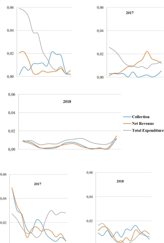
Figure 1 shows the results of the forecast error as measured by MAPE. The expected behavior of the curve would be decreasing, indicating that as it approaches the month with the value realized, the forecast error would be decreasing. This occurred, for example, with total expenditure in 2016. In January 2016, MAPE was 0.0591, falling to 0.022 in June 2016. However, in some cases, such as the forecast error of the total expenditure made two years in advance (two charts of the figure bottom), it is observed that the error initially reduces from 0.027 (January 2017) to 0.011 (April 2017) and then increases again (0.030 in September 2017).
More objectively, the survey authors compared prediction errors for annual data up to one year in advance and at two years. In other words, between the errors that are in the chart at the top left and the bottom chart. Among 72 possible cases (24 months for three variables), the forecast error for more recent dates was higher than the error with the most distant temporal horizon in 21 cases. A test of signal difference between the two MAPE shows that the larger the temporal horizon, the greater the forecast error. This result is in agreement with the assumption of the hypothesis H1, and corroborates with the result of the research of Deus and Mendonça (2017). This same analysis was performed with z. The errors with the shortest time horizon were lower than those with the highest horizon (29 out of 72), but the result is not as conclusive for the MAPE error. The reason for this is in the greater dispersion of the estimate when the temporal horizon is larger.
The Figure 1 shows the forecast for the annual values of the collection, net revenue and total expenditure made each month of the year. At the top, to the left, the forecast for the 2016 data; to the right, the 2017 data; down, 2018 data. In the second part of the figure, the errors for the following year.
4.2 FORECAST DISPERSION AND TIME HORIZON—H
2It is possible to verify whether the time horizon influences the dispersion in the forecast in several ways. However, because Prisma does not present the number of participants in the reports, a Levene test, which measures the equality of two variances, is not feasible. As the standard deviation can be affected by the size of the measure, we chose to use the coefficient of variation, which corresponds to the division of the deviation by the mean.
When comparing the forecast made for the following month with the forecast for two months, the dispersion of the forecasts has not show substantial modification, as measured by the signal test. A mean test was also done and there was no difference; thus, the assumption of the hypothesis H2 that the more distant the time horizon, the greater the dispersion of the estimates was rejected. One possible explanation for this result is the seasonality of the series, which may influence not only the forecast but also the errors made.
4.3 FORECAST ERROR AND DISPERSION OF THE ESTIMATE—
HYPOTHESIS H
3It was verified whether the forecast errors influence the behavior of the predictors in the following month. For this, the correlation between the prediction error (MAPE and z) and the forecast of the immediately following period was calculated. The results showed a correlation of 0.45, 0.36 and 0.03 using the MAPE and of 0.27, 0.19 and -0.11, using the measure z for the collection, net revenue and total expenditure, in that order. The correlations obtained with MAPE for the first two variables are significant. The data indicate that increases in forecast errors for a given month tend to increase the dispersion of forecasts for the following month in some cases. Moreover, when the MAPE lag increases for the total expenditure variable over one and two months, the correlation goes from 0.03 to 0.60 and 0.37, statistically significant. Therefore, the hypothesis H3 which is assumed to have a significant correlation between the error at month t and the t + 1 dispersion was not rejected. This result corroborates with Deus and Mendonça (2017), who evidenced persistence in the error of fiscal forecasting in Brazil. It is as if the economic agent adjusted his ruler, calibrating it after a great mistake.
4.4 OPTIMISTIC BIAS IN FORECASTS—HYPOTHESIS H
4A signal test was carried out to determine whether the average projections of the analysts presented values higher than the real ones, for the collection and the revenue, and the inverse, for the total expenditure. This would be a sign of optimism in projections. The number of months where the difference was favorable, the optimism hypothesis was higher, but not to the point of being considered statistically significant. Thus, contrary to An et al. (2018), Deus e Mendonça (2017) and Pina and Venes (2011) who found optimistic bias in their research, in the present study there was no optimism in the projections. Therefore, hypothesis H4, where it was expected that the value of the collection and expected revenue would be higher than the value realized, and the value of the total expenditure forecast would be lower than the value realized, was rejected. One possible explanation for this result is the fact that predictors use econometric models in prediction, which may minimize the effect of optimism.
4.5 ADDITIONAL DISCUSSION
During the execution of the research, it was expected that the presence of outliers could result in losing of quality of the projection. One method of highlighting these outliers would be through the Mahalanobis test. However, the lack of access to all forecast data makes it impossible. An alternative, less scientific, is to use the median instead of the mean in the error estimate. The median has, among its properties, the fact that it is not affected by these extreme values. For Armstrong and Collopy (1992) the use of the median is a way to remove all values above and below the mean value. Thus, MAPE was calculated for the three variables using the median in place of the mean in Expression 2. The results of 0.033, 0.060 and 0.049 (Table 1, first row) were replaced by 0.031, 0.055 and 0.043. Thus, an improvement in the forecast of the variables occurred. The difference between the values was not expressive, indicating that the presence of outliers can not be considered as a factor of reduction in the quality of the forecasts.
A second analysis concerns the forecasts called Podium. In this case, the Ministry of Economy discloses the guesses of the three “best” economic agents. By the concept of reversion to the mean, the estimate of these agents should not be substantially better than the ones of the other agents. However, if these agents have some special skills in making forecasts, such as those investigated by Tetlock and Gardner (2015), one would expect their results to be better than the overall average. If the belief is in the wisdom of the masses, according to Surowiecki (2004), the overall average should announce a better performance over time. As the disclosure of the Podium began in mid-2016, MAPE was calculated for the three variables analyzed (collection, net revenue and total expenditure) for these agents,
being N = 304. The mean of the agents for the three variables was (0.0338, 0.0560 e 0.04). For the Podium analysts this mean was (0.0506, 0.0876 e 0.0651). A mean test between each pair of values revealed that the predictions of the experts do not differ from the average, except for variable net revenue.
Finally, it was verified the evolution of errors over time. Should there be a learning process, it is expected that on average the error decreases over time. One way to verify this is by doing two regressions, where MAPE and z would be the dependent variables and time would be the independent variable. Should the angular coefficient be negative and significant, this would indicate that the forecasts would be improving over time, due to the reduction of the error. If the angular coefficient is positive and significant, this corresponds to a reduction in the quality of forecasts over time. If the angular coefficient is not significant it can be argued that there is no learning in the forecasts. The results are presented in Table 2. In all six models (three variables for the two measures of error) the value of the p-value of the angular coefficient was high. Despite this, the coefficients presented a negative signal, indicating a possible improvement in the projections. From this result, it was taken from the six regressions at constant, corresponding o Model 2 column of Table 2. The p-value of the coefficient showed significant, at 1%, for the six regressions. This indicates an improvement in the explanation of error behavior over time. However, as the signal is positive in all cases, the measure of error has increased over time. This result was not expected, since a learning of the economic agents from time to time was expected. A possible explanation for this fact may be the presence of external variables, which increased the uncertainties of the economic environment and the forecasts made.
Table 2
Temporal evolution of fiscal variables errors
Model 1 Model 2
Measure and Y Constant Angular Coeffi-cient p-value Angular Coeffi-cient p-value
MAPE Collection 0.048 -0.001 0.448 0.001 0.004 Net Revenue 0.085 -0.001 0.115 0.002 0.001 Total Expenditure 0.056 -0.001 0.208 0.002 0.000 z Collection 0.865 -0.006 0.677 0.030 0.000 Net Revenue 1.156 -0.009 0.580 0.038 0.000 Total Expenditure 1.063 -0.008 0.483 0.035 0.000
Note. Two models were calculated for each of the three variables and for the two types of errors, resulting in 12 regressions. Model 1 corresponds to linear regression with the presence of the constant. In model 2 the constant was withdrawn.
The results obtained in this research are partially in accordance with what was expected, as presented throughout of the analysis. However, the expected optimistic bias was not observed, contradicting the literature (An et al., 2018; Piza, 2019). Likewise, the quality of the forecasts does not seem to have been relevant, as evidenced by Brogan (2012) and Deus and Mendonça (2017). In the same way, the projection of the “best” predictors did not differ from the average, contrary to Tetlock and Gardner (2015), but corroborating Surowiecki (2004).
5 CONCLUDING REMARKS
The objective of this study was to investigate determinant factors of the forecast errors of market analysts for Brazilian fiscal variables. For this, the data of the collection, net revenue and total expenditure made available in the Prisma Fiscal were used. The Prisma Fiscal collects and discloses information on forecasts market analysts of the Brazilian public finances variables. By using this information and comparing it with the values that actually occurred, this research intended to verify whether: the further distant in time, the greater the prediction error; the further distant in time, the greater the dispersion between estimates; the increase in error has an effect on the dispersion of the forecasts of the experts; and whether there is an optimistic bias in these predictions. The forecasting process is so complex and nuanced that the results of this research can not be considered as conclusive. There is every reason to believe that there is an increase in error, the further the temporal horizon, but this does not seem to occur with forecasts deviations. Likewise, the increase in forecast error tends to increase dispersion in the following period; this is as if the agents were calibrating their predictive models. However, there is no optimistic bias in the forecasts.
In addition, three additional tests were performed. The first one found that the possible presence of outliers in the forecasts did not substantially affect the results. The second one analyzed whether the forecasts of Podium agents, those who have performed well in the past, ensure that their predictive models are better than average in future forecasts. The tests indicate that this is not true, being closer to a reversal situation to the average. The last test tried to verify whether there was an improvement in the forecasts, through the reduction of errors, over time. The result showed that the reverse occurred in the period of time studied: forecasts errors are increasing over time.
Several are the practical implications of the research. Broadly, it can be concluded that the prediction error in variables of the area of public finances and public accounting can be affected by several factors. Even relations apparently obvious, such as H2, were not found in the analysis performed in this research. The present research used value of z as a criterion for measuring the forecast error. This value has not been used in this type of investigation
and the results have shown promise. Some previous conclusions, expected from the study of the literature, did not occur, and the research makes contributions towards speculating the reasons for the results obtained. In this sense, this research can make a contribution to the area of public finance and public accounting by studying some relevant variables existing in the area’s forecasts.
REFERENCES
An, Z., Jalles, J. T., Loungani, P., & Sousa, R. M. (2018). Do IMF fiscal forecasts add value?
Journal of Forecasting, 37, 650-665.
Armstrong, J. S., & Collopy, F. (1992). Error Measures for Generalizing About Forecasting Methods: Empirical Comparisons. International Journal of Forecasting, 8(1), 69-80. Asimakopoulos, S., Paredes, J., & Warmedinger, T. (2020). Real-Time Fiscal Forecasting
Us-ing Mixed-Frequency Data. Scandinavian Journal of Economics, 122(1), 369-390.
Banco Central do Brasil. (2018). Estoque de swap cambial caiu nos últimos dois anos. Recu-perado de https://www.bcb.gov.br/noticiasporano
Banco Central do Brasil. (2019). Focus Relatório de Mercado. Recuperado de https://www. bcb.gov.br/publicacoes/focus
Brasil. Ministério da Economia. (2018). Prisma Fiscal—Nota Metodológica. Recuperado de http://www.fazenda.gov.br/prisma-fiscal/prisma-fiscal
Brasil. Ministério da Fazenda. (2016). Resultado do Tesouro Nacional. Secretaria do Tesouro
Nacional, 2(10). Recuperado de http://www.planalto.gov.br/ccivil_03/decreto-lei/del0200.
htm
Brogan, M. (2012). The politics of budgeting: evaluating the effects of the political election cycle on state-level budget forecast errors. Journal Public Administration, 36(1), 84-115. Clement, M. (1999). Analyst forecast accuracy. Journal of Accounting and Economics, 27(3),
285-303.
Conselho Federal de Contabilidade. (2016). NBC TSP—Estrutura Conceitual para
Elab-oração e Divulgação de Informação Contábil de Propósito Geral pelas Entidades do Setor Público. Recuperado de
Costa, A. E., Filho, & Rocha, F. (2010). Como o mercado de juros futuros reage à comuni-cação do Banco Central? Economia aplicada, 14(3), 265-292.
Costa, E. A. A. (2011). Fatores institucionais que influenciam a previsão das receitas
orça-mentárias: Um estudo de caso dos governos estuais brasileiros (Dissertação de
mestra-do). Universidade de Brasília, Brasília, DF.
Deus, J. D. B. V., & Mendonça, H. F. (2017). Fiscal forecasting performance in an emerging economy: An empirical assessment of Brazil. Economic Systems, 41(3), 408-419.
Diebold, F., & Mariano, R. (2012). Comparing predictive accuracy. Journal of Business &
Economics Statistics, 20(1), 134-144.
Flyvbjerg, B. (2011). Over Budget, Over Time, Over and Over Again: Managing Major Proj-ects. In P. W. G. Morris, J. Pinto, & J. Söderlund (Eds.), The Oxford Handbook of Project
Management (pp. 321-344). Oxford: Oxford University Press.
Fortis, M. F. A., & Gasparini, C. E. (2017). Plurianualidade orçamentária no Brasil:
Diagnósti-co, rumos e desafios. Brasília, DF: Enap.
Giacomini, R., Skreta, V., & Turen, J. (2020). Heterogeneity, inattention, and bayesian updates. American Economic Journal: Macroeconomics, 12(1), 282-309.
Guillén, O. T. C., Hecq, A., Issler, J. V., & Saraiva, D. (2015). Forecasting multivariate time series under present-value model short- and long-run co-movement restrictions.
Interna-tional Journal of Forecasting, 31, 862-875.
Hope, O. (2003). Disclosure Practices, enforcement of accounting standards, and analysts´ forecast accuracy. Journal of Accounting Research, 41(2), 235-272.
Hyndman, R. J., & Koehler, A. B. (2006). Another look at measures of forecast accuracy.
In-ternational Journal of Forecasting, 22, 679-688.
Jonung, L., & Larch, M. (2006). Improving fiscal policy in the EU: The case for independent Forecasts. Economic Policy, 21(47), 492-534.
Kim, S., & Kim, H. (2016). A new metric of absolute percentage error for intermittent demand forecasts. International Journal of Forecasting, 32, 669-679.
Martinez, A. L. (2007). Determinantes da acurácia das previsões dos analistas do mercado de capitais. UnB Contábil, 10(2).
Mckenzie, J. (2011). Mean absolute percentage error and bias in economic forecasting.
Eco-nomics Letters, 113, 259-262.
Merola, R., & Pérez, J. J. (2013). Fiscal forecast errors: Governments vs independent agen-cies? European Journal of Political Economy, 32, 285-299.
Pina, A., & Venes, N. (2011). The political economy of EDP fiscal forecasts: An empirical as-sessment. European Journal of Political Economy, 27, 534-546.
Pires, M. C. C. (2006). Credibilidade na política fiscal: Uma análise preliminar para o Brasil.
Revista Economia Aplicada, 10(3), 367-375.
Piza, E. C. (2019). Determinantes dos desvios de execução da política fiscal no Brasil.
Revis-ta de Economia e Agronegócio, 17(2).
Reitano, V., Jones, P., Barrett, N., & Fowles, F. (2019). Forecast bias and capital reserves accumulation. The Palgrave Handbook of Government Budget Forecasting, 377-396. Surowiecki, J. (2004). The wisdom of crowds: Why the many are smarter than the few and
how collective wisdom shapes business, economies, societies, and nations. New York:
An-chor Books.
Tetlock, P. E., & Gardner, D. (2015). Superforecasting: The Art and Science of Prediction. New York, NY: Crown Publishing.
Como citar este artigo: ABNT
SOUZA, Francisca Aparecida de; SILVA, César Augusto Tibúrcio; ALVES, Karla Roberta Castro Pinheiro. Factors determining the forecast errors of market analysts for fiscal variables in Brazil. RACE, Revista de Administração, Contabilidade e Economia, Joaçaba: Editora Unoesc, v. 19, n. 2, p. 227-248, maio/ago. 2020. Disponível em: http:// editora.unoesc.edu.br/index.php/race. Acesso em: dia/mês/ano.
APA
Souza, F. A. de, Silva, C. A. T., & Alves, K. R. C. P. (2020). Factors determining the forecast errors of market analysts for fiscal variables in Brazil. RACE, Revista de Administração,
Contabilidade e Economia, 19(2), 227-248 Recuperado de http://editora.unoesc.edu.br/