The importance of friction in mountain wave drag amplification by scorer parameter resonance

wave drag amplification by Scorer 

parameter resonance 

Article 

Accepted Version 

Teixeira, M. A. C., Argaín, J. L. and Miranda, P. M. A. (2012) 

The importance of friction in mountain wave drag amplification 

by Scorer parameter resonance. Quarterly Journal of the 

Royal Meteorological Society, 138 (666). pp. 1325­1337. ISSN 

1477­870X doi: https://doi.org/10.1002/qj.1874 Available at 

http://centaur.reading.ac.uk/29232/ 

It is advisable to refer to the publisher’s version if you intend to cite from the 

work.  See 

Guidance on citing  

.

To link to this article DOI: http://dx.doi.org/10.1002/qj.1874 

Publisher: Royal Meteorological Society 

All outputs in CentAUR are protected by Intellectual Property Rights law, 

including copyright law. Copyright and IPR is retained by the creators or other 

copyright holders. Terms and conditions for use of this material are defined in 

the 

End User Agreement  

. 

www.reading.ac.uk/centaur  

Central Archive at the University of Reading 

Reading’s research outputs online

The importance of friction in mountain wave drag

amplification by Scorer parameter resonance

M. A. C. Teixeira

_{, J. L. Arga´ın}

_{, P. M. A. Miranda}

∗_{Correspondence to: Miguel A. C. Teixeira, Centro de Geof´ısica da Universidade de Lisboa,}

Edif´ıcio C8, Campo Grande, 1749-016 Lisbon, Portugal. E-mail: [email protected]

A mechanism for amplification of mountain waves, and their associated drag,

by parametric resonance is investigated using linear theory and numerical

simulations. This mechanism, which is active when the Scorer parameter

oscillates with height, was recently classified by previous authors as intrinsically

nonlinear. Here it is shown that, if friction is included in the simplest possible

form as a Rayleigh damping, and the solution to the Taylor-Goldstein equation

is expanded in a power series of the amplitude of the Scorer parameter

oscillation, linear theory can replicate the resonant amplification produced by

numerical simulations with some accuracy. The drag is significantly altered

by resonance in the vicinity of

n/l

= 2, where l

is the unperturbed value of

the Scorer parameter and

n is the wavenumber of its oscillation. Depending

on the phase of this oscillation, the drag may be substantially amplified or

attenuated relative to its non-resonant value, displaying either single maxima

or minima, or double extrema near

n/l

= 2. Both nonhydrostatic effects and

friction tend to reduce the magnitude of the drag extrema. However, in exactly

inviscid conditions, the single drag maximum and minimum are suppressed.

As in the atmosphere friction is often small but non-zero outside the boundary

layer, modelling of the drag amplification mechanism addressed here should be

quite sensitive to the type of turbulence closure employed in numerical models,

or to computational dissipation in nominally inviscid simulations. Copyright c

°

0000 Royal Meteorological Society

Key Words: Internal gravity waves, Parametric resonance, Dissipative processes, Linear theory, Asymptotic expansion

Received

Copyright c° 0000 Royal Meteorological Society Q. J. R. Meteorol. Soc. 00: 2–18 (0000) Prepared using qjrms4.cls

1. Introduction

Gravity wave drag is one of the key phenomena that must be parametrized in global weather prediction and climate models. A multitude of processes affect this topographically generated force, making it exceed leading-order estimates from linear theory, in what are called ‘high-drag states’. It is important to understand ‘high-drag enhancement mechanisms, since they provide a dominant contribution to the globally-integrated drag, having a significant impact on the deceleration of the atmospheric circulation.

In a recent paper, Wells and Vosper (2010) (hereafter referred to as WV10) assessed the accuracy of linear theory for diagnosing mountain wave drag in stratified flow over 2D ridges. The focus of their study was on situations where the actual drag might significantly exceed the drag predicted by linear theory, even for extremely low mountain heights. One such situation, identified by them, is when the spectrum of the Scorer parameter profile contains harmonics that can lead to a resonant amplification of the mountain waves. In order to isolate this effect, they considered an idealized case where a small sinusoidal perturbation is added to a constant Scorer parameter profile, with a wavelength half that of the dominant vertical wavelength of the internal gravity waves. In that case, they showed that the drag may exceed its linear value by a factor of 2 or more, depending on the phase of the Scorer parameter oscillation. Since the linear model of WV10 failed to predict this behaviour, they attributed the drag amplification to nonlinear wave-wave interactions, as investigated originally by Phillips (1968) in an oceanographic context, and more recently by Nance and Durran (1998) and Lee et al. (2006). However, although in WV10’s study the nonlinear drag was normalized by the corresponding linear value, the behaviour of the linear drag was never explicitly shown for this case.

The characteristics of the drag amplification outlined above immediately suggest that it results from parametric resonance, since the role played by the Scorer parameter in the Taylor-Goldstein equation is akin to that of

the coefficient multiplying the position in an equation describing a simple harmonic oscillator. This resonance is therefore of a different kind from those investigated, for example, by Miranda and Valente (1997), Wang and Lin (1999), Leutbecher (2001), and Teixeira et al. (2005, 2008), which resulted from discontinuities in the mean atmospheric parameters, or their derivatives. It is also different from the resonance investigated by Grubiˇsi´c and Stiperski (2009) and Stiperski and Grubiˇsi´c (2011), which results from the horizontal distribution of the topographic forcing of lee waves (see also Grisogono et al., 1993; Vosper, 1996).

One aim of the present paper is to address an idealized situation akin to that considered by WV10 using linear theory, thus showing that the kind of resonance they investigated is possible under its assumptions, and can lead to very substantial drag enhancement. A second aim is to show how the inclusion of friction in the model is crucial to obtain a drag behaviour qualitatively similar to that produced in the numerical simulations of WV10, or roughly similar ones. Friction fulfils two roles: firstly, it limits the drag magnitude in resonant conditions (something that is presumably effected by nonlinear processes in more realistic circumstances). Secondly, since friction prevents the singular behaviour of the drag that occurs in inviscid conditions, it also widens the drag extrema at resonance, rendering them detectable in a representation similar to that of Figure 9 of WV10.

We therefore speculate that inviscid linear theory, such as employed by WV10 in part of their calculations, should be unable to properly represent this type of resonance. For the same reasons, it is likely that the magnitude of the drag enhancement in resonant conditions is quite sensitive to dissipative processes in numerical models, be they due to the type of adopted turbulence closure, or to the more or less diffusive character of the discretization scheme employed. These conjectures are tested in the present study by comparing results from linear theory, where a small sinusoidal variation of the Scorer parameter is treated using

a perturbation approach, and fully nonlinear numerical simulations of the same situation.

This paper is organized as follows: section 2 contains a description of the analytical theoretical model and of the numerical simulations. In section 3, the variation of the drag with friction and nonhydrostatic effects is explored, and the pressure and velocity fields are analyzed. Results from the theoretical model and from the numerical simulations are compared. Finally, section 4 summarizes the main findings of this study.

2. Methodology

2.1. Analytical drag model

Stationary, non-rotating flow over a 2D mountain ridge is considered. The Boussinesq approximation is assumed, and the equations of motion are linearized with respect to a reference state, but the flow is assumed to be nonhydrostatic. Friction, which turns out to be a crucial effect, is included in the simplest possible form as a Rayleigh damping. The adopted equations of motion (cf. Lin, 2007, sections 5.1 and 13.2.2) are :

U∂u ∂x + w dU dz = − 1 ρ0 ∂p ∂x− λu, (1) U∂w ∂x = − 1 ρ0 ∂p ∂z+ b − λw, (2) U∂b ∂x+ N 2_{w = 0, (3)} ∂u ∂x+ ∂w ∂z = 0. (4)

Here x is the horizontal coordinate perpendicular to the ridge, z is the height, U (z) is the incoming wind velocity (aligned with x), N (z) is the Brunt-V¨ais¨al¨a frequency of the incoming flow, ρ0 is a reference density (assumed to be constant) and λ is a (constant) Rayleigh damping coefficient. u, w, p and b are, respectively, the horizontal velocity, vertical velocity, pressure and buoyancy perturbations associated with the mountain waves. Note that, for simplicity, friction terms are only included in the momentum equations and not in the heat balance

equation. It can be shown that, for the small values of λ to be considered, this has a negligible effect on the model behaviour apart from a rescaling of λ by a factor of 2 (if the Rayleigh coefficient for heat was assumed to be the same).

Equations (1)-(4) may be differentiated and combined, yielding a single equation for w. All perturbed variables may be expressed as 1D Fourier integrals. For example, w can be written (see, e.g. Lin, 2007, Appedix 5.1)

w(x, z) =

Z _+∞

−∞

ˆ

w(k, z)eikx_{dk, (5)}

where ˆw is the corresponding Fourier transform, k is the

horizontal wavenumber and i =√−1. From (1)-(4) and (5),

it can be shown that ˆw satisfies

ˆ w00₊ Ã l2 1 − i λ U k − k2 ! ˆ w = 0, (6)

where l2_{= N}2_/U2_{− U}00_{/U is the square of the Scorer}

parameter, and the primes denote differentiation with respect to z.

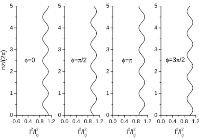
In order to reproduce conditions akin to those considered in Figure 9 of WV10, the Scorer parameter squared is assumed here to take the form:

l2_{= l}2

0{1 + ε cos(nz + φ)}, (7)

where l2

0is a constant, ε is a small dimensionless parameter, n is the vertical wavenumber of the perturbation imposed on l2

0 and φ is the corresponding phase. Equation (7) defines a Scorer parameter that oscillates with height with a relatively small amplitude (see Figure 1).

For the particular case λ = 0, (6) along with (7) is a Mathieu equation, which describes parametric resonance, and its solutions must be expressed in terms of Mathieu functions (Abramowitz and Stegun, 1972). However, when

ε is assumed to be small (it takes the value 0.1 in WV10), it

is possible to solve (6) approximately in terms of elementary functions using a perturbation approach, by expanding its

0.0 0.4 0.8 1.2 0 1 2 3 4 5 0.0 0.4 0.8 1.2 0 1 2 3 4 5 0.0 0.4 0.8 1.2 0 1 2 3 4 5 φ=3π/2 φ=π φ=π/2 n z /( 2 π ) l2/l2₀ φ=0 0.0 0.4 0.8 1.2 0 1 2 3 4 5 l2/l2₀ l2/l2₀ l2/l2₀

Figure 1. Variation of the normalized square of the Scorer parameter as a function of normalized height according to (7), for ε = 0.1 and four values of φ.

solution in a power series of ε:

ˆ

w = ˆw0+ ε ˆw1+ ε2wˆ2+ ... . (8)

In fact, for the present purposes, and as will be seen next, it is sufficient to consider this series only up to first-order in ε. If (7) and (8) are introduced into (6), the following two equations result at zeroth- and first-order in ε:

ˆ w00 0 + Ã l2 0 1 − i λ U k − k2 ! ˆ w0= 0, (9) ˆ w00 1 + Ã l2 0 1 − i λ U k − k2 ! ˆ w1 = − ˆw0 l 2 0 1 − i λ U k cos(nz + φ). (10)

In this formulation, it becomes especially clear that the zeroth-order solution ˆw0, in conjunction with the perturbation to the Scorer parameter, acts as a source term for the first-order solution ˆw1. Thus this equation set already contains the possibility of resonance.

The solution to (9) is (see Lin, 2007, section 5.2.1)

ˆ

w0= iU0kˆheimz, (11)

where U0= U (z = 0), ˆh is the Fourier transform of the surface elevation and m is the vertical wavenumber of the

internal gravity waves, defined, using (9) and (11), as:

m2= l 2 0 1 − i λ U k − k2. (12)

In the above passage it was implicitly assumed that U is constant, otherwise (11) and (12) would not be valid in the generic case λ 6= 0. However, if λ = 0, this assumption is not necessary, so U will continue to be treated as a function of z in the following, for maximum generality. The coefficient multiplying the exponential in (11) takes into account the boundary condition at the surface ˆw0(z = 0) = iU0kˆh and the sign of m is determined by the upper radiation boundary condition. If m is decomposed into its real and imaginary parts mRand mI

m = mR+ imI (13)

(which are nonzero simultaneously as long as λ 6= 0), then it can be shown that the definitions of mRand mI that are

physically consistent (see Appendix A) are:

mR= 1 √ 2 λ U kl20 1 + λ2 U2_k2 ( k2− l 2 0 1 + λ2 U2_k2 + v u u t à l2 0 1 + λ2 U2_k2 − k2 !2 + λ2 U2_k2 l4 0 ¡ 1 + λ2 U2_k2 ¢2    −1 2 , (14) mI = √1 2 ( k2− l 2 0 1 + λ2 U2_k2 + v u u t à l2 0 1 + λ2 U2_k2 − k2 !2 + λ2 U2_k2 l4 0 ¡ 1 + λ2 U2_k2 ¢2    1 2 , (15)

which result from (12) and (13). In (15) mI > 0, as it must

be for the wave perturbation to decay with height according to (11) and (13). On the other hand, in (14) mR has the

same sign as U k, which corresponds to upward wave energy propagation (see e.g. Teixeira and Miranda, 2005, 2006).

Inserting (11) into (10), the solution to the latter equation (see Appendix B) is

ˆ w1= U0kˆh 2m l2 0 1 − i λ U k ·Z _+∞ 0

cos(ns + φ)e2imsds סeimz_{− e}−imz¢ + Z z 0 cos(ns + φ) n e−im(z−2s)_{− e}imzo_ds ¸ , (16)

where it has been again assumed that U is constant when λ 6= 0. This form emphasizes upward and downward propagating components of the first-order wave perturbation (corresponding to exponential terms with positive and negative exponents that are a function of z, respectively). The solution (16) satisfies the lower boundary condition

ˆ

w1(z = 0) = 0 and the upper boundary condition that the wave energy decays or propagates upward as z → +∞. It can be seen from (16) that the upward and downward propagating wave components are of similar magnitude at z = 0, whereas the downward propagating component vanishes as z → +∞. The integrals in (16) may be calculated analytically, yielding

ˆ w1= − U0kˆh 4m2_{− n}2 l2 0 1 − i λ U k · 2m n {sin(nz + φ) − sin φ} + i {cos(nz + φ) − cos φ}] eimz. (17)

In this equation it can already be seen that parametric resonance will happen for n = ±2mR, since 4m2− n2

appears in a denominator on the right-hand side. When

λ = 0, m2 _{is real and there is the possibility that this} denominator becomes zero. When λ 6= 0, however, (15) shows that mI is never zero, even if the waves are vertically

propagating. So ˆw1 will not diverge to infinity in those circumstances (which would invalidate the power series solution), but will be strongly amplified for relatively small

λ.

The focus in the present study is on the calculation of the surface drag associated with the mountain waves. The drag per unit spanwise width of the ridge is given by

(Teixeira and Miranda, 2004)

D = Z _+∞ −∞ p(z = 0)∂h ∂xdx = 2πi Z _+∞ −∞ k ˆp∗(z = 0)ˆhdk, (18) where h is the surface elevation, the asterisk denotes complex conjugate, and Parseval’s theorem has been used. In order to calculate the drag, it is therefore necessary to obtain the pressure perturbation at the surface. Using (1) and (4), the Fourier transform of the pressure perturbation ˆ

p, which is related to p in the same way as ˆw is related to w

in (5), is given by ˆ p = iρ0 k ½ U0_{w − Uˆ} µ 1 − i λ U k ¶ ˆ w0 ¾ . (19)

An inviscid (λ = 0) but 3D version of (19) was presented, for example, by Teixeira and Miranda (2006) as their Eq. (8). From (8) and (19), it is clear that ˆp may also be

expressed as a power series of ε, as

ˆ

p = ˆp0+ εˆp1+ ε2pˆ2+ ... . (20)

If (11) is differentiated and evaluated at z = 0, and used in (19), it can be shown (see Appendix C) that

ˆ p0(z = 0) = ρ0U02ˆh ½ i µ mR+ λ U kmI ¶ −mI+ λ U kmR− U0 0 U0 ¾ , (21) where U0

0= U0(z = 0), and (13) and (20) were also used. Equation (17) may also be differentiated, evaluated at z = 0, and inserted into (19) (see Appendix C), yielding

ˆ p1(z = 0) = − ρ0U 2 0l02ˆh (4m2 R− 4m2I − n2)2+ 64m2Rm2I ×£i©8nmRmIsin φ − 2 ¡ 4m2 R+ 4m2I− n2 ¢ ×mRcos φ} − ¡ 4m2 R− 4m2I− n2 ¢ n sin φ −2¡4m2 R+ 4m2I− n2 ¢ mIcos φ ¤ , (22)

where, again, (13) and (20) have been used.

In the case of an orography that is symmetric in x, ˆh is real and so, according to (18), only the imaginary parts of ˆ

p0and ˆp1contribute to the drag. The drag is obviously also expressed as a power series in ε,

D = D0+ εD1+ ε2D2+ ... . (23)

Here the total drag, which is only calculated up to first-order, is normalized by the drag in the absence of resonance,

D0. This is accomplished by inserting (21) and (22) into (20) and using the latter equation in (18). The final result is

D D0 = 1 + ε D1 D0 = 1 +R_+∞ 2ε 0 k0|ˆh0|2 ¡ m0 R+U kλa0m0_I ¢ dk0 Z +∞ 0 k0_|ˆh0_|2 ×m0 R (4m02 R+ 4m 0₂ I − n 0₂ ) cos φ − 4n0_m0 Isin φ (4m0₂ R− 4m 0₂ I − n 0₂ ) + 64m0₂ Rm 0₂ I dk0_, (24) where k0_{= ka, ˆh}0 _{= ˆh/(h} 0a), m0R= mR/l0, m0I = mI/l0 and n0_{= n/l}

0are dimensionless parameters and functions defined in terms of the corresponding dimensional quantities, specified previously. a and h0are, respectively, a representative width and height of the orography.

Although the results of the model would not be essentially changed by adopting a different form for the surface elevation, following WV10 it will be assumed here that the orography is a bell-shaped ridge:

h = h0 1 + (x/a)2, ⇒ ˆh 0₌ 1 2e −|k0_| . (25)

The normalized drag given by (24) is a function of five dimensionless parameters n/l0, φ, ε, l0a and λa/U . Since, as was seen above, resonance occurs when n = ±2mR,

and |mR| ≈ l0when the flow is approximately inviscid and hydrostatic (i.e. when l0a is large and λa/U is small – see (14)), resonance will occur in the vicinity of n/l0= 2. For that reason, the drag will be represented next as a function of n/l0, for particular values of the other flow parameters.

2.2. Numerical simulations

Numerical simulations were performed using the FLEX numerical model, which is a 2D nonlinear and nonhy-drostatic microscale to mesoscale model using generalized curvilinear coordinates (see Arga´ın et al., 2009). For all simulations, and as in WV10, the rotation of the Earth was neglected and flow over a bell-shaped mountain (25) with

a = 10km, h0= 10m was considered. The unperturbed Brunt-V¨ais¨al¨a frequency and the mean wind speed were

N0= 0.01s−1 and U = 20m s−1. Therefore, the flow was strongly linear (N0h0/U = 5 × 10−3) (at least in non-resonant conditions) and reasonably hydrostatic (N0a/U = 5). When testing nonhydrostatic effects, a = 20km and a = 4km, were also employed, so that N0a/U = 10 (strongly hydrostatic flow) or N0a/U = 2 (strongly nonhydrostatic flow). The adopted Scorer parameter profile was con-structed according to (7), with l0= N0/U and its vertical oscillation was imposed by adding a perturbation to N2

0, of relative amplitude ε = 0.1. This approach differs from that of WV10, where the perturbation is imposed on U instead.

The model was run in a domain of length 24a in the horizontal (≈ 240km for a = 10km) by 3.5λz in the

vertical (λz= 2πU/N0 is the vertical wavelength of the gravity waves). This corresponds to ≈ 44km for the values of N0 and U quoted above. A grid of 160 × 525 points, with a resolution of 0.15a in the horizontal (1.5km for a = 10km) and λz/150 in the vertical (≈ 84m for the values of

N0 and U quoted above) was used. Lateral sponges with width 4a and a sponge at the top of the domain with depth 1.5λzwere also employed.

The model was run with a time step of 2s for a period of up to 500a/U (corresponding to 69 hours for a = 10km and U = 20m s−1_{), until the drag stabilized to a constant}

value. In many cases, the time necessary for this to happen was not larger than 120a/U , or 17 hours, but in resonant conditions it became considerably larger (cf. WV10).

Most of the simulations were carried out in inviscid mode, that is, using a free-slip boundary condition at

the surface and no turbulence closure. The simulations of section 3.5 used a no-slip boundary condition, and either a Smagorinsky-type turbulence closure (Lilly, 1962) or a K-ε turbulence closure. In these cases, Monin-Obukhov profiles were used to initialize the model up to the top of the boundary layer height (which is consistent with the absence of rotation). A roughness length of z0= 0.05m, a Monin-Obukhov length of LM O= 255m and a friction velocity

of u∗= 0.46m s−1 were employed. The latter two values

were determined using the method proposed by Arga´ın et

al. (2009). In these simulations, the drag took considerably

less time to stabilize than in inviscid conditions (at most 150a/U or 21 hours in all cases).

3. Results

3.1. The importance of friction

Since friction appears to be of crucial importance in the type of flow being considered, its effect on the behaviour of the analytical model presented above will be analyzed first, and compared with nominally inviscid numerical results.

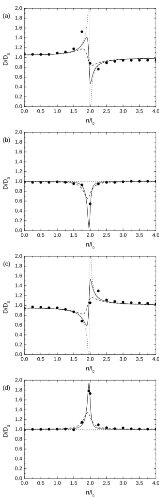
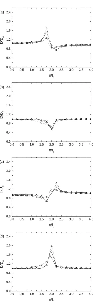
Figure 2 shows the normalized drag, as given by (24), for ε = 0.1 and l0a = 5 (as in WV10), for three values of the friction coefficient λa/U (lines). Also shown are results for the same conditions, but from inviscid simulations of the FLEX numerical model (symbols). Although, in all cases displayed, the normalized drag only departs substantially from 1 in the vicinity of n/l0= 2, which is consistent with the existence of parametric resonance, the behaviour is strongly dependent on φ. For φ = 0 (Figure 2(a)), there is a drag maximum to the left of n/l0= 2, followed by a minimum to the right of n/l0= 2. The magnitude of these extrema increases as λa/U decreases. In Figure 2(b), where φ = π/2, there is a single drag minimum, of larger magnitude than the extrema displayed in Figure 2(a), approximately centred on n/l0= 2 (slightly to the left). The magnitude of this minimum increases as λa/U decreases, but the minimum vanishes altogether for λ = 0. For φ = π (Figure 2(c)) and φ = 3π/2 (Figure 2(d)) the behaviour

0.0 0.5 1.0 1.5 2.0 2.5 3.0 3.5 4.0 0.0 0.2 0.4 0.6 0.8 1.0 1.2 1.4 1.6 1.8 2.0 D /D 0 n/l₀ (a) 0.0 0.5 1.0 1.5 2.0 2.5 3.0 3.5 4.0 0.0 0.2 0.4 0.6 0.8 1.0 1.2 1.4 1.6 1.8 2.0 (b) D /D 0 n/l₀ 0.0 0.5 1.0 1.5 2.0 2.5 3.0 3.5 4.0 0.0 0.2 0.4 0.6 0.8 1.0 1.2 1.4 1.6 1.8 2.0 (c) D /D 0 n/l₀ 0.0 0.5 1.0 1.5 2.0 2.5 3.0 3.5 4.0 0.0 0.2 0.4 0.6 0.8 1.0 1.2 1.4 1.6 1.8 2.0 (d) D /D 0 n/l₀

Figure 2. Normalized drag as function of n/l0for ε = 0.1, l0a = 5 and various values of λa/U , from (24) and from the FLEX numerical model. Dotted line: (24) with λa/U = 0, solid line: (24) with λa/U = 2 × 10−2_{, dashed line: (24) with λa/U = 0.1, symbols: FLEX. (a) φ = 0,}

(b) φ = π/2, (c) φ = π, (d) φ = 3π/2.

of the drag predicted by (24) is exactly symmetric with respect to the line D/D0= 1 relative to that displayed in Figure 2(a) and 2(b), respectively. Hence, for φ = π there is a drag minimum followed by a maximum, whereas for

φ = 3π/2 there is a single maximum. This last maximum,

which is perhaps the most relevant result from the viewpoint of drag parametrization, has the same peculiar behaviour as the minimum. Namely, while it becomes higher as

λa/U decreases, it vanishes for λ = 0. It should be noted

that the drag minima predicted by (24) at φ = 0, φ =

π/2 or φ = π would become negative for sufficiently low λa/U , an obviously unphysical result which stems from the

limitations of the perturbation approach employed in the analytical model.

The results from the FLEX numerical model are broadly in agreement with the analytical model for λa/U = 2 × 10−2_{. They cover a much more limited number of}

values of n/l0, and for that reason are not able to sample as effectively the drag variation near the peaks. For example, since the drag minimum in Figure 2(b) and the drag maximum in Figure 2(d) occur slightly below n/l0= 2, they are not perfectly captured in the numerical simulations. Unlike in the analytical model, the magnitude of the drag minimum in Figure 2(b) is smaller than the magnitude of the drag maximum in Figure 2(d), essentially because the drag cannot become negative in the numerical simulations. Nevertheless, apart from an underestimation of the drag by (24) for φ = 0 at n/l0= 1.75, the agreement between both models is quite good, even quantitatively. This means that a simple Rayleigh damping is able to capture the essential aspects of frictional effects in the present flow. It also means that, while being nominally inviscid, the simulations of the FLEX model obviously contain a small amount of numerical diffusion. Preliminary tests, where the FLEX model was run at a higher resolution, suggest that the drag extrema existing near n/l0= 2 become more pronounced, which is consistent with a decrease of computational dissipation, but further tests are required to confirm the robustness of this behaviour.

The drag maximum in the inviscid numerical results of WV10, presented in their Figure 9, is slightly larger than that in Figure 2(d), but these results are not directly comparable with ours, since WV10 imposed a perturbation on U rather than on N to produce the vertical oscillations of the Scorer parameter (see section 4).

The present results suggest that friction, which always exists in reality, is essential for the existence of the drag maximum for φ = 3π/2 and of the drag minimum for φ =

π/2. Curiously, that is not the case for the double extrema

produced for φ = 0 or φ = π, which were overlooked by WV10, but are essentially inviscid in the present framework (see Figure 2(a) and 2(c)). The possibility that a modulation of the drag with n/l0 may be produced when λ = 0 for φ = π/2 or φ = 3π/2 if the wave solution is considered up

to higher order in ε cannot be ruled out, but when ε = 0.1 this should amount to a relatively small correction, since the following power series coefficient is ε2_{= 0.01.}

The mathematical reason for the behaviour of the drag in the analytical model can be sought in (24). When

φ = π/2 or φ = 3π/2, cos φ = 0 and so only the second

term in the numerator of the fraction inside the integral is non-zero. This term contains m0

I and is multiplied by m0R

outside the fraction, so it only gives a non-zero contribution to the integral when m0

R and m0I are simultaneously

non-zero. Now, in inviscid conditions, either m0

R or m0I must

be zero, i.e., the vertical wavenumber of the mountain waves must either be pure real or pure imaginary. In those circumstances, the correction to the drag due to resonance vanishes.

A clearer explanation for this behaviour can be achieved if one notes that for the case φ = 3π/2 (corresponding to a single drag maximum) the integral in

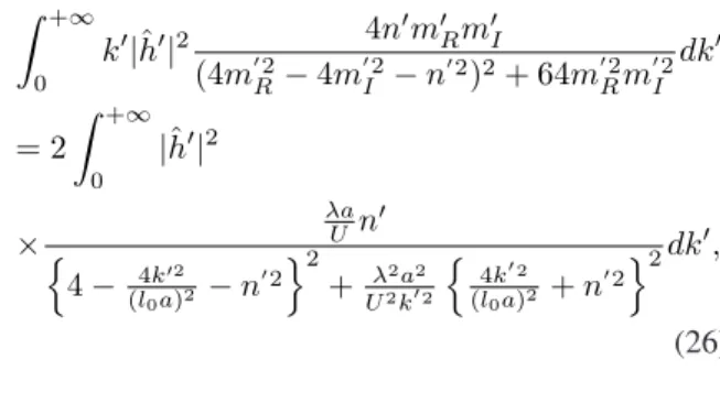
the numerator of (24) can be written Z _+∞ 0 k0|ˆh0|2 4n 0_m0 Rm0I (4m0₂ R− 4m 0₂ I − n 0₂ )2_{+ 64m}0₂ Rm 0₂ I dk0 = 2 Z _+∞ 0 |ˆh0|2 × λa Un0 n 4 − 4k02 (l0a)2 − n 0₂o2 + λ2_a2 U2_k02 n 4k02 (l0a)2 + n 0₂o2 dk0, (26)

where (14) and (15) have been used. Obviously when

λa/U → 0 this integral is zero if n/l06= 2, but it can be shown that it diverges if n/l0= 2. This becomes even more evident if the hydrostatic limit is considered. In that case, where l0a → ∞, (26) reduces to Z +∞ 0 k0_|ˆh0_|2 4n0m0Rm0I (4m0₂ R− 4m 0₂ I − n 0₂ )2_{+ 64m}0₂ Rm 0₂ I dk0 = 2 Z +∞ 0 |ˆh0_|2 λaUn0 (4 − n0₂ )2₊ λ2_a2 U2_k02n 0₄dk 0_{, (27)}

and it follows immediately that the integral (27), apart from approaching zero (making D/D0= 1) when λa/U → 0 and n/l06= 2, tends to infinity proportionally to (λa/U )−1 if n/l0= 2. In fact, it can be shown from (24) and (27) that, in the latter limit

D D0 = 1 +ε 2 µ λa U ¶−1 . (28)

So, the correction to the drag due to parametric resonance behaves in this case like a Dirac delta function as

λa/U → 0, although the perturbation approach used to

obtain this result becomes invalid in that limit. Obviously, when frictional effects are excluded from the outset, this behaviour is not uncovered, since the limit λa/U → 0 is taken before the limit n/l0→ 2.

The linear model used by WV10 was based on an equation analogous to (6), but with λ = 0 (their equation (3)). The above arguments could explain the inability of these authors to obtain a drag maximum such as shown in Figure 2(d) (or a minimum such as that in Figure 2(b))

in their linear results. However, caution is necessary, since their model, although linear, was solved numerically, and the discretization scheme should introduce some spurious numerical diffusion. Additionally, as noted above, WV10 perturbed the Scorer parameter in a different way from that adopted here, which makes comparisons difficult.

Even an inviscid linear model should be able, however, to produce the double drag extrema displayed in Figure 2(a) and 2(c), since when φ = 0 or φ = π, sin φ = 0 and so only the first term in (24) in the numerator of the fraction inside the integral is non-zero, but this term does not vanish if

m0 I = 0.

The disappearance of the single drag extrema for

φ = π/2 or φ = 3π/2 is an example of a situation where λ → 0 (vanishing friction) does not coincide with λ = 0

(zero friction). Other situations of this kind exist in fluid dynamics, in connection with boundary layer theory, for example D’Alembert’s paradox. Since the real atmosphere always possesses some friction, the subtle difference between these two limits is not very relevant from an experimental perspective. But in the context of numerical modelling, it illuminates the fact that the behaviour of the drag in these resonant flows must be quite sensitive to computational diffusion in inviscid simulations, and certainly requires an adequate turbulence closure to be accurately represented (see section 3.5 below).

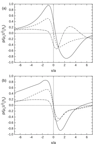
3.2. The pressure perturbation

In order to better understand the behaviour of the drag, it is worth analyzing the pressure perturbation at the surface, which is ultimately responsible for it. The cases of greatest interest are those where a single drag maximum or a single drag minimum exist, because they presumably correspond to extreme flow configurations.

Figure 3 shows the normalized pressure perturbation at the surface as a function of streamwise distance across the ridge from the analytical model (Figure 3(a)) and from the FLEX numerical model (Figure 3(b)). Cases corresponding to a drag maximum (n/l0= 2 and φ =

3π/2) and to a drag minimum (n/l0= 2 and φ = π/2) are shown, with other flow parameters similar to those used by WV10 (l0a = 5 and ε = 0.1). In the analytical model, λa/U = 2 × 10−2 _{is assumed. A case without}

resonance (ε = 0) is also presented for reference. This last case is characterized (both in Figure 3(a) and 3(b)) by a pressure distribution that is anti-symmetric with respect to the ridge axis, with a positive maximum upstream and a negative minimum downstream of the ridge, as is typical of approximately hydrostatic flow over this kind of orography (see e.g. Queney, 1948). Although the flow is not perfectly hydrostatic here, nonhydrostatic effects on the surface pressure are almost imperceptible, especially in Figure 3(a). The situation of drag enhancement is characterized by a substantial amplification of the pressure perturbation, which nevertheless maintains a roughly anti-symmetric form. The situation of drag attenuation, on the other hand, is characterized by decrease of the positive pressure maximum upstream of the ridge and a translation of the negative minimum upstream towards the ridge top (without appreciable reduction in magnitude).

In all of these aspects, there is considerable agreement between the analytical model (Figure 3(a)) and the numerical simulations (Figure 3(b)). There are, however, some slight discrepancies, particularly in the resonant cases. For example, in the high-drag case the positive pressure perturbation extends more upstream of the ridge in the numerical simulations than in the analytical model, and the negative pressure perturbation extends less downstream and is centred further upstream. Whereas in the analytical model the pressure perturbation is positive over the ridge top, it is almost zero (as in the non-resonant case) in the numerical results. Additionally, in the low-drag case in the analytical model the pressure perturbation downstream of the ridge oscillates and has a positive maximum downstream of the minimum, which does not exist in the corresponding numerical result. This feature, which appears to be a nonhydrostatic effect, might reflect the unreliability of the analytical model for reproducing the details of the pressure

-6 -4 -2 0 2 4 6 -1.0 -0.8 -0.6 -0.4 -0.2 0.0 0.2 0.4 0.6 0.8 1.0 p /( ρ0 U 2 l0 h0 ) x/a (a) -6 -4 -2 0 2 4 6 -1.0 -0.8 -0.6 -0.4 -0.2 0.0 0.2 0.4 0.6 0.8 1.0 p /( ρ0 U 2 l0 h0 ) x/a (b)

Figure 3. Normalized pressure perturbation p/(ρ0U2l0h0) at z = 0 as a function of normalized streamwise distance for l0a = 5, for a constant Scorer parameter (ε = 0, dashed lines), drag enhancement (ε = 0.1 and φ = 3π/2, solid lines) and drag attenuation (ε = 0.1 and φ = π/2, dash-dotted lines). (a) From the analytical model, with λa/U = 2 × 10−2_{, (b)}

from the FLEX numerical model.

distribution in resonant conditions, due to the substantial amplitude of the flow perturbations, despite the smallness of the forcing. Indeed, it is this maximum of the pressure perturbation that, for a sufficiently high ε, is responsible for making the drag become negative, so it likely is a spurious feature. Nevertheless, and as would be expected considering the drag behaviour, the essential effects of resonance on the pressure field seem to be captured by the analytical model for all three cases.

Given the peculiar behaviour of the drag produced by the analytical model in the inviscid limit, it might appear relevant to present plots of the pressure perturbation for this case in the same resonant conditions as illustrated in Figure 3. However, in the inviscid limit the first-order term of the Fourier transform of the pressure perturbation has a singularity at n/l0= 2, which makes the corresponding inverse Fourier transform diverge. This is not surprising

since the drag amplification, if it existed in this limit, would be infinite. However, the diverging pressure field (not shown) is perfectly symmetric with respect to the orography, producing no additional drag, consistent with Figure 2(b) and 2(d). For these reasons, this inviscid pressure perturbation is not presented here.

3.3. The flow field

A better understanding of the behaviour of the pressure perturbation can be achieved by analyzing the velocity field associated with it. From (19) it is clear that the pressure perturbation is determined by the structure of the vertical velocity perturbation. In particular, it can be shown that the term in this equation that contributes to the pressure that produces drag is that proportional to the vertical derivative of ˆw.

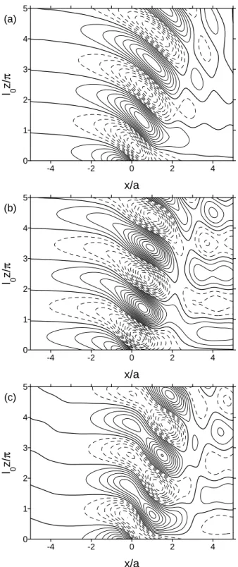
In Figure 4, the normalized vertical velocity pertur-bation w/(U h0/a) is shown in a vertical cross-section perpendicular to the ridge, as calculated from the analytical model for ε = 0.1, l0a = 5 and λa/U = 2 × 10−2. The three situations displayed in Figure 4(a), 4(b) and 4(c) are the same as those considered in Figure 3. Namely, in Figure 4(a) a non-resonant case with ε = 0 is considered. Figure 4(b) displays a case of drag enhancement with ε = 0.1,

n/l0= 2 and φ = 3π/2, while Figure 4(c) displays a case of drag attenuation with ε = 0.1, n/l0= 2 and φ = π/2. In all panels, the structure typical of propagating mountain waves can be seen, with elongated maxima and minima over the mountain, tilted upstream. Nonhydrostatic effects are visible, with some downstream propagation of the wave pattern and some attenuation as one moves upwards. In Figure 4)(a) (the non-resonant case) the negative lobe of the vertical velocity sitting directly above the ridge has a minimum value below -0.9, while in Figure 4(b) (the high-drag state) that minimum is lower than -1.3 and in Figure 4(c) (the low-drag state) the minimum is merely below -0.6. Obviously, these differences in magnitude of the vertical velocity explain the differences in the pressure perturbation described in the previous section. There are some additional

-4 -2 0 2 4

x/a

l

z

/

π

x/a

l

z

/

π

x/a

l

z

/

π

Figure 4. Normalized vertical velocity perturbation w/(U h0/a) as a function of normalized streamwise and vertical distance, from the analytical model for ε = 0.1, l0a = 5 and λa/U = 2 × 10−2. (a) Non-resonant flow (ε = 0), (b) drag enhancement (ε = 0.1 and φ = 3π/2), (c) drag attenuation (ε = 0.1 and φ = π/2). Solid contours: non-negative values, dashed contours: negative values. Contour spacing: 0.1.

differences. In Figure 4(b) the pressure perturbation extends somewhat more in the upstream and downstream directions than in Figure 4(a). In particular, the nonhydrostatic wake of the mountain waves is considerably enhanced. In Figure 4(c), on the other hand, the maxima and minima of the vertical velocity have a two-lobe structure.

-4 -2 0 2 4

x/a

l

z

/

π

x/a

l

z

/

π

x/a

l

z

/

π

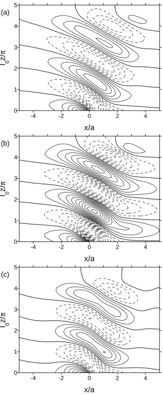
Figure 5. The same as Figure 4, but from the FLEX numerical model.

Figure 5 shows results similar to those of Figure 4, but produced by the FLEX numerical model. The minima of the vertical velocity perturbation above the ridge are just below -0.8 in Figure 5(a), below -1.2 in Figure 5(b) and below -0.6 in Figure 5(c). Concerning this aspect there is thus quite good agreement with Figure 4. However, the configuration of the flow shows some differences. For example, in Figure 5(b) the vertical velocity perturbation

extends less upstream of the ridge than in Figure 4(b), and the way in which it extends downstream is rather different. Differences are less marked between Figures 4(c) and 5(c), where the vertical velocity perturbation in the latter figure also displays a tendency for a two-lobe structure, although the nonhydrostatic wake is weaker than in Figure 4(c). Figures 4(a) and 5(a), where non-resonant conditions are considered, are perhaps the most similar, which is expectable, since they should correspond to the least nonlinear flow.

Unlike in Figure 4, in all panels of Figure 5 the flow perturbation tends to decay markedly above l0z/π = 4. This happens because the sponge applied in the numerical simulations at the top of the domain extends approximately down to that height. There is also more moderate attenuation below l0z/π = 4, which is clearly larger than in the analytical results, and a tendency for the flow pattern to become more horizontal. This could result from numerical dissipation associated with the discretization scheme. Either effect does not seem to have a large impact on the flow near the surface, as would be desirable for the present purposes.

It would be interesting to visualize the vertical velocity field given by the analytical model in invicid and resonant conditions. Unfortunately, for the same reasons as invoked for the pressure perturbation, the corresponding field diverges, and so is not presented here. The first-order term of this field, which is responsible for this divergence, does not display any tilting in its vertical structure (not shown), being therefore unable to increase the drag.

3.4. Nonhydrostatic effects

WV10 pointed out that, when the value of U is decreased, the drag maximum displayed in their Figure 9 for n/l0≈ 2 increased in magnitude. The present analytical model suggests that this behaviour may be explained by the variation of l0a, which increases as U decreases or as N0 increases. This motivates an exploration of the drag dependence on this parameter.

0.0 0.5 1.0 1.5 2.0 2.5 3.0 3.5 4.0 0.0 0.4 0.8 1.2 1.6 2.0 2.4 (a) D /D 0 n/l₀ 0.0 0.5 1.0 1.5 2.0 2.5 3.0 3.5 4.0 0.0 0.4 0.8 1.2 1.6 2.0 2.4 (b) D /D 0 n/l₀ 0.0 0.5 1.0 1.5 2.0 2.5 3.0 3.5 4.0 0.0 0.4 0.8 1.2 1.6 2.0 2.4 (c) D /D 0 n/l₀ 0.0 0.5 1.0 1.5 2.0 2.5 3.0 3.5 4.0 0.0 0.4 0.8 1.2 1.6 2.0 2.4 D /D 0 n/l₀ (d)

Figure 6. Normalized drag from (24) as a function of n/l0for ε = 0.1,

λa/U = 2 × 10−2_{and various values of l}

0a. Dashed line: l0a = 2, solid

line: l0a = 5, dotted line: l0a = 10. (a) φ = 0, (b) φ = π/2, (c) φ = π, (d) φ = 3π/2. 0.0 0.5 1.0 1.5 2.0 2.5 3.0 3.5 4.0 0.0 0.4 0.8 1.2 1.6 2.0 2.4 D /D 0 n/l 0 (a) 0.0 0.5 1.0 1.5 2.0 2.5 3.0 3.5 4.0 0.0 0.4 0.8 1.2 1.6 2.0 2.4 D /D 0 n/l 0 (b) 0.0 0.5 1.0 1.5 2.0 2.5 3.0 3.5 4.0 0.0 0.4 0.8 1.2 1.6 2.0 2.4 D /D 0 n/l 0 (c) 0.0 0.5 1.0 1.5 2.0 2.5 3.0 3.5 4.0 0.0 0.4 0.8 1.2 1.6 2.0 2.4 D /D 0 n/l 0 (d)

Figure 7. The same as Figure 6, but from the FLEX numerical model. Dashed line and squares: l0a = 2, solid line and circles: l0a = 5, dotted line and triangles: l0a = 10.

In Figure 6 the normalized drag predicted by (24) is presented as a function of n/l0 for ε = 0.1 and λa/U = 2 × 10−2_{, for the same values of φ as before and three}

values of l0a: 2, 5 and 10. It can be seen that the drag maxima and minima become more pronounced and narrower as l0a increases. For example, in Figure 6(d) the drag maximum has a magnitude of ≈ 2.6 when l0a = 10. This is still somewhat lower than the value of 3.5 predicted by (28) for perfectly hydrostatic conditions. By symmetry, this implies that, in Figure 6(b) the drag minimum is negative for l0a = 10, an unphysical result which stems for the limitations of the analytical model, as pointed out before. For l0a = 2, a case where the flow is highly nonhydrostatic, the minimum in Figure 6(b) and the maximum in Figure 6(d) are decreased, translated to slightly lower values of n/l0, and become wider on their left slopes. This should be caused by wave dispersion, which tends to ‘unfocus’ the resonance process. Since resonance relies on trapping by vertical reflections of the wave energy, dispersion attenuates it by allowing that energy to also propagate downstream instead of becoming only concentrated over the mountain.

Figure 7 shows similar results, but from the FLEX numerical model. Clearly, the main features in the drag variation with n/l0are in agreement with those of Figure 6, nevertheless because the drag is only plotted as a function of n/l0 at intervals of 0.25, some details are necessarily lost. For example, the increase in the magnitude of the drag extrema as l0a increases is less pronounced. This happens because, despite the fact that the drag minimum in Figure 7(b) and the drag maximum in Figure 7(d) become centred closer to n/l0(for which there is a computed value of D/D0), their width becomes smaller. Therefore, the magnitude of the drag extrema seems to be progressively more underestimated as l0a becomes larger. A similar phenomenon can be seen for the drag minimum in Figure 7(a) and 7(c) for l0a = 10. This implies that the drag extrema become more difficult to detect as the flow becomes more hydrostatic. There is an additional subtle difference

between Figures 6 and 7, whose cause is not clear. The drag to the left of the minimum in Figure 7(b) and to the left of the maximum in Figure 7(d) depart slightly more from 1 for l0a = 10 than for l0a = 5. Despite these differences, the behaviour of the analytical and of the numerical model clearly resemble each other qualitatively.

3.5. Numerical simulations with friction

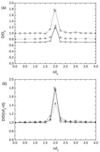
It was seen in the preceding sections that friction is a crucial effect for the type of resonance being addressed in this study, in particular for producing the single drag maximum (φ = 3π/2) or minimum (φ = π/2) at n/l0= 2. Since, among these two, the most relevant is undoubtedly the drag maximum, attention will be focused next on this case, with a preliminary analysis of the effect of physical friction (as opposed to numerical friction) on its behaviour. The following numerical results do not aim at more than illustrating how the drag variation is modified when a turbulence closure is adopted in the FLEX model, instead of running it in inviscid mode. A more comprehensive exploration of these effects is left for future studies.

Figure 8 reproduces the results from the FLEX numerical model for φ = 3π/2, ε = 0.1 and l0a = 5 also presented in Figure 2(d) (squares and dashed line). The circles and solid line correspond to the drag calculated with the same parameters, with the difference that a simple Smagorinsky-type turbulence closure, based on Lilly (1962), was turned on. For the triangles and dotted line, a K − ε turbulence closure was adopted instead. Clearly, by comparison with the inviscid drag, the presumably more realistic drag produced with the turbulence closures is somewhat reduced for all values of n/l0. For n/l06= 2 this reduction is larger using the Lilly closure than for the

K − ε closure. The level of the non-resonant drag in the

former case (≈ 0.7) is lower than that of the latter (≈ 0.8), which is comparable to that found in the viscous simulations of WV10. However, for n/l0= 2, the drag using both turbulence closures is comparable (≈ 1.2) and smaller than both the inviscid result and that shown in Figure 9 of WV10.

0.0 0.5 1.0 1.5 2.0 2.5 3.0 3.5 4.0 0.0 0.2 0.4 0.6 0.8 1.0 1.2 1.4 1.6 1.8 2.0 (a) D /D 0 n/l₀ 0.0 0.5 1.0 1.5 2.0 2.5 3.0 3.5 4.0 0.6 0.8 1.0 1.2 1.4 1.6 1.8 2.0 D /D (n /l0 = 0 ) n/l₀ (b)

Figure 8. Normalized drag as function of n/l0for ε = 0.1, l0a = 5 and φ = 3π/2 from the FLEX numerical model, in inviscid conditions (dashed lines and squares), using Lilly’s (1962) turbulence closure (solid lines and circles) and using a K − ε turbulence closure (dotted lines and triangles). (a) Same normalization as used previously (b) Drag normalized by its value at n/l0= 0.

If the drag is normalized, not by its inviscid non-resonant value, but by its value at the origin of n/l0 (which corresponds to the non-resonant viscous limit) (Figure 8(b)), it can be noticed that there are almost no differences between the inviscid result and that using the Lilly turbulence closure. This means that the drag is attenuated proportionally by friction in the latter case in all circumstances. Using the K − ε turbulence closure, on the contrary, the drag amplification is somewhat reduced compared with the inviscid simulations. This behaviour is also different from that displayed in Figure 9 of WV10, where a simple turbulence closure appears to have been used. Presumably, the K − ε turbulence closure, unlike the Lilly closure, becomes more active in resonant conditions, which makes some sense, since the flow is then more likely to become turbulent. The drag behaviour using the K − ε

turbulence closure could be mimicked using the present analytical model by increasing the value of λa/U , but, of course, the selected value would only be suitable for this particular case.

These results further emphasize the sensitivity of the drag to the representation of frictional effects, a finding which parallels those of previous authors for various types of resonant or high-drag orographic flows, for example

´

Olafsson and Bougeault (1997), Peng and Thompson (2003) and Stiperski and Grubiˇsi´c (2011). Clearly, in order to achieve a realistic representation of the drag in nature, particularly for the type of resonant flows being investigated here, much attention needs to be devoted to the formulation of turbulence closures in numerical models.

4. Concluding remarks

A mechanism of parametric resonance leading to the amplification of mountain waves, and their associated surface drag, was investigated, inspired by the recent study of WV10. This resonance relies on the existence of a vertically oscillating Scorer parameter, although this oscillation may be of relatively small amplitude. WV10 suggested that this mechanism is intrinsically nonlinear, being related with the wave-triad interaction originally addressed by Phillips (1968) in an oceanographic context. A linear model using a perturbation approach, where the solutions are expanded in powers of a small parameter proportional to the amplitude of the Scorer parameter oscillation was developed, showing that the wave and drag amplification mechanism under consideration is essentially linear, although it is obviously altered by nonlinearity when the drag is enhanced or attenuated by a large factor.

The results presented in the previous sections have substantial implications for numerical modelling of mountain waves. Since friction has a crucial impact on the magnitude, and even on the existence or not of drag maxima caused by the kind of parametric resonance being studied, a good representation of this process in numerical models appears to be essential to obtain accurate mountain wave

drag estimates. The behaviour of the drag should be quite sensitive to the particular turbulence closure employed, as is suggested by the preliminary viscous results presented in the preceding section. Inviscid calculations, on the other hand, are probably of limited quantitative value, since their resolution, or the degree of numerical diffusion associated with their particular discretization scheme, may alter substantially the way in which the resonance process is represented.

When comparing the results of the present study to those of WV10, some intriguing aspects were found. For example, on their page 436 these authors remark that the drag maxima produced by their numerical model corresponds to drag minima in their linear model. No such discrepancy in behaviour was ever found in the present calculations.

Instead of using (7) to define the Scorer parameter, WV10 added an expression of the form A sin(nz − φwv)

to the mean velocity U . At first glance, a simple relation between the perturbation imposed on the Scorer parameter by WV10 and that employed here could be described by

l2= N 2 0 {U + A sin(nz − φwv)}2 ≈ N 2 0 U2 ½ 1 + 2A U cos ³ nz − φwv+π 2 ´¾ , (29)

when A/U is small. Then, the small parameter used in the present study should be defined in terms of the quantities employed by WV10 as ε = 2A/U . However, the fact that in the present analytical model the oscillation in the Scorer parameter profile was implicitly imposed on N2 _rather than on U may lead to important differences in the results (Vosper, private communication). A possible explanation for this behaviour is that some of the integrals calculated in the solution procedure involve λa/U (see section 2.1), which would become a function of z instead of a constant if U oscillates in the vertical. This would considerably complicate the analytical treatment.

Several refinements and additions to the idealized situation considered here would be possible, and of substantial interest for mountain wave modelling. For example, 3D orography, which is obviously more realistic than a 2D ridge, could be adopted. This modification would be expected to weaken the resonance process, since it leads to a higher degree of wave dispersion (then not only associated with nonhydrostatic effects, but also with the variable orientation of the mountain waves).

A further step towards making the present model problem more realistic could be the prescription of Scorer parameter profiles with a more complicated form (i.e. containing more harmonics in the vertical). One of the motivations presented by WV10 for considering one single harmonic, as is done in the present study, results from their analysis of the spectrum of a more realistic Scorer parameter profile. Consideration of this effect would also, in principle, tend to weaken the resonance process under study, by spreading it over a wider range of n/l0than presently.

Finally, higher mountains, for which N0h0/U is closer to unity, and hence where the flow becomes nonlinear even in the absence of resonance, could be considered. Clearly, this more realistic situation could only be investigated using a set of numerical simulations. This, as well as the other developments alluded to above, are left as suggestions for future work.

Acknowledgement

We are grateful to Dr. Simon Vosper and an anony-mous referee for insightful comments, which have sig-nificantly improved this paper. The present work was supported by Fundac¸˜ao para a Ciˆencia e Tecnologia (FCT) under Projects PEst-OE/CTE/LA0019/2011-IDL and PTDC/EME-MFE/099636/2008.

Appendix A. The vertical wavenumber of the waves

Using (13), (12) may be decomposed into its real and imaginary parts, yielding the following two equations:

m2 I− m2R− 2 λ U kmRmI+ l 2 0− k2 = 0, (A1) 2mRmI + λ U k(m 2 I− m2R) − λk U = 0. (A2)

If (A1) and (A2) are combined, a single equation for mIcan

be found: m4 I+ Ã l2 0 1 + λ2 U2_k2 − k2 ! m2 I− 1 4 λ2 U2_k2 l4 0 ¡ 1 + λ2 U2_k2 ¢2 = 0. (A3) In order to calculate mI, (A3) must be solved for m2I and

then the positive root for mI must be selected. Combining

(A1)-(A2) in an alternative way, a relationship that gives

mRin terms of mI is obtained: mR= λ U kl02 2mI ¡ 1 + λ2 U2_k2 ¢ . (A4)

It can be seen from (A4) that if mI > 0, then mR has the

same sign as U k, which automatically satisfies the radiation boundary condition. The mIfound as a solution to (A3) and

the corresponding mRcalculated from (A4) are presented in

(14) and (15).

Appendix B. The first-order wave solution

The most general solution to (10) is of the form:

ˆ w1= a eimz+ b e−imz− 1 2im l2 0 1 − i λ U k × Z _z 0 ˆ w0cos(ns + φ) n eim(z−s)− e−im(z−s) o ds, (B1)

where a and b are coefficients determined by the boundary conditions. The boundary conditions that ˆw1(z = 0) = 0 and that ˆw1 remains finite as z → +∞ are only satisfied

if a = −b = 1 2im l2 0 1 − i λ U k Z _+∞ 0 ˆ

w0cos(nz + φ)eimsds. (B2) Then (B1) can be written:

ˆ w1= 1 2im l2 0 1 − i λ U k ·Z _+∞ 0 ˆ

w0cos(ns + φ)eimsds סeimz_{− e}−imz¢₋ Z z 0 ˆ w0cos(ns + φ) × n eim(z−s)− e−im(z−s) o ds i . (B3)

Using (11) in (B3), (16) is readily obtained.

Appendix C. The pressure perturbation

If (8) and (20) are used in (19), and this latter equation is evaluated at z = 0, the zeroth-order pressure perturbation is given by ˆ p0(z = 0) = iρ0 k {U 0 0wˆ0(z = 0) −U0 µ 1 − i λ U k ¶ ˆ w00(z = 0) ¾ . (C1)

Inserting (11) into (C1), it is easy to show that

ˆ p0(z = 0) = ρ0U0ˆh ½ iU0m µ 1 − i λ U k ¶ − U00 ¾ . (C2)

Using additionally (13), (21) is straightforwardly obtained. Using (8) and (20) in (19), the first-order pressure perturbation at z = 0 is given by ˆ p1(z = 0) = −iρ0U0 k µ 1 − i λ U0k ¶ ˆ w0 1(z = 0), (C3)

where the fact that ˆw1(z = 0) = 0 has been noted. If (17) is differentiated with respect to z and evaluated at z = 0, the result is: ˆ w0 1(z = 0) = U0kˆh l 2 0 1 − i_{U k}λ 1 4m2_{− n}2(in sin φ −2m cos φ). (C4)

If this equation is inserted into (C3), and (13) is also employed, (22) is obtained after some algebra.

References

Abramowitz M, Stegun IA. 1972. Handbook of Mathematical

Functions: with Formulas, Graphs, and Mathematical Tables. Dover

Publications, Inc.

Arga´ın JL, Miranda PMA, Teixeira MAC. 2009. Estimation of the friction velocity in stably stratified boundary-layer flows over hills.

Boundary-Layer Meteorol. 130: 15–28.

Grisogono B, Pryor SC, Keislar, RE. 1993. Mountain wave drag over double bell-shaped orography. Q. J. R. Meterol. Soc. 119: 199–206. Grubiˇsi´c V, Stiperski I. 2009. Lee-wave resonances over double

bell-shaped obstacles. J. Atmos. Sci. 66: 1205–1228.

Lee Y, Muraki DJ, Alexander DE. 2006. A resonant instability of steady mountain waves. J. Fluid Mech. 568: 303–327.

Leutbecher M. 2001. Surface pressure drag for hydrostatic two-layer flow over axisymmetric mountains. J. Atmos. Sci. 58: 797–807. Lilly DK. 1962. On the numerical simulation of buoyant convection.

Tellus 14: 148–156.

Lin Y-L. 2007. Mesoscale Dynamics. Cambridge University Press. Miranda PMA, Valente MA. 1997. Critical level resonance in

three-dimensional flow past isolated mountains. J. Atmos. Sci. 54: 1574– 1588.

Nance LB, Durran D. 1998. A modeling study of nonstationary trapped mountain lee waves. Part II: nonlinearity. J. Atmos. Sci. 55: 1429– 1445.

´

Olafsson H, Bougeault P. 1997. The effect of rotation and surface friction on orographic drag. J. Atmos. Sci. 54: 193–210.

Peng M, Thompson WT. 2003. Some aspects of the effect of surface friction on flows over mountains. Q. J. R. Meteorol. Soc. 129: 2527– 2557.

Phillips OM. 1968. The interaction trapping of internal gravity waves.

J. Fluid Mech. 34: 407–416.

Queney P. 1948. The problem of airflow over mountains: A summary of theoretical studies. Bull. Am. Meterol. Soc. 29: 16–26.

Stiperski I, Grubiˇsi´c V. 2011. Trapped lee wave interference in presence of surface friction. J. Atmos. Sci., in press.

Teixeira MAC, Miranda, PMA. 2004. The effect of wind shear and curvature on the gravity wave drag produced by a ridge. J. Atmos.

Sci. 61: 2638–2643.

Teixeira MAC, Miranda PMA. 2005. Linear criteria for gravity wave breaking in resonant stratified flow over a ridge. Q. J. R. Meterol.

Soc. 131: 1815–1820.

Teixeira MAC, Miranda PMA. 2006. A linear model of gravity wave drag for hydrostatic sheared flow over elliptical mountains. Q. J. R.

Meteorol. Soc. 132: 2439–2458.

Teixeira MAC, Miranda PMA, Arga´ın, JL. 2005. Resonant gravity wave drag enhancement in linear stratified flow over mountains. Q. J. R.

Meteorol. Soc. 131: 1795–1814.

Teixeira MAC, Miranda PMA, Arga´ın, JL. 2008. Mountain waves in two-layer sheared flows: critical level effects, wave reflection and drag enhancement. J. Atmos. Sci. 65: 1912–1926.

Vosper S. 1996. Gravity-wave drag on two mountains. Q. J. R. Meteorol.

Soc. 22: 993–999.

Wang, T-A, Lin Y-L. 1999. Wave ducting in a stratified shear flow over a two-dimensional mountain. Part I: General linear criteria. J. Atmos.

Sci. 56: 412–436.

Wells H, Vosper SB. 2010. The accuracy of linear theory for predicting mountain-wave drag: Implications for parametrization schemes. Q. J.