Decomposing and analysing the determinants of current accounts’ cyclicality : evidence from the Euro Area

(1)

REM WORKING PAPER SERIES

DECOMPOSING AND ANALYSING THE DETERMINANTS OF

CURRENT ACCOUNTS’ CYCLICALITY: EVIDENCE FROM THE

EURO AREA

António Afonso, João Jalles

REM Working Paper 042-2018

June 2018

REM – Research in Economics and Mathematics

Rua Miguel Lúpi 20,

1249-078 Lisboa, Portugal

ISSN 2184-108X

Any opinions expressed are those of the authors and not those of REM. Short, up to two paragraphs can be cited provided that full credit is given to the authors.

(2)

D

ECOMPOSING AND

A

NALYSING THE

D

ETERMINANTS OF

C

URRENT

A

CCOUNTS

’

C

YCLICALITY

:

E

VIDENCE FROM THE

E

URO

A

REA

*

António Afonso

$

_{João Tovar Jalles}

#

April 2018

Abstract

In this paper, we decompose the current account (CA) balance in 19 Euro area countries into cyclical and non-cyclical components. For the period 1999:Q1 to 2015:Q4, we compute income elasticities of imports and of exports via an alternative novel and improved approach by running time-varying coefficient models country-by-country. Then, in a panel set-up (and controlling for country-invariant characteristics), we uncover that terms of trade have a positive effect on both the cyclical and non-cyclical components of the CA, while the Global Financial Crisis, compensation of employees and the employment level have a negative effect on the cyclical component. Moreover, the crisis had a greater impact on the cyclical component of the CA due to movements in the real effective exchange rate. In addition, we find a negative effect of the crisis on the cyclical component of the CA for countries that received financial assistance from the European Union, notably Ireland, Portugal, Spain and Latvia.

JEL: C23; F32; G01

Keywords: current account cyclicality; financial markets; time-varying coefficients

*_{We thank two anonymous referees for useful comments and suggestions in an earlier version of the paper. Thanks also}

go to Luis Catão for useful comments. Any remaining errors are ours alone. The opinions expressed herein are those of the authors and do not reflect those of their employers.

$_{ISEG/UL - Universidade de Lisboa, Department of Economics; REM – Research in Economics and Mathematics, UECE}

– Research Unit on Complexity and Economics. UECE is supported by FCT (Fundação para a Ciência e a Tecnologia, Portugal). email: [email protected].

#_{Centre for Globalization and Governance, Nova School of Business and Economics, Campus Campolide, Lisbon,}

(3)

2

1. Introduction

The assessment of the cyclicality of the current account (henceforth CA) balances is an issue of relevance notably for the sake of its macroeconomic effects in today’s growingly integrated world. In fact, one can think of the need to reach or maintaining a certain level of current balances in order to stabilise the net foreign asset position of a given country. Moreover, the potential determinants of the CA dynamics might differ if one considers the cyclical component of the CA or, alternatively, its non-cyclical component.

In this context, the European Commission’s Macroeconomic Imbalance Procedure uses an alert mechanism based on a scoreboard of headlines indicators with indicative thresholds that intend to cover potential sources of macroeconomic imbalances. The CA imbalance is one of those indicators, assessed via a 3-year backward moving average of the CA balance (in percent of GDP), with upper and lower margins of +6 percent and -4 percent. Hence, the study of CA cyclicality has important implications notably for the sustainability of the CA deficit. Indeed, concerns frequently arise about a widening CA deficit and corrective measures required to address it.

Against this background, it is important to have measures of income elasticities of exports and imports, for each country in our panel. Since trade shares change throughout time and across countries, it is crucial to recognize that the aforementioned elasticities might not be time invariant, and, hence, one should allow for time-varying elasticities, Hence, we use a time-varying coefficient set-up to explanation cross‐ and within‐country variation in the cyclical and non-cyclical CA components, which is to the literature. In practice: i) we decompose the CA into cyclical and non-cyclical components for a sample of 19 Euro area countries between 1999:Q1 and 2015:Q4; ii) we compute income elasticities of imports and of exports via an alternative novel and improved approach, employing country-specific time-varying coefficient models; iii) we control for country-invariant controls via a panel setup.

Our work in this paper is important as it provides a refinement of current account’s components which is not only relevant from a policy perspective, but also provides a useful countercheck of the relatively simply methodologies sometimes employed when conducting policy decisions. Moreover, compared to the many papers inspecting current account drivers (refer to section 2 for a review), the main value added of our approach lies in discriminating variables that affect the cyclical position only. From a pure academic perspective, this paper can thus help to distinguish between cyclical and non-cyclical current account drivers.

(4)

3

We find that terms of trade have a positive effect on both the cyclical and non-cyclical components of the CA, while the 2008-2009 Global Financial Crisis (henceforth GFC), compensation of employees and the employment level have a negative. Moreover, the crisis had a greater impact on the cyclical component of the CA due to movements in the real effective exchange rate. In addition, we find a negative effect of the crisis on the cyclical component of the CA for countries that received financial assistance from the European Union, notably Ireland, Portugal, Spain and Latvia.

The remainder of the paper is organized as follows. Section 2 briefly reviews the literature. Section 3 outlines the empirical methodology. Section 4 presents and discusses the main empirical results. The last section concludes and elaborates on policy implications.

2. Literature

Several papers studied the relevance of CA imbalances, stemming notably from the standalone CA determinants to the twin-deficit issue. The question is quite topical for the Euro area context where a usual determinant of CA imbalances, the exchange rate, is locked in a common currency.

Chinn and Hiro (2007) use annual data for 89 industrial and 70 developing countries covering the period 1971-2004, and mention notably that developed financial markets would lead to smaller current account balances for countries with highly developed legal systems and open financial markets. Additionally, increases in the budget balance would also improve the current account balance.

Lane and Milesi-Ferretti (2012) looking at a panel of 65 countries, report that CA imbalances until 2008 were explained by rising oil prices, credit booms and asset price bubbles, and easy external financing conditions. In the case of countries with pre-crisis CA balances in “excess deficit” deviation, there was evidence of large contractions in their external accounts, while the real exchange rate was a destabilizing (stabilizing) factor across pegged (non-pegged) currencies. Moreover, the external assistance and European Central Bank (henceforth ECB) liquidity softened the outflow of private capital from the euro area deficit countries.

Chen et al. (2013) argued that the international trade path of the decade 1999-2008 was favourable to core Euro area countries contrary to European deficit ridden countries. Investors from the rest of the world favoured purchasing financial instruments issued by countries such as Germany and France.

(5)

4

Guillemette and Turner (2013) assess the building up of current account imbalances for 12 euro area countries with a SUR (Seemingly Unrelated Regression) approach using data for the period 1998 to 2011. They report that a key determinant of current account balances is the change in competitiveness, notably for the cases of the euro area so-called periphery economies, while the main adjustment in the current account imbalances since the GFC is deemed to have occurred on the cyclically adjusted component.

In an analysis for the United States, the Euro area, Japan and China, Ollivaud and Schwellnus (2013), for the period 1996-2012, mention that business and housing cycles have accounted for half of the decrease in international imbalances. Hence, the improvement in current account balances is due to the respective cyclical component.

Phillips et al. (2013) estimate CA residuals for a set of 49 advanced and emerging market economies, with annual data, for the period 1986-2010. According to the authors, the REER plays a key role together with some non-policy variables (for instance, expected real growth) and cyclical factors (for instance, terms of trade).

In a related strand of research, Cheung et al. (2013) assess the links between non-cyclical and cyclical factors and CA balances in a panel of 94 countries from 1973 to 2008. The authors report that structural, non-cyclical, factors such as fiscal deficits, oil dependency, economic development, financial market development, and institutional quality explain CA balances.

Hobza and Zeugner (2014) employed a dataset of bilateral financial stocks and flows among Euro area countries in the period 2001-2012, and concluded that CA deficits of the euro area periphery countries were almost exclusively financed from the rest of the zone. In fact, France became the main financing country in 2009 of deficit countries after the withdrawn of funding from surplus countries, mainly Germany. However, during the period 2004-2006 there were outflows from Germany and the Benelux to the periphery.

More country specific studies were performed notably by Kollmann et al. (2015), who studied German’s CA during the period 1995-2015, and Afonso and Silva (2017) who assessed the cyclicality of CA balances for the period 2001Q1-2014Q4, focussing on Portugal and Germany. Kollmann et al. (2015) reported that the German CA surplus reflected a positive impact to the German saving rate due to changes in the retirement system; demand for German exports by the rest of the world; German labour market reforms via unemployment benefit cuts; and other aggregate supply shocks such as total factor productivity.

(6)

5

On the other hand, Afonso and Silva (2017) found that the cyclical component of the current account was positively explained by 3-months Euribor, but negatively by the financial crisis, systemic stress in Europe, employment and compensation of employees. Moreover, the non-cyclical current account was positively affected by the period of the Economic and Financial Adjustment Program and the terms of trade, but negatively influenced by financial integration.

In addition, one would expect a positive effect for the non-cyclical component of the CA following some structural reforms in periphery EU countries, after the Global Financial crisis. Therefore, after the closing of the output gap in those countries, eventual CA imbalances would be more mitigated than the ones from the period 2000-2007 (see Catão, 2017).

3. Methodology

In our empirical analysis, we start by following the decomposition of the current account-to-GDP ratio (into cyclical and non-cyclical elements) used by Salto and Turrini (2010) and by the European Commission (2014).1_{Equation (1) lays out the impact of national and foreign output gaps as well as}

the effect of the real exchange rate on the non-cyclical (underlying) current account balance, ݑܿܽ_௜௧:2

ݑܿܽ௜௧ =_ܲܥܣ௜௧ ௜௧ܻ௜௧+ ߠெ ܲ௜௧ெܯ௜௧ ܲ௜௧ܻ௜௧ ∗ ܻ௜௧− ܻ௜௧∗ ܻ_௜௧∗ − ߠ௫ܲ௜௧ ௑_ܺ ௜௧ ܲ௜௧ܻ௜௧ ∗ ܻ௜௧ி− ܻ௜௧ி∗ ܻ_௜௧ி∗ + + ൬௉೔೟೉௑೔೟ ௉೔೟௒೔೟ߟ௫− ௉_೔೟ಾெ೔೟ ௉೔೟௒೔೟ ߟெ൰ ሺ0.4 ∗ ∆ݎ݁݁ݎ௜௧+ 0.15 ∗ ∆ݎ݁݁ݎ௜௧ିଵሻ. (1)

where ܥܣ_௜௧ is the nominal current account of goods and services, ܲ_௜௧ܻ_௜௧ denotes nominal GDP, and ܲ_௜௧ெ_ܯ

௜௧ and ܲ௜௧௑ܺ௜௧ are nominal imports and exports of goods and services, respectively. Additionally,

M

θ and θ_X are the income elasticity of imports and exports, reerit is the real effective exchange rate,

X

η and η_Mdenote the elasticities of exports and imports with respect to the real effective exchange

1_{The analysis also builds on the IMF inter-temporal approach to the current account (see among others Lee and al. (2008),}

Christiansen et al. (2009) and Phillips et al. (2013)) to assess how much the improvement could be explained by permanent non-cyclical changes.

2_{We assume that the output gap of the trading partner is the Euro area as a whole. For instance, Wierts et al. (2012)}

mention that around 1/3 of the exports of the euro area were in 2008 to the euro area itself. Regarding the use of the output gap in related analysis, Philipps et al. (2013) in the context of the IMF External Balance Assessment methodology, use the world GDP-weighted average output gap. On the other hand, Salto and Turrini (2010) to compute the foreign output gap they use the output gap of the 40 competitor countries weighed by the bilateral trade shares.

(7)

6 rate (REER).3 _it

it

Y

−

* and YFit −YF*it are national and foreign output gaps (with superscript * denoting potential output4_{), respectively.}

However, and contrarily to Salto and Turrini (2010) and European Commission (2014), instead of assuming constant elasticities and equal to all countries5_{, we propose an alternative novel and}

improved approach. This consists of estimating time-varying elasticities country-by-country.6_Not

only does this mimic better the true behaviour of elasticities over time, but it also accounts for cross-country heterogeneity by estimating these elasticities on a cross-country-by-cross-country basis. An elasticity can be estimated on a log-log equation representation of the following form:

ܼ௜ = ߙ௜ + ߚ௜ܭ௜ + ߝ௜ (2)

where ܼ_௜ is either the log of imports or the log exports (with subscripts M or X, respectively); ܭ_௜ is either the log of output (in the case of the estimation of θMand θX) or the log of the REER (in the case of the estimation of η_X and η_M). In order to have time-varying estimates of our elasticity parameter ߚ_௜ , we generalize equation (2) by introducing the assumption that the regression coefficients may vary over time:

ܼ௜ = ߙ௜௧+ ߚ௜௧ܭ௜+ ߝ௜ (3)

where the coefficient ߚ_௜௧ is now assumed to change slowly and unsystematically over time and that the expected value of the coefficient at time t is equal to the value of the coefficient in time t-1 (i.e. the coefficient is assumed to be a random walk). The change of the coefficient is given by ݒ_௜,௧, which is assumed to be normally distributed with expectation zero and variance ߪ_௜ଶ:

3_{Faruquee and Debelle (2000) have observed that a country’s position in the business cycle, as measured by the output}

gap and the real exchange rate, had significant short-term effects on the current account balance for a number of industrial countries during the 1971-93 period.

4_{Potential output is retrieved from the AMECO database. For further details on sources and definitions refer to Table A0}

in the Appendix.

5_{Salto and Turrini (2010) refer that usually income elasticity of exports and imports are 1.5 and 1.5, respectively. In}

addition, the elasticities of exports and imports with respect to the REER has been suggested to equal -1.5 and 1.25, respectively.

6_{Note that endogeneity could be potentially an issue when estimating country-specific elasticities. However, the}

time-varying model employed does not allow for an instrumental-variable approach. Moreover, finding country-specific suitable instruments for each type of elasticity (so as to avoid using several lags and, hence, reduce further the degrees of freedom available) goes beyond the scope of this paper. We thank an anonymous referee for this point.

(8)

7

ߚ௜௧= ߚ௜௧ିଵ+ ݒ௜௧. (4)

Equations (3) and (4) are jointly estimated using the Varying-Coefficient Model proposed by Schlicht (1985, 1988). Here, the variances ߪ_௜ଶ are computed using a method-of-moments estimator, which coincides with the maximum-likelihood estimator for large samples (see Schlicht, 1985, 1988 for details). The model described in equations (3) and (4) generalizes the classical regression model (equation 2), which is obtained as a special case when the variance of the disturbances in the coefficients approaches to zero.

This approach has multiple advantages compared to other approaches used to compute time-varying coefficients such as rolling windows and Gaussian methods (Aghion and Marinescu, 2008). First, it allows using all observations in the sample to estimate the degree of responsiveness of each determinant in each year – a construction not possible in the rolling windows method. Second, changes in the elasticity in a given year come from innovations in the same year, rather than from shocks occurring in neighbouring years. Third, it minimizes reverse causality problems when the estimated elasticities are employed as explanatory variables since they depend on the past.

Equation (1) can be re-written in econometric form as being determined by a combination of domestic and foreign factors. For it one can derive the cyclical component of the CA simply as the difference between CA and its non-cyclical component. The cyclical component of the CA is the CA that would prevail if all economies in the world were at potential and exchange rates were stable. More specifically, we have:

'

D

'

F it it it it

uca

= +

α β

P

+

δ

Q

+

v

₍₅₎

/

'

D

'

F it it it it it it it it

ca CA PY uca a b P

=

−

= +

+

d Q

+

e

(6) where PDit and it F

Q

are vectors of domestic and foreign regressors, respectively.

v

it and

e

itare

white-noise disturbance terms satisfying usual assumptions of zero mean and constant variance. According to economic theory, some key fundamentals can be tested as determinants of cyclical and non-cyclical CA movements. We include the following sets of domestic and foreign explanatory variables:7

7_{Our approach builds on existing literature notably Kraay and Ventura (2002), Chinn and Prasad (2003),}_{Lee and al.}

(9)

8

• Financial volatility: composite indicator of systemic stress (CISS) and a measure of financial stress in Europe and volatility index (VIX) as a proxy for global financial volatility.

• Financial fragmentation/integration: the share of monetary financial institutions cross-border holdings of the Euro area sovereign debt securities (cross-border holdings).

• Domestic factors: terms of trade, total employment, household’s disposable income (percent of GDP) and compensation of employees.

Moreover, we also make use of country-invariant control variables related to the interest rates (Euribor 3 months) and financial markets (SP 500 index). A dummy for the GFC is added to assess its impact on the cyclicality of CA balances (the dummy takes the value one starting in 2009:Q1). Freund (2000) found that the CA balances of most industrial countries depends on the economy’s position in the business cycle, with deficits typically widening during the expansionary phase of a business cycle and contracting or becoming surpluses as real GDP growth declines. This is because investment and imports are likely to increase during an economic boom.8_{Thus, we would expect real}

growth to have a negative impact on the current account balance, raising imports of goods and services. Finally, we estimate by Ordinary Least Squares our specifications (5) and (6) in first differences to circumvent the non-stationarity properties of the dependent variables.9 10

4. Empirical Analysis

4.1. Current Account cyclical and non-cyclical components

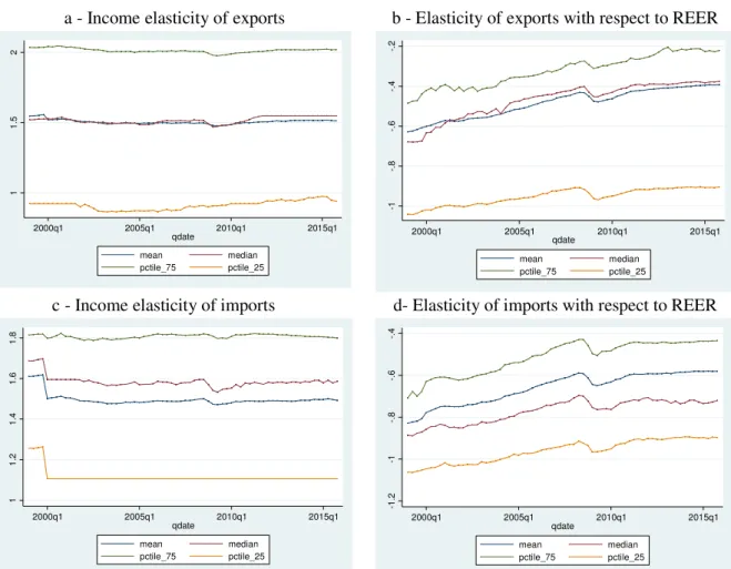
We decompose the CA into the cyclical and the non-cyclical components for each of our 19 Euro area countries using quarterly data for the period 1999:Q1 to 2015:Q4 (all data are described in the Appendix). Results of the estimation of the time-varying coefficient models of both the income elasticities of exports and imports, and of the REER elasticities of exports and imports are illustrated in Figure 1. In the case of the export and import elasticities vis-à-vis the REER an upward trend is

8_{The cyclicality of domestic investment relative to national savings is crucial to determine the cyclicality of the current}

account balance. In countries where domestic savings are low, boom periods do not result in a significant increase in savings. Other components of national savings, namely net foreign income and current transfers, are likely to be less dependent on domestic cyclical conditions. Hence, the cyclicality of domestic investment is likely to be more dominant in determining cyclical fluctuations in the current account balance than net foreign income and current transfers.

9_{For reasons of parsimony, unit root tests for our dependent variables are available from the authors upon request.} 10_{Note that when the computation of uca depends on time-varying elasticities, equations (5) and (6) are estimated using}

a Weighted Least Squares estimator to control for uncertainty related to the estimated coefficients. The weights are given by the inverse of the standard deviation of the estimated time-varying coefficient estimates.

(10)

9

visible for the entire panel. On the other hand, in the case of export and import elasticities vis-à-vis income the time profile of the entire panel does not suggest much upward or downward movement.

[Figure 1]

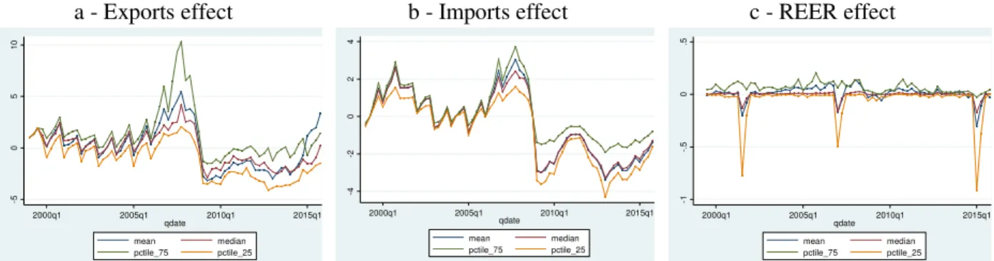
Figure 2 presents the cyclical and the non-cyclical components of the CA for the entire period under scrutiny. In the case of the cyclical component, it is possible to observe a decrease roughly after 2010, which can be related to some extent to the 2009 European debt crisis. An opposite increasing trend is depicted for the case of the non-cyclical component of the CA. In fact, the contributions of exports and imports to the cyclical component of the CA have declined sharply after the 2009 European debt crisis (Figure 3), implying a higher responsiveness to the business cycle of these components.

[Figure 2] [Figure 3]

4.2. Determinants of cyclical and non-cyclical components of the Current Account

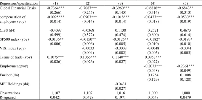
As far as the determinants of the cyclical component of the CA are concerned, Table 1 shows that terms of trade have a positive effect, while the global financial crisis, the compensation of employees and the employment level all have a negative impact.11_{In addition, financial instability (as}

proxied by the SP500 composite index) also had a negative impact on the cyclical component of the CA.

[Table 1]

Turning to the determinants of the non-cyclical component of the CA, we can observe from Table 2, that the y-o-y change of the terms of trade had an upward impact (as mentioned for instance by Guillemette and Turner, 2011), together with the dummy denoting the global financial crisis. In this latter case, we find support that the crisis had a greater impact on the non-cyclical component of the CA, as previously illustrated in Figure 1 with the structural level shift in exports and imports

11_{Kraay and Ventura (2002) show the impact of income fluctuations on the current account. Countries smooth their}

consumption by raising savings when income is high and vice versa. In the short-run, countries invest most of their savings in foreign assets. Fluctuations in savings lead to fluctuations in the current account that are equal to savings times the share of foreign assets in the country portfolio. The ability to purchase and sell foreign assets allows countries not only to smooth their consumption, but also their investment. Foreign assets and the current account absorb part of the volatility of these other macroeconomic aggregates.

(11)

10

elasticities due to movements in the REER (a factor whose relevance was previously highlighted by Lane and Milesi-Ferretti, 2012, and Philips et al., 2013). Hence, while the GFC reduced the cyclical component of the CA it increased the non-cyclical component of the CA (following up also the findings of Cheung et al., 2013).

[Table 2]

We also split the sample and took the EU12 and remainder of the countries in our dataset separately. Re-estimating specifications (4) and (5), show that for the cyclical component of the CA, the compensation of employees still has a negative and significant impact notably in the case of the non-EU12 countries.12_{However, now the change in the Euribor comes out statistically significant,}

increasing (decreasing) the cyclical part of the CA in the case of EU12 (non-EU12) countries. In the case of the non-cyclical part of the CA, the positive effect of the terms of trade, picked before for the full panel, remains statistically significant only in the case of the non-EU sub-sample. In addition, a higher Euribor was found to lower the non-cyclical part of the CA for the EU12 countries.

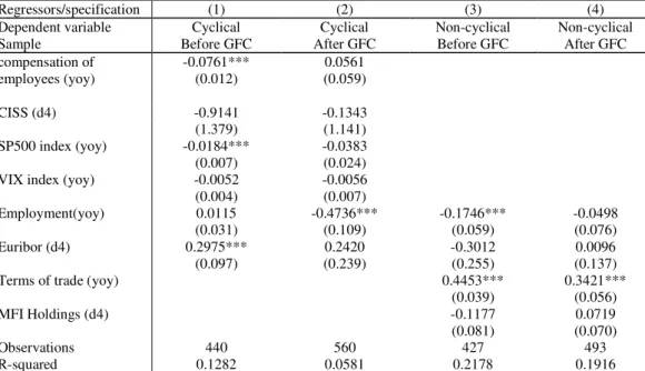
Since, as observed in both Tables 1 and 2, the effect of the GFC (starting in 2009:Q1) seems to matter in explaining movements of both cyclical and noncyclical CA balances, we split the time span into two non-overlapping periods: one before the start of the GFC and one after. We re-estimate equations (5) and (6) and the new results are displayed in Table 3. In fact, the two sub-periods depict some interesting differences, notably regarding the cyclical component of the CA: while before the GFC capital market related drivers (such as the Euribor and stock market returns (SP500)) where statistically relevant, ex-post they no longer matter. On the other hand, the employment level decreases the cyclical component, as in the full sample, but only after the GFC.

[Table 3]

Different countries have different time profiles in their cyclical and non-cyclical components of the current account, as confirmed by Figures A2.a and A2.b in the Appendix. For instance, one observes a positive development of the non-cyclical component of the CA in periphery EU countries (Greece, Portugal, Ireland, and Spain) after the GFC. Moreover, as suggested by Afonso and Silva (2017) the determinants affecting, for instance, Portugal’s CA cyclicality are different from those

(12)

11

affecting Germany’s. Henceforth, since we are relying on quarterly frequency data, we can run our main regressions country-by-country, which is yet another benefit of our analysis. Nonetheless, caution is needed when interpreting the results of some countries as the total number of observations varies raising potential issues related to “near-micronumerocity”.13_{Our country-specific results are}

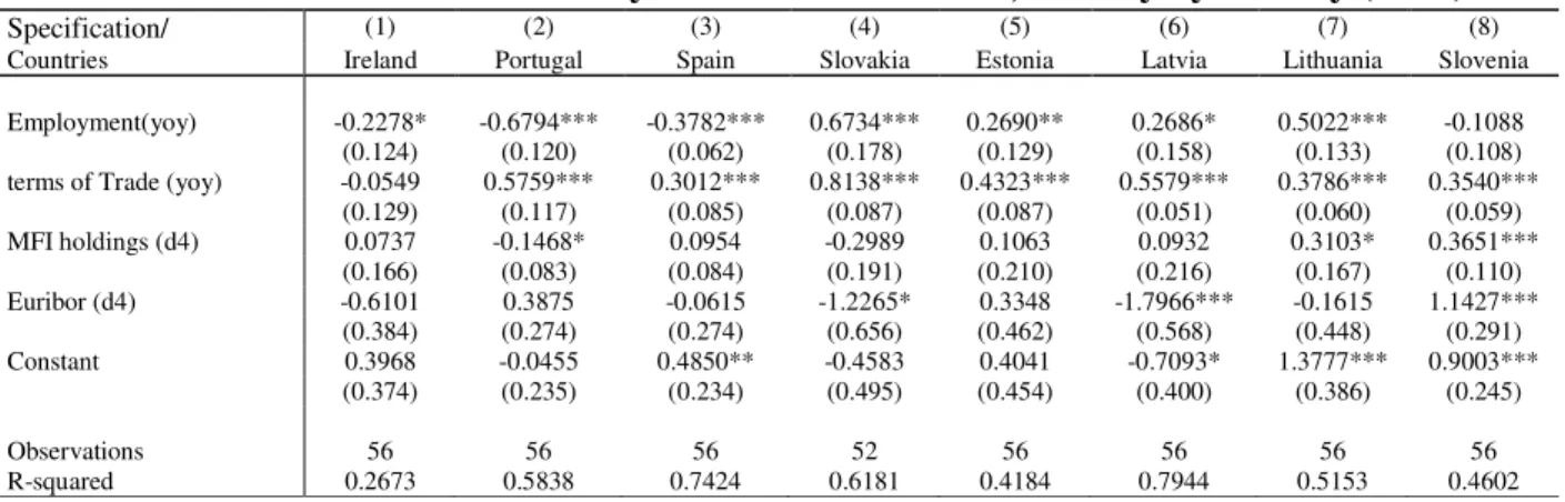
displayed in Tables A2-A3 in the Appendix. Regarding the main determinants of the cyclical component of the CA (Table A2), the negative effect of the compensation of employees is confirmed in 11 countries (out of 19) in the sample. Interestingly, it is also possible to observe the negative effect of the crisis on the cyclical component of the CA for the cases of Italy, Ireland, Portugal, Spain and Latvia. Interestingly, the latter four countries have received financial assistance from the European Union via financial mechanisms, which provided loans conditional on the implementation of policies designed to address underlying economic problems. On the other hand, Table A3 provides the estimated effects of the main determinants of the non-cyclical component of the CA. In this case, the positive statistical relevance of the terms of trade is worthwhile mentioning (for 9 countries out of 19).

4.3. Sensitivity analysis

We have also implemented a sensitivity analysis regarding the dependent variable, in order to assess to what extent our results are dependent on the weights used for the contemporaneous and lagged change in REER. More specifically, since the construction of the non-cyclical current account component lies on some assumptions regarding elasticities and the contemporaneous and lagged effect of changes in the REER, we postulate five alternative specifications to test the robustness of our results, as follows:

Alternative specification 1: this approach follows exactly the approach presented by Afonso and Silva (2017) in assuming fixed elasticities (cf. footnote 5) and the same weights of 0.4 and 0.15 for the contemporaneous and lagged change in REER.

Alternative specification 2: this approach also assumes fixed elasticities (cf. footnote 5) and slightly larger weights of 0.5 and 0.2 for the contemporaneous and lagged change in REER.

Alternative specification 3: this approach also assumes fixed elasticities (cf. footnote 5) and slightly smaller weights of 0.3 and 0.1 for the contemporaneous and lagged change in REER.

(13)

12

Alternative specification 4: this approach also assumes fixed elasticities (cf. footnote 5) and weights of 0.4, 0.2 and 0.1 for the contemporaneous, lagged and twice-lagged change in REER. Hence, a stronger effect of serial correlation is allowed for.

Alternative specification 5: this approach also assumes time-varying elasticities and the baseline weights of 0.4 and 0.15 for the contemporaneous and lagged change in REER. The difference here is that the foreign economy instead of being the Euro Area as a whole, corresponds to each country’s trading partners’ real GDP (see notably Salto and Turrini, 2010, as mentioned before). Using this information then the Hodrick-Prescott (HP) filter is applied to get both the output gap and the potential GDP (at the quarterly frequency). The newly computed output gap

(

Y

Fit

−

Y

F*it

)

new is then divided

by the new foreign potential GDP (whose weight is country specific).

The correlation coefficients between our baseline measure and the ones coming out of the 5 hypotheses described above are presented in Table A1 in the Appendix. We observe that the correlations and generally very high, which reassure us regarding the robustness of our (baseline) findings. That said, the re-estimation of equations (5) and (6) under the five alternative specifications for the dependent variables, yields the output in Table 4. In fact, the results remain qualitatively unchanged.

[Table 4]

5. Conclusion

In this paper, we have contributed to the rather scarce literature of assessing the determinants of current account cyclicality in several ways. First, we have decomposed the current account balance into cyclical and non-cyclical components for 19 euro area countries between 1999:Q1 and 2015:Q4. Second, we have computed the income elasticities of imports and of exports via an alternative novel and improved approach by estimating time-varying elasticities on a country-by-country basis. Third, we have explored the determinants of current account cyclicality in a panel setting controlling for country-invariant characteristics.

Our results show that: i) terms of trade have a positive effect on both the cyclical and non-cyclical components of the CA, while the GFC, compensation of employees and the employment level have a negative effect on the cyclical component; ii) the terms of trade and the GFC had an upward impact on the non-cyclical component of the CA; iii) the crisis had a greater impact on the cyclical component of the CA due to movements in the REER (also in line with existing findings, reported, for instance,

(14)

13

by Lane and Milesi-Ferretti, 2012, and Philips et al., 2013); iv) before the GFC capital market related drivers (Euribor and stock market returns) where statistically relevant, but not ex-post. Therefore, if both the REER and the GFC contributed to the decrease in the non-cyclical component of the CA deficit, one would expect the imbalances not to reappear once, for instance, growth picks up again.

Moreover, in a country specific analysis, there was a negative effect of the financial crisis on the cyclical component of the CA for Italy, Ireland, Portugal, Spain, and Latvia (almost all countries that received financial assistance from the European Union after the crisis). This could be linked to a cushioning effect, notably from institutional financial funding that did not incentivize the decrease of markups in the export sectors of the countries that received such financial support.

Finally, robustness with different assumptions regarding elasticities and the contemporaneous and lagged effect of changes in the REER, provide similar results.

From a policy perspective, the necessary and sufficient condition to sustain a large CA deficit is high real growth that stimulates financial inflows and delivers appropriate resources for financing. In a case of low growth, strong movements in the exchange rate (generated by markets or caused by policy intervention) may be needed to correct a widening CA deficit and ensure the sustainability of external balances. Moreover, and recalling the European Commission’s Macroeconomic Imbalance Procedure, it is relevant to understand if a given CA imbalance is driven by cyclical or non-cyclical (“structural”) determinants, with the non-cyclical part being more accessible for the authorities intervention, and also more important to address eventual current account sustainability issues from a more long-run perspective

References

1. Afonso, A., Silva, J. (2017). “Current account balance cyclicality”, Applied Economics

Letters, 24 (13), 911-917.

2. Aghion, P. and I. Marinescu (2008). “Cyclical Budgetary Policy and Economic Growth: What Do We Learn from OECD Panel Data?”, NBER Macroeconomics Annual, Volume 22.

3. Catão, L. (2017). “Reforms and External Balances in Peripheral Europe”, in Manasse, P., Katisikas, D. (eds,), Economic crisis and structural reforms in southern Europe: policy lessons. Routledge Studies in the European Economy, 1st_{ed, Taylor & Francis Group.}

4. Chen, R., Milesi-Ferretti, G., Tressel, T. (2013). "Eurozone external imbalances". Economic

(15)

14

5. Cheung, C., Furceri, D., Rusticelli, E. (2013). "Structural and Cyclical Factors behind Current

Account Balances", Review of International Economics, 21 (5), 923-944

6. Chinn, M., Prasad, E. (2003). "Medium-term determinants of current accounts in industrial and developing countries: an empirical exploration," Journal of International Economics, 59, 47-76. 7. Chinn, M., Hiro, I. (2007). "Current account balances, financial development and institutions: Assaying the world "saving glut"," Journal of International Money and Finance, 26 (4), 546-569. 8. Christiansen, L., Prati, A., Ricci, L., Tressel, T. (2009). “External Balance in Low Income Countries”, IMF Working Paper 09/221.

9. European Commission. (2014). "The cyclical component of current-account balances".

European Economic Forecast.

10. Faruqee, H., Debelle, G. (2000). “Saving-Investment Balances in Industrial Countries: An Empirical Investigation," in Exchange Rate Assessment: Extensions of the Macroeconomic Balance Approach, ed. by Peter Isard and Hamid Faruqee, Occasional Paper 167 (Washington: International Monetary Fund), Ch. VI, 35–55.

11. Freund, C. (2000). “Current Account Adjustment in Industrialized Countries," International Finance Discussion Paper No. 692 (Washington: Board of Governors of the Federal Reserve System). 12. Guillemette, Y., Turner, D. (2013). “Policy Options to Durably Resolve Euro Area Imbalances”, OECD Economics Department Working Paper 1035.

13. Hobza, A., Zeugner, S. (2014). "The ‘imbalanced balance’ and its unravelling: current accounts and bilateral financial flows in the euro area". European Commission: Economic Papers

520.

14. Kollmann, R., Ratto, M., Roeger, W., Veld, J. i., Vogel, L. (2015). "What drives the German current account? And how does it affect other EU Member States?" Economic Policy, 30(81), 47-93. 15. Kraay, A., Ventura, J. (2002). “Current Accounts in the Long and Short Run," NBER Working Paper No. 9030 (Cambridge, Mass.: National Bureau for Economic Research).

16. Lane, P., Milesi-Ferretti, G. (2012). "External adjustment and the global crisis". Journal of

International Economics, 88, 252-265.

17. Lee, J., Milesi-Ferretti, G-M, Ostry, J., Prati, A., Ricci, L., (2008). “Exchange Rate Assessments: CGER Methodologies”, IMF Occasional Paper 261Ollivaud, P., Schwellnus, C. (2013) “The Post-crisis Narrowing of International Imbalances: Cyclical or Durable?”, OECD Economics

(16)

15

18. Phillips, S., L. Catão, L. Ricciet, R. Bems, M. Das, J. Di Giovanni, D. F. Unsal, M. Castillo, J. Lee, Rodriguez, J., Vargas, M. (2013). “The External Balance Assessment Methodology”, IMF WP 13/172, (Washington: International Monetary Fund)

19. Salto, M., Turrini, A. (2010). "Comparing alternative methodologies for real exchange rate assessment". Economic Papers 427, European Commission.

20. Schlicht, E. (1985). “Isolation and Aggregation in Economics”, Berlin-Heidelberg-New York-Tokyo: Springer-Verlag.

21. Schlicht, E. (1988). “Variance Estimation in a Random Coefficients Model,” paper presented at the Econometric Society European Meeting Munich 1989.

22. Wierts, P., van Kerkhoff, H., de Haan, J. (2012). “Trade Dynamics in the Euro Area: The role of export destination and Composition”, DNB Working Papers 354.

(17)

16

Figure 1. Time-Varying Coefficient Model Estimates of Elasticities, Interquartile Range 1999Q1-2015Q4, all countries

a - Income elasticity of exports b - Elasticity of exports with respect to REER

c - Income elasticity of imports d- Elasticity of imports with respect to REER

Note: mean denotes the cross-country average (in blue); median denotes the cross-country median (in red); pctile_75 denotes the 75th_{percentile (or 3}rd_{quartile) of the cross-country distribution (in yellow); pctile_25 denotes the 25}th

percentile (or 1st_{quartile) of the cross-country distribution (in green).}

Source: authors’ computations.

1 1 .5 2 2000q1 2005q1 2010q1 2015q1 qdate mean median pctile_75 pctile_25 -1 -. 8 -. 6 -. 4 -. 2 2000q1 2005q1 2010q1 2015q1 qdate mean median pctile_75 pctile_25 1 1 .2 1 .4 1 .6 1 .8 2000q1 2005q1 2010q1 2015q1 qdate mean median pctile_75 pctile_25 -1 .2 -1 -. 8 -. 6 -. 4 2000q1 2005q1 2010q1 2015q1 qdate mean median pctile_75 pctile_25

(18)

17

Figure 2. Cyclical vs Non-cyclical current account (% GDP), Interquartile Range 1999Q1-2015Q4, all countries

a - Cyclical Current Account b - Non-cyclical Current Account

Note: mean denotes the cross-country average (in blue); median denotes the cross-country median (in red); pctile_75 denotes the 75th_{percentile (or 3}rd_{quartile) of the cross-country distribution (in yellow); pctile_25 denotes the 25}th

percentile (or 1st_{quartile) of the cross-country distribution (in green).}

Figure 3. Contribution to the cyclical component of Current Account, Interquartile Range 1999Q1-2015Q4, all countries

a - Exports effect b - Imports effect c - REER effect

Note: cyclical component = exports effect – imports effect + REER effect. Mean denotes the cross-country average (in blue); median denotes the cross-country median (in red); pctile_75 denotes the 75th_{percentile (or 3}rd_{quartile) of the}

cross-country distribution (in yellow); pctile_25 denotes the 25th_{percentile (or 1}st_{quartile) of the cross-country distribution (in}

green).

-4 -2 0 2 2000q1 2005q1 2010q1 2015q1 qdate mean median pctile_75 pctile_25 -1 0 -5 0 5 1 0 2000q1 2005q1 2010q1 2015q1 qdate mean median pctile_75 pctile_25 -5 0 5 1 0 2000q1 2005q1 2010q1 2015q1 qdate mean median pctile_75 pctile_25 -4 -2 0 2 4 2000q1 2005q1 2010q1 2015q1 qdate mean median pctile_75 pctile_25 -1 -. 5 0 .5 2000q1 2005q1 2010q1 2015q1 qdate mean median pctile_75 pctile_25

(19)

18

Table 1. Determinants of cyclical current account, all countries

Regressors/specification (1) (2) (3) (4) (5) Global Financial Crisis -0.7364*** -0.7087*** -0.3960*** -0.6816** -0.6843**

(0.266) (0.255) (0.145) (0.314) (0.313) compensation of employees (yoy) -0.0925*** (0.014) -0.0907*** (0.014) -0.1018*** (0.014) -0.0477*** (0.018) -0.0530*** (0.019) CISS (d4) -0.4097 -0.0368 0.1130 0.2521 0.4673 (0.599) (0.572) (0.474) (0.600) (0.614) SP500 index (yoy) -0.0136** -0.0150** -0.0126** -0.0182* -0.0193* (0.006) (0.006) (0.005) (0.010) (0.010) VIX index (yoy) -0.0033 -0.0008 -0.0048 -0.0041 (0.004) (0.002) (0.005) (0.005) Terms of trade (yoy) 0.1075*** 0.1066*** 0.1140*** 0.0958***

(0.026) (0.026) (0.027) (0.027) Employment(yoy) -0.2073*** -0.2361*** (0.048) (0.049) Euribor (d4) 0.1754 0.1008 (0.129) (0.128) MFI Holdings (d4) -0.0431 (0.027) Observations 1,107 1,107 1,016 1,000 1,000 R-squared 0.0421 0.0428 0.1971 0.0548 0.0479 Note: Dependent variable is the cyclical component of the current account. Estimations of the year-on-year (yoy) quarterly change of the cyclical component of the current account balance (percentage points of GDP). Hereroskedasticity and autocorrelation robust standard errors clustered at the country level in parenthesis. Estimation by Ordinary Least Squares. Constant term estimated but omitted for reasons of parsimony. *, **, *** denote statistical significance at the 10, 5 and 1 percent level, respectively.

Table 2. Determinants of noncyclical current account, all countries

Regressors/specification (1) (2) (3) (4) (5) employment_yoy -0.0551 -0.0872*

(0.050) (0.052)

Global Financial Crisis 0.5865*** 1.2555*** 0.5978** (0.229) (0.191) (0.249)

Terms of trade (yoy) 0.3834*** 0.1956*** 0.4093*** 0.4011*** 0.3808*** (0.035) (0.045) (0.035) (0.034) (0.035) MFI Holdings (d4) 0.0095 -0.0107 -0.0642 -0.0663 -0.0181 (0.045) (0.043) (0.051) (0.048) (0.049) Disposable income (d4) 0.4758 (0.797) CISS (d4) -0.9322 (0.743) compensation of employees (yoy) -0.0311* (0.016) Euribor (d4) -0.0406 (0.115) Observations 920 372 1,016 1,016 920 R-squared 0.2089 0.1636 0.1875 0.1803 0.2040 Note: Dependent variable is the non-cyclical component of the current account. Estimations of the yoy quarterly change of the noncyclical component of the current account balance (percentage points of GDP). Hereroskedasticity and autocorrelation robust standard errors clustered at the country level in parenthesis. Estimation by Ordinary Least Squares. Constant term estimated but omitted for reasons of parsimony. *, **, *** denote statistical significance at the 10, 5 and 1 percent level, respectively.

(20)

19

Table 3. Determinants of cyclical and noncyclical current account, before vs after the GFC

Regressors/specification (1) (2) (3) (4) Dependent variable Cyclical Cyclical Non-cyclical Non-cyclical Sample Before GFC After GFC Before GFC After GFC compensation of employees (yoy) -0.0761*** (0.012) 0.0561 (0.059) CISS (d4) -0.9141 -0.1343 (1.379) (1.141) SP500 index (yoy) -0.0184*** -0.0383 (0.007) (0.024) VIX index (yoy) -0.0052 -0.0056 (0.004) (0.007)

Employment(yoy) 0.0115 -0.4736*** -0.1746*** -0.0498 (0.031) (0.109) (0.059) (0.076) Euribor (d4) 0.2975*** 0.2420 -0.3012 0.0096 (0.097) (0.239) (0.255) (0.137) Terms of trade (yoy) 0.4453*** 0.3421***

(0.039) (0.056) MFI Holdings (d4) -0.1177 0.0719 (0.081) (0.070) Observations 440 560 427 493 R-squared 0.1282 0.0581 0.2178 0.1916

Note: Dependent variables are the cyclical (columns 1 and 2) and non-cyclical (columns 3 and 4) of the current account. Estimations of the yoy quarterly change of the cyclical and noncyclical component of the current account balance (percentage points of GDP). Hereroskedasticity and autocorrelation robust standard errors clustered at the country level in parenthesis. Estimation by Ordinary Least Squares. Constant term estimated but omitted for reasons of parsimony. *, **, *** denote statistical significance at the 10, 5 and 1 percent level, respectively.

(21)

20

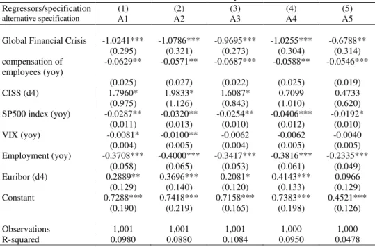
Table 4.a Robustness - Determinants of cyclical current account

Regressors/specification (1) (2) (3) (4) (5)

alternative specification A1 A2 A3 A4 A5

Global Financial Crisis -1.0241*** -1.0786*** -0.9695*** -1.0255*** -0.6788** (0.295) (0.321) (0.273) (0.304) (0.314) compensation of employees (yoy) -0.0629** -0.0571** -0.0687*** -0.0588** -0.0546*** (0.025) (0.027) (0.022) (0.025) (0.019) CISS (d4) 1.7960* 1.9833* 1.6087* 0.7099 0.4733 (0.975) (1.126) (0.843) (1.010) (0.620) SP500 index (yoy) -0.0287** -0.0320** -0.0254** -0.0406*** -0.0192* (0.011) (0.013) (0.010) (0.012) (0.010) VIX (yoy) -0.0081* -0.0100** -0.0062 -0.0062 -0.0040 (0.004) (0.005) (0.004) (0.005) (0.005) Employment (yoy) -0.3708*** -0.4000*** -0.3417*** -0.3816*** -0.2335*** (0.058) (0.065) (0.053) (0.061) (0.049) Euribor (d4) 0.2889** 0.3696*** 0.2081* 0.4143*** 0.0966 (0.129) (0.140) (0.120) (0.133) (0.129) Constant 0.7288*** 0.7418*** 0.7158*** 0.7383*** 0.4521*** (0.190) (0.219) (0.165) (0.198) (0.126) Observations 1,001 1,001 1,001 1,000 1,000 R-squared 0.0980 0.0880 0.1084 0.0950 0.0478

Note: Dependent variables are different versions of the cyclical component of the current account as detailed below (also refer to the main text for further explanations). Estimations of the yoy quarterly change of the cyclical cyclical component of the current account balance (percentage points of GDP). Hereroskedasticity and autocorrelation robust standard errors clustered at the country level in parenthesis. Estimation by Ordinary Least Squares and weighted least squares when TVC estimates are used (with weights given by the inverse of the standard deviation of the estimated TVC coefficient estimates). Constant term estimated but omitted for reasons of parsimony. *, **, *** denote statistical significance at the 10, 5 and 1 percent level, respectively.

A1: fixed elasticities and weights of 0.4 and 0.15 for the contemporaneous and lagged change in REER.

A2: fixed elasticities and slightly larger weights of 0.5 and 0.2 for the contemporaneous and lagged change in REER. A3: fixed elasticities and slightly smaller weights of 0.3 and 0.1 for the contemporaneous and lagged change in REER. A4: fixed elasticities and weights of 0.4, 0.2 and 0.1 for the contemporaneous, lagged and twice-lagged change in REER. A5: time-varying elasticities and weights of 0.4 and 0.15 for the contemporaneous and lagged change in REER, but the foreign economy corresponds to each country’s trading partners’ real GDP.

(22)

21

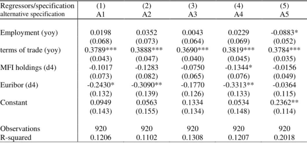
Table 4.b Robustness - Determinants of noncyclical current account

Regressors/specification (1) (2) (3) (4) (5)

alternative specification A1 A2 A3 A4 A5

Employment (yoy) 0.0198 0.0352 0.0043 0.0229 -0.0883* (0.068) (0.073) (0.064) (0.069) (0.052) terms of trade (yoy) 0.3789*** 0.3888*** 0.3690*** 0.3819*** 0.3784***

(0.043) (0.047) (0.040) (0.045) (0.035) MFI holdings (d4) -0.1017 -0.1283 -0.0750 -0.1344* -0.0156 (0.073) (0.082) (0.065) (0.076) (0.049) Euribor (d4) -0.2430* -0.3090** -0.1770 -0.3313** -0.0364 (0.132) (0.139) (0.126) (0.133) (0.115) Constant 0.0949 0.0563 0.1334 0.0534 0.2362** (0.143) (0.155) (0.134) (0.148) (0.114) Observations 920 920 920 920 920 R-squared 0.1206 0.1102 0.1308 0.1207 0.2018

Note: Dependent variables are different versions of the non-cyclical component of the current account as detailed below (also refer to the main text for further explanations). Estimations of the yoy quarterly change of the cyclical noncyclical component of the current account balance (percentage points of GDP). Hereroskedasticity and autocorrelation robust standard errors clustered at the country level in parenthesis. Estimation by Ordinary Least Squares and weighted least squares when TVC estimates are used (with weights given by the inverse of the standard deviation of the estimated TVC coefficient estimates). Constant term estimated but omitted for reasons of parsimony. *, **, *** denote statistical significance at the 10, 5 and 1 percent level, respectively.

A1: fixed elasticities and weights of 0.4 and 0.15 for contemporaneous and lagged change in REER.

A2: fixed elasticities and slightly larger weights of 0.5 and 0.2 for contemporaneous and lagged change in REER. A3: fixed elasticities and slightly smaller weights of 0.3 and 0.1 for contemporaneous and lagged change in REER. A4: fixed elasticities and weights of 0.4, 0.2 and 0.1 for contemporaneous, lagged and twice-lagged change in REER. A5: time-varying elasticities and weights of 0.4 and 0.15 for contemporaneous and lagged change in REER, but the foreign economy corresponds to each country’s trading partners’ real GDP.

(23)

22

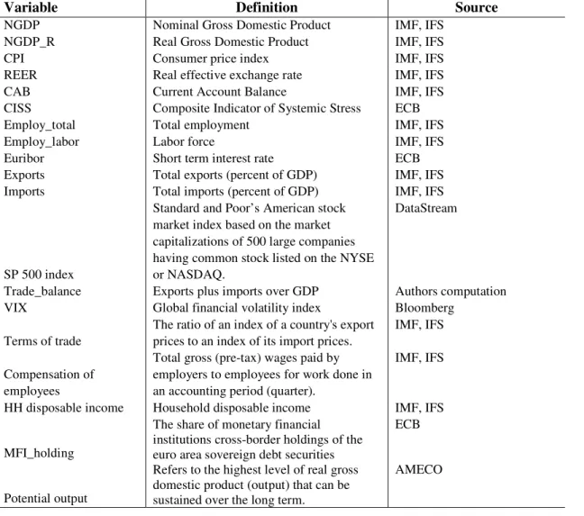
APPENDIX Table A.0 – Data sources

Variable Definition Source

NGDP Nominal Gross Domestic Product IMF, IFS NGDP_R Real Gross Domestic Product IMF, IFS CPI Consumer price index IMF, IFS REER Real effective exchange rate IMF, IFS CAB Current Account Balance IMF, IFS CISS Composite Indicator of Systemic Stress ECB Employ_total Total employment IMF, IFS Employ_labor Labor force IMF, IFS Euribor Short term interest rate ECB Exports Total exports (percent of GDP) IMF, IFS Imports Total imports (percent of GDP) IMF, IFS

SP 500 index

Standard and Poor’s American stock market index based on the market capitalizations of 500 large companies having common stock listed on the NYSE or NASDAQ.

DataStream

Trade_balance Exports plus imports over GDP Authors computation VIX Global financial volatility index Bloomberg

Terms of trade

The ratio of an index of a country's export prices to an index of its import prices.

IMF, IFS

Compensation of employees

Total gross (pre-tax) wages paid by employers to employees for work done in an accounting period (quarter).

IMF, IFS

HH disposable income Household disposable income IMF, IFS

MFI_holding

The share of monetary financial institutions cross-border holdings of the euro area sovereign debt securities

ECB

Potential output

Refers to the highest level of real gross domestic product (output) that can be sustained over the long term.

AMECO

Table A.1 Correlation Coefficients between cyclical and non-cyclical CA computed using TVC elasticities versus other alternative measures

cyclical TVC non-cyclical TVC cyclical A1 0.82 noncyclical A1 0.94 cyclical A2 0.77 noncyclical A2 0.93 cyclical A3 0.86 noncyclical A3 0.96 cyclical A4 0.81 noncyclical A4 0.94 cyclical A5 0.89 noncyclical A5 0.96 Source: authors’ computations.

(24)

23

Table A2. Determinants of cyclical current account, country by country

Specification/ (1) (2) (3) (4) (5) (6) (7) (8) (9)

Countries Austria Belgium France Germany Italy Luxembourg Netherland s Finland Greece Global Financial Crisis -0.0781 -3.1304 -0.2640 0.2891 -0.2692** 0.1976 0.0755 -0.0524 -0.2059 (0.161) (2.453) (0.167) (0.267) (0.123) (1.223) (0.250) (0.273) (0.310) compensation of employees (yoy) -0.4375*** (0.115) 6.0854*** (2.192) -0.2244** (0.093) -0.1912*** (0.067) -0.0857*** (0.025) -0.2276 (0.301) -0.0900 (0.123) -0.1586* (0.087) -0.0111 (0.025) CISS (d4) 1.1027** -3.6740 0.1024 0.0895 0.4535 4.3140 -0.4980 -0.2713 -0.1797 (0.518) (10.014) (0.340) (0.495) (0.408) (4.212) (1.030) (0.660) (0.918) SP500 index (yoy) 0.0171*** 0.0428 0.0031 0.0109* 0.0025 -0.1683*** 0.0126 -0.0217** -0.0227*** (0.006) (0.135) (0.004) (0.006) (0.005) (0.048) (0.014) (0.011) (0.008) VIX index (yoy) 0.0013 -0.0716 0.0015 0.0005 0.0027** -0.0512*** -0.0023 -0.0047 -0.0017 (0.002) (0.059) (0.001) (0.002) (0.001) (0.017) (0.003) (0.003) (0.003) Employment(yoy) -0.0678 -7.7062** 0.1031 -0.2153** 0.0178 0.8011 -0.0344 -0.0665 -0.2327*** (0.185) (3.569) (0.080) (0.096) (0.059) (0.831) (0.199) (0.184) (0.038) Euribor (d4) 0.4318*** -0.8670 0.0703 0.4512*** -0.0168 1.4874** 0.2632 0.0851 0.1094 (0.100) (1.865) (0.070) (0.088) (0.054) (0.657) (0.158) (0.213) (0.123) Observations 61 61 61 61 44 60 48 61 61 R-squared 0.4293 0.3585 0.2241 0.5042 0.4294 0.3815 0.4198 0.3831 0.5978

Note: Dependent variable is the cyclical component of the current account for each country identified in the second row. Estimations of the yoy quarterly change of the cyclical noncyclical component of the current account balance (percentage points of GDP). Hereroskedasticity and autocorrelation robust standard errors in parenthesis. Estimation by Ordinary Least Squares. Constant term estimated but omitted for reasons of parsimony. *, **, *** denote statistical significance at the 10, 5 and 1 percent level, respectively.

Table A2. Determinants of cyclical current account, country by country (cont.)

Specification/ (1) (2) (3) (4) (5) (6) (7) (8) Countries Ireland Portugal Spain Slovakia Estonia Latvia Lithuania Slovenia Global Financial Crisis -1.3195*** -0.6619*** -1.0128*** 0.2185 -1.1964 -1.3136*** -0.3813 -1.4678 (0.367) (0.179) (0.204) (0.790) (1.348) (0.413) (1.205) (0.932) compensation of employees (yoy) -0.0485 -0.1350*** -0.0336 -0.3916*** -0.1879* -0.0659*** -0.1885** -0.1886* (0.056) (0.028) (0.030) (0.137) (0.112) (0.022) (0.085) (0.095) CISS (d4) -1.1142 -2.0831*** -0.3347 -1.5126 8.5092*** 2.3582 5.7921* 1.2896 (0.913) (0.717) (0.373) (2.054) (2.961) (1.708) (3.227) (1.551) SP500 index (yoy) 0.0070 -0.0301*** 0.0043 -0.0216 0.0408 0.0313* 0.0091 -0.0384** (0.011) (0.007) (0.004) (0.029) (0.025) (0.017) (0.035) (0.019) VIX index (yoy) -0.0029 -0.0025 0.0003 0.0009 0.0262** 0.0189** 0.0159 0.0021 (0.004) (0.002) (0.002) (0.008) (0.011) (0.007) (0.013) (0.006) Employment(yoy) -0.1546 -0.0533 -0.1606*** 0.2303* -0.3111*** -0.1086* -0.4151** -0.4528*** (0.098) (0.060) (0.023) (0.125) (0.113) (0.056) (0.168) (0.159) Euribor (d4) 0.8674*** 0.3860*** 0.1261* -0.8497* -0.7049 -0.0601 -0.8846** -0.7404*** (0.124) (0.076) (0.065) (0.483) (0.531) (0.221) (0.377) (0.252) Constant 0.9555** 0.8746*** 0.9070*** 1.6311 1.7194 0.7871* 0.5653 1.4999* (0.378) (0.171) (0.170) (1.199) (1.628) (0.397) (1.058) (0.811) Observations 61 62 60 56 61 60 61 61 R-squared 0.5475 0.5638 0.6554 0.5387 0.6600 0.5300 0.6379 0.6710

Note: Dependent variable is the cyclical component of the current account for each country identified in the second row. Estimations of the yoy quarterly change of the cyclical noncyclical component of the current account balance (percentage points of GDP). Hereroskedasticity and autocorrelation robust standard errors in parenthesis. Estimation by Ordinary Least Squares. Constant term estimated but omitted for reasons of parsimony. *, **, *** denote statistical significance at the 10, 5 and 1 percent level, respectively.

(25)

24

Table A3. Determinants of non-cyclical current account, country by country

Specification/ (1) (2) (3) (4) (5) (6) (7) (8) (9) Countries Austria Belgium France Germany Italy Luxembourg Netherlands Finland Greece Employment(yoy) 0.5690 -1.7913* 0.0629 0.1911 -0.3166* -3.2290 0.1210

-0.0271

-0.3504** (0.432) (1.021) (0.091) (0.425) (0.172) (1.969) (0.299) (0.324) (0.137) terms of Trade (yoy) -0.0792 0.4479 -0.0532 0.1753* 0.1516** -0.8319 -0.8861*** 0.0448 0.2053 (0.197) (0.410) (0.059) (0.103) (0.060) (0.833) (0.288) (0.114) (0.171) MFI holdings (d4) 0.0740 -0.2382 0.0138 -0.0420 0.0676 -0.6499 0.2217 0.0546 0.1448 (0.104) (0.195) (0.038) (0.128) (0.070) (0.545) (0.140) (0.168) (0.199) Euribor (d4) -0.2776 -0.0536 -0.2250 -0.1623 0.1037 -0.0380 -0.6872*** 0.3738 -0.6602*** (0.341) (0.688) (0.135) (0.207) (0.260) (0.723) (0.243) (0.363) (0.227) Constant -0.1351 0.9914 -0.1746 0.7407*** 0.3086*** 5.2456 0.4679 -0.3927 -0.4700 (0.465) (0.963) (0.119) (0.274) (0.114) (3.917) (0.339) (0.297) (0.369) Observations 56 56 56 56 40 56 44 56 56 R-squared 0.0312 0.2026 0.1004 0.1162 0.2505 0.0714 0.3059 0.0260 0.2658

Note: Dependent variable is the non-cyclical component of the current account for each country identified in the second row. Estimations of the yoy quarterly change of the noncyclical noncyclical component of the current account balance (percentage points of GDP). Hereroskedasticity and autocorrelation robust standard errors in parenthesis. Estimation by Ordinary Least Squares. Constant term estimated but omitted for reasons of parsimony. *, **, *** denote statistical significance at the 10, 5 and 1 percent level, respectively.

Table A3. Determinants of non-cyclical current account, country by country (cont.)

Specification/ (1) (2) (3) (4) (5) (6) (7) (8) Countries Ireland Portugal Spain Slovakia Estonia Latvia Lithuania Slovenia Employment(yoy) -0.2278* -0.6794*** -0.3782*** 0.6734*** 0.2690** 0.2686* 0.5022*** -0.1088

(0.124) (0.120) (0.062) (0.178) (0.129) (0.158) (0.133) (0.108) terms of Trade (yoy) -0.0549 0.5759*** 0.3012*** 0.8138*** 0.4323*** 0.5579*** 0.3786*** 0.3540***

(0.129) (0.117) (0.085) (0.087) (0.087) (0.051) (0.060) (0.059) MFI holdings (d4) 0.0737 -0.1468* 0.0954 -0.2989 0.1063 0.0932 0.3103* 0.3651*** (0.166) (0.083) (0.084) (0.191) (0.210) (0.216) (0.167) (0.110) Euribor (d4) -0.6101 0.3875 -0.0615 -1.2265* 0.3348 -1.7966*** -0.1615 1.1427*** (0.384) (0.274) (0.274) (0.656) (0.462) (0.568) (0.448) (0.291) Constant 0.3968 -0.0455 0.4850** -0.4583 0.4041 -0.7093* 1.3777*** 0.9003*** (0.374) (0.235) (0.234) (0.495) (0.454) (0.400) (0.386) (0.245) Observations 56 56 56 52 56 56 56 56 R-squared 0.2673 0.5838 0.7424 0.6181 0.4184 0.7944 0.5153 0.4602

Note: Dependent variable is the non-cyclical component of the current account for each country identified in the second row. Estimations of the yoy quarterly change of the noncyclical noncyclical component of the current account balance (percentage points of GDP). Hereroskedasticity and autocorrelation robust standard errors in parenthesis. Estimation by Ordinary Least Squares. Constant term estimated but omitted for reasons of parsimony. *, **, *** denote statistical significance at the 10, 5 and 1 percent level, respectively.

(26)

25

Figure A1.a Time-Varying Coefficient Model Estimates of Elasticities, Country-by-country time profile 1999Q1-2015Q4 1 .8 61 .8 8 1 .9 1 .9 2 2 .2 5 2 .3 2 .3 5 .7 .8 .9 1 .8 2 2 8 2 .8 2 2 8 4 .8 2 2 8 6 .8 2 2 8 8 2 .2 2 0 2 2 .2 2 0 3 2 .2 2 0 4 2 .2 2 0 5 2 .0 42 .0 62. 0 82 .1 2 .1 2 2 .5 2 .5 12. 5 22 .5 32 .5 4 .8 .8 5 .9 .9 5 1 .8 5 .9 .9 5 1 1 .9 8 2 2 .0 22 .0 4 .9 2 1 2 7 .9 2 1 2 7 5 .9 2 1 2 8 .9 2 1 2 8 5 1 .4 3 2 6 1 .4 3 2 6 2 1 .4 3 2 6 4 1 .4 3 2 6 6 1 .4 3 2 6 8 1 .5 4 7 91. 5 4 7 9 51 .5 4 8 .7 3 6 2.7 3 6 25.7 3 6 3.7 3 6 3 5 1 .7 61 .7 81 .8 1 .8 21 .8 4 1 .4 5 1 .5 1 .5 5 1 .6 .4 4 8 5 5 2 .4 4 8 5 5 1 .4 51 .5 1 .5 51 .6 1 .0 61 .0 81 .1 1 .1 21 .1 4 2000q12005q12010q12015q1 2000q12005q12010q12015q1 2000q12005q12010q12015q1 2000q12005q12010q12015q1 2000q12005q12010q12015q1

Austria Belgium Cyprus Estonia Finland

France Germany Greece Ireland Italy

Latvia Lithuania Luxembourg Malta Netherlands

Portugal Slovak Republic Slovenia Spain

th e ta _ x qdate

TVC-income elasticity of exports

-1 .2-1 .1 5-1 .1-1 .0 5-1 -. 5 5-.5 -. 4 5-.4 -. 3 5 -. 8 -. 7 5 -. 7 -. 6 5 .6 .7 .8 .9 -. 7 -. 6 5 -. 6 -. 5 5 -. 8 -. 7 5 -. 7 -. 6 5 -1 .1-1 .0 5-1 -. 9 5-.9 -. 5 -. 4 -. 3 -1 .3 -1 .2 -1 .1 -1 -1 .0 5 -1 -. 9 5 -. 9 -. 4 -. 2 0 -. 8 -. 6 -. 4 -. 2 -. 8 -. 7 -. 6 -. 5 -. 5 -. 4 -. 3 -. 2 -1 .2-1 .1 5-1 .1-1 .0 5-1 -. 5-.4 5-.4 -. 3 5-.3 .2 .3 .4 .5 .6 -. 7 -. 6 -. 5 -. 4 -. 3 -. 0 5 0 .0 5 .1 .1 5 2000q12005q12010q12015q1 2000q12005q12010q12015q1 2000q12005q12010q12015q1 2000q12005q12010q12015q1 2000q12005q12010q12015q1

e

ta

_

x

qdate

(27)

26

Note: theta_x stands for the income elasticity of exports; eta_x stands for the elasticity of exports with respect to the real effective exchange rate; theta_m stands for the income elasticity of imports; eta_m stands for the elasticity of imports with respect to the real effective exchange rate.

Source: authors’ computations (see equation (1)).

1 .7 1 .7 21 .7 41 .7 61 .7 8 2 .3 5 2 .4 2 .4 5 2 .5 .9 .9 5 1 1 .0 51 .1 1 .1 0 5 5 2 1 .1 0 5 5 4 1 .1 0 5 5 6 1 .1 0 5 5 8 1 .8 4 5 1 1 .8 4 5 1 2 1 .8 4 5 1 4 1 .8 4 5 1 6 1 .8 4 5 1 8 2 .4 42 .4 62. 4 82 .52 .5 2 1 .7 81 .7 91 .8 1 .8 11 .8 2 1 .1 11 .1 21 .1 31 .1 41 .1 5 .3 .4 .5 .6 2 .1 22 .1 42 .1 62 .1 82 .2 .6 9 .7 .7 1. 7 2 .7 3 1 .5 9 4 8 8 1 .5 9 4 9 1 .5 9 4 9 2 1 .5 9 4 9 4 1 .1 51 .2 1 .2 51 .3 1 .3 5 .6 9 .7 .7 1. 7 2 .7 3 1 .7 1 .7 21 .7 41 .7 61 .7 8 1 .5 1 .5 5 1 .6 1 .6 5 1 .3 9 6 421. 3 9 6 4 31. 3 9 6 4 3 .7 5 7 1 4 2 .7 5 7 1 4 1 .4 5 1 .5 1 .5 5 1 .6 2000q12005q12010q12015q1 2000q12005q12010q12015q1 2000q12005q12010q12015q1 2000q12005q12010q12015q1 2000q12005q12010q12015q1

th e ta _ m qdate

TVC-income elasticity of imports

-1 .0 5 -1 -. 9 5 -. 9 -. 6 5-.6 -. 5 5-.5 -. 4 5 -. 8 -. 7 -. 6 .2 .3 .4 .5 -. 9 -. 8 -. 7 -. 9 5 -. 9 -. 8 5 -. 8 -1 .2 5-1 .2 -1 .1 5-1 .1 -. 9 -. 8 -. 7 -. 6 -1 -. 9 -. 8 -. 7 -1 .4-1 .3 5-1 .3-1 .2 5-1 .2 -. 8 -. 7 -. 6 -. 5 -. 4 -1 .5 -1 -1 -. 9 -. 8 -. 7 -. 2 -. 1 0 .1 -1 .2-1 .1 5-1 .1-1 .0 5-1 -. 9 5 -. 9 -. 8 5 -. 8 -. 3 -. 2 -. 1 0 .1 -. 7 -. 6 -. 5 -. 4 -. 0 5 0 .0 5 .1 .1 5 2000q12005q12010q12015q1 2000q12005q12010q12015q1 2000q12005q12010q12015q1 2000q12005q12010q12015q1 2000q12005q12010q12015q1

e

ta

_

m

qdate

(28)

27

Figure A2.a Non-cyclical current account (% GDP), Country-by-country time profile 1999Q1-2015Q4

Figure A2.b Cyclical current account (% GDP), Country-by-country time profile 1999Q1-2015Q4

-2 0 2 4 6 0 2 0 4 0 6 0 -2 0-1 5-1 0 -5 0 -2 0 -1 0 0 1 0 -5 0 5 1 0 -2 0 2 4 -5 0 5 1 0 -1 5 -1 0 -5 0 -1 0 0 1 0 2 0 -4 -2 0 2 -2 0 -1 0 0 1 0 -1 0 0 1 0 -1 0 0 1 0 2 0 -2 0 -1 0 0 1 0 0 5 1 0 1 5 -1 5 -1 0 -5 0 -1 5-1 0 -5 0 5 -5 0 5 1 0 -1 0 -5 0 2000q12005q12010q12015q1 2000q12005q12010q12015q1 2000q12005q12010q12015q1 2000q12005q12010q12015q1 2000q12005q12010q12015q1

n o n c y c lic a l_ c a _ tv c qdate -3 -2 -1 0 1 -6 0 -4 0 -2 0 0 -4 -2 0 2 4 -1 0 -5 0 5 -2 -1 0 1 -1 .5 -1 -. 5 0 .5 -4 -2 0 2 -2 0 2 4 -4 -2 0 2 -. 5 0 .5 1 -5 0 5 -1 0 -5 0 5 1 0 -1 0 -5 0 5 1 0 -4 -2 0 2 -2 0 2 4 -2 0 2 -1 0 -5 0 5 1 0 -1 0 -5 0 5 -2 0 2 4 2000q12005q12010q12015q1 2000q12005q12010q12015q1 2000q12005q12010q12015q1 2000q12005q12010q12015q1 2000q12005q12010q12015q1

c y c lic a l_ c a _ tv c qdate