EQUITY RESEARCH: AN EVALUATION OF EDP’S TENDER
OFFER OVER EDP RENOVÁVEIS
Gonçalo Manuel Martinho Heitor
Project submitted as partial requirement for the conferral of Master in Finance
Supervisor:
Prof. António Gomes Mota, Full Professor, ISCTE Business School, Department of Finance
To my sister Mariana, who is now starting this amazing journey.
“Education is the most powerful weapon which you can use to change the world.” Nelson Mandela
i Resumo
A crescente competitividade no custo das tecnologias (principalmente eólica e solar), o aumento no consumo de eletricidade e as rígidas políticas governativas rumo à descarbonização da economia são alguns dos principais desafios que têm, cada vez mais, transformado o sector das energias renováveis.
Uma das empresas que se encontra em posição favorável nesta revolução em curso é a EDP Renováveis, dedicando-se à produção de energia exclusivamente através de fontes renováveis, particularmente eólica onshore.
Assim, para incrementar a exposição ao crescimento das renováveis, o maior acionista (EDP - Energias de Portugal) lançou, a 27 de março de 2017, uma Oferta Pública de Aquisição (OPA) sobre os 22.47% de capital que não controlava na subsidiária, a um preço de 6.75€ por ação. Esta dissertação apresenta uma análise, a 31 de março de 2017, e consequente definição de um preço-alvo para a ação no final do ano de 2017. Foi também possível analisar se o valor oferecido pela EDP era justo e se os acionistas minoritários estariam, ou não, dispostos a aceitá-lo.
Um modelo DCF, alicerçado na soma das partes, assinala um preço-alvo de €7.83, ou seja, uma apreciação de 13%, o que indica que o valor oferecido pela EDP não reconhece verdadeiramente o valor intrínseco e o crescimento potencial da empresa.
Concluindo, o desempenho histórico positivo aliado a uma abordagem de baixo risco na exposição a mercado atraentes, como os Estados Unidos, são essenciais para reforçar uma recomendação de Compra, considerando que o mercado não reflete o correto valor da EDP Renováveis.
Palavras-Chave: Value of Firm; Equity Research; Valuation; Renewable Energy
Código de Classificação JEL: G32 – Financing Policy; Financial Risk and Risk Management;
Capital and Ownership Structure; Value of Firms; Goodwill
ii Abstract
The increasing cost competitiveness of renewable technologies (mainly wind power and solar PV), the continuous increase in global electricity demand and strict government policies towards the decarbonisation of the economy are some of the main challenges and growth opportunities that have been increasingly transforming the renewable energy industry.
One of the companies in the front row of this ongoing revolution is EDP Renováveis, focused exclusively on the generation of energy from renewable sources, primarily wind onshore. Hence, to benefit even more from the attractive growth of EDPR, its major shareholder (EDP - Energias de Portugal) launched on 27 March 2017 a tender offer to buy-back the 22.47% of share capital it did not hold in the subsidiary, at a price of €6.75 per share.
This dissertation presents, as of 31 March 2017, a comprehensive analysis and consequent estimation of the fair value of EDP Renováveis, by targeting a price for the year-end 2017. Consequently, it allowed for the fair evaluation of EDP’s offer and to answer whether minority shareholders should be willing to accept it or not.
Accordingly, a sum-of-the-parts DCF valuation derives a target price of €7.83 per share, i.e., a 13% upside, which clearly indicates that the price offered by EDP did not truthfully reflected the fundamental value of the company and its potential growth.
Overall, the positive historical performance and low-risk approach to attractive markets, such as the United States, are fundamental to support a buy recommendation, considering the market might be undervaluing the stock.
Keywords: Value of Firm; Equity Research; Valuation; Renewable Energy
JEL Classification Code: G32 – Financing Policy; Financial Risk and Risk Management;
Capital and Ownership Structure; Value of Firms; Goodwill
iii Table of Contents 1. Introduction ... 1 2. Review of literature ... 3 2.1. Fundamentals of Valuation ... 3 2.2. Valuation Methods ... 3 2.2.1. Introduction ... 3
2.2.2. Discounted Cash Flow Models ... 4
2.2.2.1. FCFF - Free Cash Flow to the Firm ... 4
2.2.2.1.1. Required return on Equity ... 5
2.2.2.1.1.1. Risk-Free Rate ... 5
2.2.2.1.1.2. Beta ... 6
2.2.2.1.1.3. Market Risk Premium ... 7
2.2.2.1.2. Cost of Debt ... 8
2.2.2.1.3. Target Capital Structure... 8
2.2.2.1.4. Taxes ... 9
2.2.2.1.5. Terminal Value ... 9
2.2.2.2. FCFE – Free Cash Flow to Equity ... 11
2.2.2.3. APV - Adjusted Present Value ... 12
2.2.2.3.1. Interest tax shields ... 13
2.2.2.3.2. Expected Bankruptcy Costs ... 14
2.2.3. DDM - Dividend Discount Model ... 14
2.2.4. Relative Valuation ... 15
2.2.5. EVA -Economic Value Added Model ... 17
2.3. Valuation of Utilities and Renewable Energy ... 18
2.4. Cross-Border Valuation ... 18
3. Company and Market Overview ... 21
3.1. Renewable Energy Industry ... 21
3.1.1. Introduction ... 21
3.1.2. Macroeconomic Outlook ... 22
3.1.2.1. Wind Energy ... 22
3.1.2.2. Solar Energy ... 23
3.2. EDP Renováveis S.A. ... 25
3.2.1. General Description ... 25
3.2.2. Shareholder Structure ... 25
3.2.3. Company Performance ... 26
iv
3.2.5. Markets and Regulatory Framework ... 28
3.2.5.1. Europe ... 28 3.2.5.2. North America ... 30 3.2.5.3. Brazil ... 31 3.2.6. Strategic Outlook ... 31 4. Valuation ... 35 4.1. Introduction ... 35
4.2. Assumptions and Forecasts ... 36
4.2.1. Balance Sheet and Income Statement estimation ... 36
4.2.1.1. Revenues ... 36
4.2.1.2. Operating Costs ... 39
4.2.1.3. Depreciation and Amortization ... 40
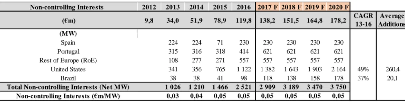
4.2.1.4. Non-controlling interests ... 40
4.2.2. Capital Expenditures ... 41
4.2.3. Working Capital ... 42
4.2.4. Discount rate – WACC ... 42
4.2.4.1. Capital Structure ... 42
4.2.4.2. Cost of Equity ... 43
4.2.4.2.1. Risk-free rate ... 43
4.2.4.2.2. Beta Estimation ... 44
4.2.4.2.3. Market Risk Premium ... 45
4.2.4.3. Tax Rate ... 45
4.2.4.4. Cost of Debt ... 46
4.2.4.5. Summary ... 46
4.3. Discounted Free Cash Flow Valuation ... 47
4.3.1. Continuing Value ... 47
4.3.2. EDP Renováveis’ fair value ... 48
4.3.3. Sensitivity and Scenario Analysis ... 50
4.3.4. Other DCF approaches ... 51
4.3.4.1. Discounted FCFE ... 51
4.3.4.2. Adjusted Present Value ... 52
4.4. Relative Valuation ... 53
4.4.1. Enterprise Value to EBITDA ... 53
4.4.2. Price-Earnings Ratio ... 54
4.4.3. Enterprise Value to Megawatt ... 54
5. Comparative Analysis ... 57
v
7. Conclusion ... 61
8. Bibliography ... 63
9. Appendices ... 67
Appendix A – Paris Climate Change Agreement ... 67
Appendix B – Global Energy Outlook ... 68
Appendix C - Global Wind Outlook... 69
Appendix D - Global Solar Outlook ... 72
Appendix E – Geographical Distribution of EDPR... 73
Appendix F – Operational data detail for the term 2013-2016 ... 74
Appendix G – Regulatory framework on EDPR’s geographies ... 75
Appendix H – PTC and ITC framework ... 77
Appendix I – EDPR’s load factor and availability ... 77
Appendix J – Self-Funding Business Model description ... 78
Appendix K – Installed capacity additions for the term 2016-2020 -EDPR Plans ... 78
Appendix L – Individual Income Statements ... 79
Appendix M – Consolidated Income Statement ... 81
Appendix N– Consolidated Balance Sheet ... 82
Appendix O – Revenues Estimation ... 84
Appendix P – Estimated Installed Capacity (MW) Additions ... 84
Appendix Q – Consolidated Working Capital ... 85
Appendix R – Debt Map ... 85
Appendix S – Synthetic rating estimation ... 86
Appendix T– FCFF valuation ... 86
Appendix U– Sensitivity and Scenario Analysis ... 88
Appendix V– FCFE valuation ... 89
Appendix W– APV Valuation ... 91
Appendix X– Multiples Valuation ... 93
vi
Index of Figures
Figure 1: Global Levelized Cost of Energy ($/MWh) ... 21
Figure 2: World electricity demand and related CO2 emissions ... 22
Figure 3: Market Performance since the IPO (Initial Public Offer) ... 27
Figure 4: EBITDA per Business Unit (m€) ... 36
Figure 5: Electricity Sales (m€/MW) ... 37
Figure 6: 2016-2020 estimated capacity additions (MW) ... 38
Figure 7: Geographical Breakdown of installed capacity (%) ... 39
Figure 8: Operating Costs per MW (m€/MW) ... 39
Figure 9: D&A over previous year net PP&E and Intangibles (%) ... 40
Figure 10: Capital Expenditures (€m) ... 41
Index of Tables Table 1: Most commonly used multiples ... 15
Table 2: EDPR’s Operational Summary 2013-2016 ... 26
Table 3: EDPR’s Financial Summary 2013-2016 ... 26
Table 4: Non-Controlling interests estimates ... 41
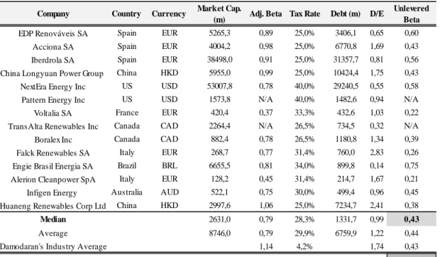
Table 5: Bottom-up Beta ... 44
Table 6: Country Risk Premium... 45
Table 7: Corporate marginal tax rates ... 45
Table 8: Synthetic rate estimation ... 46
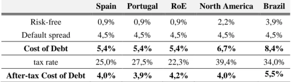
Table 9: Cost of Debt ... 46
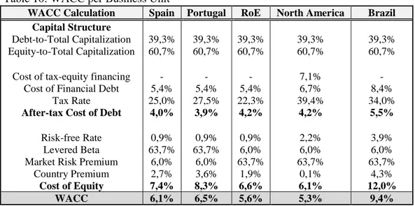
Table 10: WACC per Business Unit ... 47
Table 11: Perpetuity growth rates ... 48
Table 12: Sum-of-the-parts FCFF Valuation ... 48
Table 13: Target Price (€) ... 50
Table 14: Target Price variation (%) ... 50
Table 15: FCFE Valuation ... 51
Table 16: Adjusted Present Value Valuation ... 52
Table 17: EV/EBITDA multiples ... 53
Table 18: Price-Earnings multiples ... 54
Table 19: Fair Value at asset rotation multiples ... 55
Table 20: Comparative Analysis of valuation estimates ... 57
Table 21: Target price consensus ... 59
vii List of Abbreviations
APV – Adjusted Present Value
CAPM – Capital Asset Pricing Model CAPEX – Capital Expenditures COP - Conference of Parties DCF -Discounted Cash Flow DPS -Dividends per Share
EBIT – Earnings Before Interest and Taxes EDPR – EDP Renováveis
EQV -Equity Value EV -Enterprise Value
EV/EBITDA – Enterprise Value to EBITDA EV/EG – Enterprise Value to EBITDA growth EV/FCF – Enterprise Value to Free Cash Flow EV/Sales – Enterprise Value to Sales
EVA – Economic Value Added FCFE – Free Cash flow to Equity FCFF – Free Cash Flow to the Firm FiT – Feed-in-Tariff
GDP - Gross Domestic Product GW – Gigawatt
GWEC – Global Wind Energy Council IC – Invested Capital
IEA – International Energy Agency
IRENA – International Renewable Energy Agency LCOE – Levelized Cost of Energy
NOPLAT – Net Operating Profit Less Adjusted Taxes OPEX – Operating Expenses
P/BV – Price to Book Value P/CE – Price to Cash Earnings PEG – Price Earnings Growth PER – Price Earnings Ratio PPA – Power Purchase Agreement P/S – Price to Sales
PV – Photovoltaic
ROIC – Return on Invested Capital SOTP –Sum-of-the-parts
WC – Working Capital
1 1. Introduction
Valuation assumes an essential role in the life of a company since it not only allows the fair value estimation of a business for potential transactions, but is also a source of information about the main risks and sources of growth, enhancing the decision-making process regarding the company’s business strategy.
Driven by the opportunity to put in practice all the concepts related to equity valuation learned during the academic curriculum, this dissertation has the main objective of delivering the right framework and proceed to the fair value estimation of EDP Renováveis S.A. (hereinafter referred to as “EDP Renováveis” or “EDPR”).
In this matter, this is also the opportunity to study in detail a company that has a leading position in terms of innovation and sustainability, within an industry facing constant challenges and growth opportunities.
In fact, the increase in cost competitiveness of renewable technology and the political pressure for the decarbonisation of the economy, reinforced by the recent COP 21 agreement reached in Paris, has put EDPR in a favourable position to this transition towards a more efficient and clean energy production worldwide.
Created as the renewable subsidiary of EDP S.A. (a vertically-integrated utility company), EDP Renováveis is currently headquartered in Madrid and listed in the Euronext Lisbon since 2008. The company is a global leader in the renewable energy sector, with an installed capacity of 10.4 GW (gigawatts) as of 31 March 2017, being the fourth biggest wind power producer in the world.
As such, in order to incorporate all these growth prospects, EDP (owner of 77.53% of the company) launched, on 27 March 2017, a tender offer to buy the remaining outstanding shares at €6.75, expecting to attain more than 90% of total shares (and voting rights) and withdraw EDPR from the stock exchange.
So, this project aims to answer the major research question “What is the fair value of EDP Renováveis’ share?” and, therefore, provide a recommendation to potential investors, based on the target price for the year-end 2017. Correspondingly, this study also intends to examine what should be the expected reaction of the remaining shareholders to EDP’s market proposal of €6.75 per share.
All things considered, the first section of this project focus on the literature review, containing a detailed description of the main valuation methodologies and all their essential inputs, as well
2
as a brief comparison among them. A note about the assessment of renewable energy utilities and multinational companies is also added to this conceptual review.
The next section includes a comprehensive description of EDPR’s business, its historical performance, shareholder structure, regulatory framework and main strategic drivers. This also includes an overview of the industry, describing the competitive environment and the main threats and opportunities in the renewable energy sector.
Afterwards, the main segment is centred in the valuation of EDP Renováveis. Taking into account all the available information, performance forecasts and assumptions, different valuation models are performed in order to define a target price for the company’s stock by the end of 2017.
This research report is primarily based on the DCF (Discounted Cash Flow) methodology, through the FCFF (Free Cash Flow to the Firm) discounted at the WACC (Weighted Average Cost of Capital), since it is the most widespread practice to value renewable energy companies among analysts.
Additionally, a sensitivity analysis will also be necessary to define what supports the final value estimated, providing meaningful insights to both investors and EDPR’s decision makers. Nonetheless, other DCF methodologies are also presented, namely the Adjusted Present Value (APV) and the FCFE (Free Cash Flow to Equity), as a confirmation tool for the previous results. In the same way, the Equity value of EDPR was estimated based on forward multiples for 2017. Moreover, a comparative analysis is presented in Chapter 5, in which the estimates and results of this research are compared with the targets of EDPR’s business plan and the reports of analysts from BPI - Banco Português de Investimento (27 March 2017) and Santander (27 March 2017).
Chapter 6 will be the end-point of this project, in which the current (31 March 2017) market price is compared with the target price for 2017, resulting in a final recommendation based on the total expected return. Lastly, also taking into consideration the expectation of returns within the next months, the tender offer of EDP to current equity holders is analysed, as of 31 March 2017.
3 2. Review of literature
2.1. Fundamentals of Valuation
Regardless of the company being valued, the process should not only focus on the financial/qualitative aspects of the firm, but also on all non-financial resources and strategic outlook presented in its business plan. Thus, before assessing the value of any company, it is important to fully understand its market situation, business model and all the macroeconomic and regulatory framework related to its operations (Damodaran, 2012).
Moreover, equity valuation can play distinct roles, representing a valuable tool for investors while taking portfolio management decisions. Valuation reports not only allow the analysis and comparison of various target companies but are also used to compare its intrinsic value with the stock price on the market and make an informed investment decision: buy, sell or hold. Similarly, equity valuation is widely used in corporate transactions such as mergers and acquisitions, representing a tool to back up negotiations between the parties; it is also a major factor in the process leading to stock market listing (IPO) or delisting (takeovers).
Koller, Goedhart and Wessels (2005) state that “managers who focus on shareholder value create healthier companies,” therefore they should put their efforts into long-term value rather than quarterly earnings. In this perspective, valuation is also important for corporate strategy, allowing managers to continuously rethink and measure the impact of their decisions on the creation or destruction of company’s long-term sustainable value.
2.2. Valuation Methods 2.2.1. Introduction
Even though there is an extensive amount of literature and several different categorisations to the valuation process, Damodaran (2012) establishes three general valuation methodologies: Discounted cash-flow valuation, relative (multiples) valuation and contingent claim valuation. The latter, which uses option pricing theory, has limited applications due to difficulties in estimating the inputs and control the risk sources, which results in its lack of utilisation for valuation purposes (Koller, Goedhart and Wessels, 2005).
Therefore, in this section, the focus will be in the detailed analysis of the other two methodologies.
4
2.2.2. Discounted Cash Flow Models
The discounted cash Flow (DCF) models are the most commonly used by analysts and equity researchers due to its dynamic and forward-looking perspective, not being dependent on past performance. These models claim that the value of a company corresponds to the present value of the expected cash-flows that will be generated in the future, discounted at the most appropriate discount rate (Fernández, 2005).
Two different concepts of cash flows can be used: The Free Cash Flow to the Firm (FCFF) and the Free Cash Flow to Equity (FCFE).
2.2.2.1. FCFF - Free Cash Flow to the Firm
The Free Cash Flow to the Firm corresponds to the after-tax cash-flow generated by operations that is available to investors, after deducting all the expenses, including working capital and net capital expenditures, needed to support company’s operations.
Therefore, starting from deducting taxes directly from the operating income (Earnings Before Interest and Taxes), the depreciation for the period should be added, since it is an accounting (non-cash) item. Moreover, the new investments in fixed assets and the working capital requirements should be subtracted to get the final FCFF, as follows:
FCFF = EBIT (1 - t) + Depreciations - Capital Expenditures (CAPEX)
± Changes in Working Capital (∆WC)
(1)
Since the Free Cash Flows to the Firm are the sum of the cash-flows related to all investors (including bondholders and stockholders), their discount rate should take into consideration the risk of all claim holders in the company. Therefore, as Fernández (2011) state, the discount rate should be a weighted average of two measures: the cost of debt (rD) and the required return on equity (rE).
Thus, this Weighted Average Cost of Capital (WACC) will have the following formulation:
WACC = E E + D× rE + D E + D × rD × (1 - t) (2)
D and E are, respectively, the market values of Debt (interest-bearing) and Equity of the firm. Moreover, the cost of debt (rD) is reduced by the marginal tax rate (t) to account for the interest tax shields generated by the interest payments on the outstanding debt.
5 To get the most appropriate rate of return, three essential inputs should be accounted carefully: required return on equity, cost of debt and the targeted capital structure for the company.
2.2.2.1.1. Required return on Equity
Some risk and return models attempt to find the correct expected return on the investment, such as the three-factor model introduced by Fama and French (1993) or the Arbitrage Pricing Theory (APT). Nevertheless, the most commonly used method is the Capital Asset Pricing Model - CAPM, firstly presented by William Sharpe (1964).
The CAPM is a single-factor model that assumes the expected return on equity equals the risk-free rate plus the beta of the security multiplied by the market risk premium (expected return on the market over risk-free rate), as presented in equation 3. (Elbannan, 2014).
rE = rf + βL × [ E(rM) - rf ] (3)
r f = risk free rate
𝛽𝐿 = Equity beta of the company
E (rM) = expected return on the market index
2.2.2.1.1.1. Risk-Free Rate
According to Damodaran (2008), the risk-free rate is the return on investments that, theoretically, satisfy two essential conditions. First, no default risk, which means only a few government securities might have the possibility to be completely risk-free. Second, no reinvestment risk, meaning it should ideally have the same duration as the cash-flow being discounted.
Due to difficulties in estimating the rate bearing in mind the exact previous conditions, Copeland, Koller and Murrin (2008) outline three different alternatives to use:(1) government treasury (short-term) bills, (2) ten-year treasury bond rate and (3) thirty-year treasury bond rate. The authors state that, for simplicity, it is recommended the yield-to-maturity of the long-term government bonds that better match the features of the stream of cash-flows, usually the 10-year risk-free government bond1.
Correspondingly, providing its consistency with the currency in which the cash-flows are estimated, this option is the one that better approximates the duration of the cash-flows and is less sensitive to fluctuations in inflation and liquidity.
6
The main issues in assessing risk-free rates arise when a country is not default-free or has only long-term bonds outstanding in a currency that is not the domestic one, which takes importance when valuing companies in emerging markets.
Damodaran (2008) suggests that this can be achieved using the rate of an entirely risk-free country, such as the United States, scaling it up by the differential inflation between the US and the currency in question, as follows:
risk-free Currency= (1 + risk-free US) ×
(1 + expected inflation foreign currency) (1 + expected inflation US) - 1
(4)
2.2.2.1.1.2. Beta
The beta (β) is a measure of systematic risk and reflects how a stock behaves to changes in the market. It is dependent on three main variables: the type of business of the company, its degree of operating level and the financial leverage.
It is commonly estimated by regressing the returns of the stock against the market returns, using the market model (Koller et al., 2005), where the slope corresponds to the beta, as follows:
Koller et al. (2005) also argue that the regression should be based on monthly returns (with at least five years of data) and regressed against a value-weighted and diversified market index. However, Damodaran (1999a) provides evidence that this approach might not be accurate since the market index can be dominated by a few stocks, i.e., not well-diversified, and the beta estimates can be noisy (high standard-error), reflecting the firm's historical average regardless of its current situation.
For this reason, some fundamentals can be modified to improve the beta estimates. From several approaches to improve the regression betas, “the bottom-up approach has the most promise when it comes to delivering updated betas for most firms” (Damodaran, 1999a).
Accordingly, the industry and the size of the company being evaluated should be identified prior to calculate the operating beta, commonly known as unlevered. Therefore, by looking at companies within the same sector (all sample should present a similar operational risk), the unlevered beta can simply be calculated using the industry median or average.
Afterwards, since the beta of the firm should also reflect its financial leverage, it is important to “relever” the industry unlevered beta, using market values of the current company’s capital structure.
7 In order to do so, the relationship between the unlevered and the equity (levered) beta can be expressed as follows:
βL= βU+ (βU - βD) × D
E × (1 – t) (6)
𝛽𝐷 = Debt beta (commonly assumes a value of 0)2 βU = Unlevered beta
βL = Levered beta
2.2.2.1.1.3. Market Risk Premium
As presented before, the market risk premium corresponds to the additional return any investor demands for taking non-risk-free investments, with higher variability in returns. In this way, it is computed as the difference between the expected return on the market portfolio and the risk-free rate: [ E(rM) - rf ] (Fernández, 2006).
The market risk premium is not constant over time and is usually measured separately for each country, depending on numerous factors, such as the fluctuation of the economy and the market structure. In this way, in times of high political, social or economic volatility, the premiums tend to be higher in order to incorporate these risks.
There is no exact estimation model for the market risk premium and different practices can lead to significantly different results. Despite this uncertainty, Damodaran (1999) suggests three separate methodologies to truthfully determine this value: historical risk premium, modified historical risk premium and implied equity premium.
First, the historical risk premium approach, which is the most commonly used and widely accepted, simply consists in the difference between historical market returns and the return on a 10-year government bond (the risk-free rate, as previously explained), over an explicit period. The market portfolio might be represented by a country index (such as the S&P 500 for the United States or FTSE 100 for the United Kingdom) or a global price index (e.g., MSCI World). In order to compute the historical market returns, two key points must be highlighted (Koller et
al., 2005): the period of data should be as long as possible to avoid noisy estimates3 and the historical rate of return should be computed using an arithmetic average (simple mean of returns) rather than geometric, since “well-accepted statistical principles dictate that the arithmetic average is the best-unbiased estimator” (Koller et al., 2005).
2 Fernández (2006a)
8
Briefly mentioning the other two alternative methodologies, the “modified historical risk premium” lie in only two estimates, starting with a single base equity premium for a mature equity market and adding an extra premium, depending on the country risk. Therefore, the cost of equity is transformed as follows:
rE = rf + βL × MRP + CRP (7)
The simplest measurement method to use for this specific country risk is the sovereign rating assigned by rating agencies. This is particularly relevant in emerging markets which might not have an extensive range of historical data (Damodaran, 1999).
The “implied equity premium,” which does not require any historical data, uses cash-flow or dividend discount models to estimate the implied required return on equity (rE) and, consequently, the market risk premium by deducting the risk-free rate.
2.2.2.1.2. Cost of Debt
According to Copeland et al. (2008), the best option to estimate the cost of debt consists in using the yield to maturity of long-term, liquid and option-free company bonds.
For debt with default risk, one suitable alternative to calculate it directly lies in using corporate bond ratings (investment grade) to determine a default spread, which will then be added to the risk-free rate.
rD = (rf + Default Spread) (8)
However, the authors argue that for company’s debt with no investment grade, commonly denoted as “junk,” i.e., with high default probability, the yield to maturity is not a good proxy for the cost of debt. In fact, the cost of debt estimation needs to be adjusted, considering the expected default rate and the difference in the systematic risk (β) over investment grade bonds. Moreover, as presented before, the after-tax cost of debt is used in the estimation of the WACC, since the interests paid are tax deductible.
2.2.2.1.3. Target Capital Structure
When estimating the WACC to discount the free cash flows, the required return on equity and the after-tax cost of debt must be weighted based on market values of equity and debt. (Koller
et al., 2005).
According to the authors, it is suggested the definition of a “target” capital structure, i.e., the structure which is expected to prevail over the life of the company, based on the current market value of capital, business prospects or the capital structure of comparable companies.
9 If a company’s stock is traded publicly, the best way to estimate the equity market value is simply to multiply its price by the number of shares outstanding in the market. If it is a private-held company, equity value should be determined using an iterative DCF or relative valuation (Copeland et al., 2008).
In the same way, if there are no available market values for company’s debt, securities should be valued using cash-flows discounted at the proper yield to maturity. Lastly, the book value of Debt can also be used as a proxy, since it “reasonably approximates the current market value” (Koller et al., 2005).
2.2.2.1.4. Taxes
When computing the cost of capital, another equally important input is the corporate tax rate, due to the tax deductibility of the interest paid on debt.
Damodaran (2012) asserts that “it is far safer to use the marginal tax rate since the effective tax rate is really a reflection of the difference between the accounting and the tax books.” Accordingly, the tax rate used in the cost of capital estimation should be consistent with the one used to compute the after-tax operating income.
This takes particular importance when valuing multinational firms, with operations in more than one country and consequently different marginal tax rates. In this case, Damodaran (2009) concludes that the highest marginal rate can be used, assuming the company will maximise its tax benefits by directing the interest expenses to the country with the highest rate.
2.2.2.1.5. Terminal Value
Since the future cash-flows might not be estimated forever, the estimation of the terminal (also called continuing) value is a vital part of the valuation process since it usually represents a substantial part of the company’s present value.
Damodaran (2012) presents three different approaches to estimate the terminal value of a company: liquidation value, multiples approach and stable growth model.
The first assumes the liquidation of the company at the end of the forecasting period and consequent sale of its assets in the market, while the second states that the future value of a company will be based on current multiples of earnings or book value for the firm.
The stable growth model is the most commonly used and assumes that after a concrete and long enough period of explicit forecasts, the business will reach a steady state and the cash-flows will grow at a stable rate afterwards.
10
Thus, it can be expressed as:
Terminal Valuen = CFn+1
r-g (9)
- CFn+1 is the cash flow at the first year of the perpetuity - r is the discount rate
- g is the stable growth rate
Accordingly, a special focus should be given to determining the final cash-flow of the forecasting period (considering all the assumptions related to sales, margins and investments), and the perpetual growth rate “g.”
Koller et al. (2005) argue that the best estimate for the perpetual growth rate “g” is the long-term growth of the economy (gross domestic product growth). Therefore, if the valuation is in real terms, the stable growth rate equals GDP growth. If it is in nominal terms, the expected inflation should be added, and the nominal GDP growth will be composed by the real GDP growth plus expected inflation.
Regarding the other inputs of Free Cash-flow estimation, Damodaran (2012) addresses that when a company reaches its stable growth stage, the depreciation is assumed to be equal to capital spending, i.e., it is taken on a zero-net investment, only with the reinvestments needed to replace the current assets.
Likewise, if the company grows at a certain rate g, the investment in Working Capital at the first year of the perpetuity will correspond to the Working Capital of the previous year multiplied by the sustainable growth rate (Mota and Custódio, 2012).
The Free Cash Flow to the Firm estimation for the first year of the perpetuity can be decomposed and simplified as follows:
FCFFn+1 = NOPLATn × (1 + g) - Working Capitaln×(1 + g) (10)
Concluding, the present value of the Free Cash Flows to the Firm, discounted at the Weighted Average Cost of Capital (WACC) represents the Enterprise Value:
Enterprise Value = ∑ FCFFt
(1+WACC)t
n
t=1
11 If the firm starts growing at the steady rate “g” after n years, the value of the company can be adjusted to: Enterprise Value
=
∑ FCFFt (1+WACC)t n t=1+
Terminal Value (1+WACC)n (12)All the non-equity claims, such as Debt (interest bearing), Contingent Liabilities or Minority Interests should be subtracted to the Enterprise Value, in order to achieve the Equity value. Moreover, the market value of non-business assets, such as excess cash or marketable securities should be added to the calculation, as presented in equation 13 (Koller et al., 2005).
Finally, to get the company’s fair value per share, the Equity Value is divided by the total number of outstanding shares.
2.2.2.2. FCFE – Free Cash Flow to Equity
The FCFE is the amount an equity holder receives for investing in a firm, i.e., the cash-flow available to pay as a dividend to shareholders, after meeting all debt obligations, capital expenses and reinvestment. Mathematically, it can be presented as follows:
FCFE = Net Income + Depreciation and Amortization - Investment in CAPEX ± Changes in Working Capital - Debt Principal repayments + New Debt Issues
(14)
Another way to measure the FCFE, using the FCFF as the basis for calculation, is the following:
FCFE = FCFF-Interest (1-t) - Principal Repaid + New Debt Issued - Preferred Dividends (15)
Since FCFE is a direct measure of the cash flows available only to shareholders, they should be discounted at a rate that reflects the correspondent level of their risk, since equity holders are usually associated with higher risk than other investors. Thus, the appropriate discount rate will be the expected return on equity (rE).
12
Consequently, the present value of all Free Cash flows to Equity, discounted at the required return on Equity, will directly yield the intrinsic value of equity. Generally:
Equity Value = ∑ FCFEt
(1 + rE)t n
t=1
(16)
According to Damodaran (2012), the value of equity obtained from FCFF estimates and FCFE will be the same if “consistent assumptions are made about growth in the two approaches” and if the market value of debt is correctly estimated.
2.2.2.3. APV - Adjusted Present Value
The Adjusted Present Value Model was firstly presented by Stewart Myers (1974), following the Modigliani and Miller’s (M&M) assumptions about the value of companies and the interest tax shields.
According to Luehrman (1997) this model is more versatile and efficient than cash flow discounting with the WACC, since it requires fewer assumptions and works even when the other does not.
Furthermore, it ponders more effectively and in detail all the financial side effects, opposing to WACC, in which there is only the adjustment in the discount rate directly to bear these effects. Therefore, the APV of a company can be reflected as the sum of the company value as if it was all-equity financed (base case) and the present value of all financial side effects calculated individually, such as interest tax shields, subsidies, bankruptcy costs, issue costs, among others.
Firm Value (APV) = Base case (Unlevered) Value + Value of all financial Side Effects (17)
Koller et al. (2005) and Luehrman (1996) state that the APV yields a better estimate for company’s value when the capital structure is expected to change constantly over time since it allows different rates to discount the different cash-flows.
The first step to value a business by the Adjusted Present Value is then forecasting the future cash-flows and discount them (along with the terminal value) at the applicable discount rate, as usual in DCF methods. However, in this case, the unlevered cost of equity should be used as discount rate (instead of WACC) once the company is assumed to have an all-equity capital structure.
13 To calculate the unlevered cost of equity, i.e., the required return for the shareholders of a company without debt, a return-risk model as the CAPM should also be applied, using the unlevered beta to remove the effects of leverage. In this way:
rU = unlevered cost of capital
βU= beta coefficient for an unlevered company
After getting the unlevered company value, all the financial side effects should be evaluated individually. From now on, the most common are presented.
2.2.2.3.1. Interest tax shields
When a company has Debt in its capital structure, the interests paid are deductible, that is, they will reduce the taxable income and therefore the company will save, in every fiscal period, an amount of taxes equal to the tax rate times the amount of interest paid. Thus, this should be taken into consideration when valuing side effects, since the company value is expected to increase.
To compute the present value of the expected tax shields, the finance literature does not provide consensus on what is the best discount rate to use (Fernández, 2002).
While Modigliani and Miller (1993) discount it at the risk-free rate (rf), Harris and Pringle (1985) state that the tax shields must be discounted at the cost of capital for the unlevered firm because the tax shields have the same risk as the operational cash-flows of the company. Nevertheless, some authors as Myers (1974) and Luehrman (1997) defend the use of cost of debt as the appropriate discount rate to compute the present value of interest tax shields, since tax shields have the same risk and uncertainty of debt and interest payments.
Fernández (2011) provides evidence that the final value will depend on the capital structure of the company over the years. If there is an expected constant debt ratio, the cost of debt is a correct proxy to be used.
Accordingly, the present value of tax shields can be estimated as follows:
rU = rf + βU × [ E(rM) - rf ] (18)
PVTax Shields= ∑ tax ratet × Interestst (1 + rD)t n
t=1
14
2.2.2.3.2. Expected Bankruptcy Costs
The Debt level of a company can also have effects on the default risk and consequently the expected bankruptcy costs, which will impact the final valuation of the firm.
Damodaran (2012) establishes that the expected bankruptcy costs are a function of the company’s probability of default and its costs of bankruptcy, as expressed in equation 20.
PVExpected Bankruptcy Costs = Probability of Bankruptcy × PV Bankruptcy Costs (20)
Even though none of the parameters is easy to directly estimate, the author state that the probability of bankruptcy can be appraised either by looking at bond ratings or using statistical methods.
Moreover, the direct bankruptcy costs are usually estimated as a loss in the company’s value. According to empirical studies, Damodaran (2012) estimates direct costs to be around 5-10% of firm value. Likely, Shapiro and Titman (1985) defend that indirect costs can represent 25% to 30% of the value of the company.
To summarise, the Firm (Enterprise) value will then be the sum of the present value of the company as if it was all-equity financed (VU) plus the present value of interest tax shields, deducted by the value of expected bankruptcy costs.
2.2.3. DDM - Dividend Discount Model
The Dividend Discount Model is another approach to directly value the equity of a company, in which the intrinsic price of any stock corresponds to the present value of the future dividends per share, discounted at the appropriate rate of return on equity.
The general valuation case assumes the following formulation:
Share value = ∑ DPSt
(1+ rE )t ∞
t=1 (21)
DPSt = expected dividend per share at period t rE = required return on equity
Based on the expectation about growth rates, there are several different approaches to dividend valuation. The Gordon growth model is a special case to value companies that are in a steady state, assuming the dividends grow annually at a constant rate (g) in the long term.
15 Regarding the computation of the appropriate growth rate, Gordon (1959) refers that “if a corporation is expected to earn a return r on investment and retain a fraction b of its income, the corporation’s dividend can be expected to grow at the rate br.”
The share value will then be presented as follows: Share value = DPS1
rE - g
(22)
Nevertheless, some authors defend its unrealistic application, since it is hard to find a company that grows at a constant rate perpetually. This model is extremely sensitive to the discount rate and the dividend payout ratio the company would assume over time.
Hence, the two and three-stage dividend discount models appear as better solutions to incorporate the expected growth (Damodaran, 2012).
As reported by Damodaran (1994), the last is the most relevant since it does not rely on the payout ratio of the company, assuming a beginning period of high growth, followed by a second of declining growth and a last period of stable low growth for the rest of company’s life.
2.2.4. Relative Valuation
The main goal of relative valuation is to determine how much a company is worth, based on the value of similar companies. Analysts and researchers widely use this method due to its simplicity and the need for fewer assumptions.
A brief definition of this approach is proposed by Lie and Lie (2002): “valuation by multiples entails calculating particular multiples for a set of benchmark companies and then finding the implied value of the company of interest based on the benchmark multiples.”
The three most important categories of multiples are presented in the table below, along with the most relevant examples.
Table 1: Most commonly used multiples (Fernández, 2001)
The Price/Earnings Ratio (PER) and the Enterprise Value to EBITDA (EV/EBITDA) are the two most commonly used multiples by analysts and equity researchers in valuation practices (Fernández, 2001).
Multiples based on Market Capitalization PER; P/CE; P/BV; P/S
Multiples based on Enterprise Value EV/EBITDA; EV/Sales; EV/FCF
16
The PER multiple relates the market share price with the earnings per share. In this case, the final Equity Value of the company being valued can be computed as follows:
Despite its straightforwardness, Koller et al. (2005) state that the PER is not meaningful when a company presents negative results or a high volatility in its earnings.
In the same way, to compute the Enterprise Value/EBITDA, the sum of market capitalisation and financial debt (assumed as Enterprise Value) is divided by the EBITDA (Earnings before taxes, depreciation and amortisation). Due to its simplicity, this multiple has some shortcomings, as it does not take into account capital investments and working capital requirements (Fernández, 2001).
Based on Damodaran (2002), four steps should be taken to perform the relative valuation properly:
(1) Prior identification of the multiple to use and the comparable firms (peer group). Ideally, to be recognised as comparable, a firm should be in the same business and have the same risk and growth profile as the one being valued. It is hard to find a good range of companies that fit into these criteria. Thus, most analysts tend to stretch and look to other drivers such as dividend policy, source of earnings, size or geographical distribution;
(2) Assurance of the accounting standards’ consistency and uniformisation across all firms in the peer group;
(3) Calculation of the multiple for the peer group; In this step, more than one multiple should be calculated to define a range of possible values for the company;
(4) Average computation of the multiples and application to the company being valued (except when the multiple cannot assume a negative value. In that case, the median is calculated). To control for differences across companies, Damodaran (2002) suggests three alternatives: individual adjustments, modification of the multiples or run sector regressions. The first one is the most common, and it consists of a subjective analysis where some outliers can be taken out from the gathered peer group.
Using multiples for equity valuation can lead to some inconsistency due to their enormous subjectivity, volatility and dispersion regarding the choice of comparable companies and the multiples to use (Fernández, 2001).
17 Moreover, they are based on the assumption that the markets are always correctly priced, which can result in some bias in cases of overvaluation or undervaluation. Therefore, the relative valuation should be used cautiously and only as a secondary method, aimed to be used as a control tool for the values generated by the primary chosen method.
2.2.5. EVA -Economic Value Added Model
The Economic Value Added (EVA) can be defined as a profitability model which measures the economic value created by one company in each period (Fernández, 2015).
This method measures the difference between the return on the invested capital and its cost. Therefore, the company will only generate an economic profit if the Return on Invested Capital (ROIC) is higher than the WACC. The procedure to measure the EVA is the following:
EVA = Invested Capital × (ROIC - WACC)
= NOPLAT - (Invested Capital × WACC)
(24)
- Net Operating Profit Less Adjusted Taxes (NOPLAT) corresponds to the after-tax operating income, i.e., EBIT (1-t)
- Return on Invested Capital (ROIC) is the return the company earns per unit invested and is computed as follows: Invested CapitalNOPLAT
- Invested Capital (IC) is the total capital need to fund operations. It can be calculated either using the operating or the financing method (Koller et al., 2005)
The present value of all economic value generated, discounted at the Weighted Average Cost of Capital, is usually called Market Value Added (MVA). It measures all the value created by the company in the past and the generation prospects for the future.
MVA = ∑ EVA t (1 + WACC)t n t=1 (25)
Therefore, the Enterprise Value will be equal to the book value of Invested Capital plus the Market Value Added.
EV = Invested Capital + MVA (26)
Finally, taken the Enterprise Value, the value of Equity is computed by summing the market value of all non-business assets and deducting the market value of non-equity claims.
18
2.3. Valuation of Utilities and Renewable Energy
Utilities, particularly energy companies, have constantly been perceived as stable, low-risk entities, with a strong predictability of cash-flows and steady growth estimates. For this reason, the discounted cash-flow methods could be promoted as the most appropriate to appraise these businesses, given the robust visibility regarding the values of the inputs that will be used in the model.
Nevertheless, this industry is undergoing a disruptive revolution, facing constant regulatory, technological and strategic challenges, such as the increasing competitiveness and market volatility. Additionally, the renewable energy sector is also becoming more attractive due to environmental concerns and increasing cost competitiveness of different technologies.
Making precise predictions has become more uncertain, thus DCF methods might not be as accurate as expected. Under those circumstances, Lesser (2003) claims that there is not any perfect model to assess the value of a company, therefore other complementary methodologies, such as relative valuation, should be used along with the DCF methodologies.
Regarding multiples, some sector-specific multiples related with productivity or capacity must be considered, such as the EV/MW (enterprise value to megawatt).
2.4. Cross-Border Valuation
When dealing with multinational firms, i.e., companies operating in more than one country, the valuation process needs an additional layer of analysis, as it should account for idiosyncrasies on the risk profile, growth and cash-flow generation of the business units in different geographies.
As a result, some issues need to be accounted, namely which currency to use in the exercise and other country-specific risks, such as differences in taxes and accounting rules, political stability or exchange rate risks (Copeland et al., 2008).
According to Damodaran (2009), before determining in which currency the cash-flows should be estimated, it is important to decide if the company will be valued aggregated, i.e., “as a whole” or divided into disaggregated business units.
In aggregated valuation, only one currency is picked (usually the one reported in the consolidated financial statements) to estimate all the cash-flows and weighted averages are used to assess the risk parameters and the discount rate.
Even though there is a higher and easier access to consolidated numbers, “a disaggregated valuation should yield a better estimation of value” (Damodaran, 2009) because it captures
19 more effectively the growth in cash-flows over different markets and does not rely on weights that are constantly subject to changes.
Considering a DCF disaggregated valuation, several authors4 define two main methodologies to forecast and discount foreign cash-flows:
Method (1) - Forecast the Free Cash Flows of each business unit on the foreign currency, discount them at the specific discount rate and convert the present value into domestic currency by using the spot exchange rate.
First, when forecasting international free cash flows, the valuation of each business unit will be recorded in its national currency. In that case, it is critical to deeply understand all the differences in taxation, accounting standards and inflation rates5, keeping the coherence all over the process.
Furthermore, the calculation of the discount rate (WACC) follows the same procedure as presented in equation (2), regardless of differences in the inputs, dependent on the particularities of being in a given country.
One of the main concerns in getting the most accurate cost of capital is the estimation of the target capital structure. In fact, when a company has various subsidiaries, it may not be possible to correctly identify the long-term capital structure of each business unit (in some cases, debt is consolidated at company level). Hence, the structure can either be assumed as equal across all business units or based on comparable companies from the same market and business (Copeland et al., 2008).
Additionally, there is also a concern regarding the risk premiums when estimating the cost of equity since when a company is located in emerging markets, it is exposed to risks such as high level of inflation, political changes, corruption or regulatory volatility. Thus, the cash flows are much riskier, and the risk premiums are usually higher to account for that exposure, leading to higher discount rates (James and Koller, 2000).
With the intention of recognising these specific risks more accurately, an extra risk premium can also be added to the discount rate. Nevertheless, Koller et al. (2005) do not defend this practice, showing that all these specificities should be directly accounted by adjusting cash-flow forecasts through probability-weighted scenarios.
4 Froot and Kester (2010), Koller et al. (2005) and Damodaran (2009)
20
Method (2) - Forecast the Free Cash Flows of each business unit on the foreign currency, convert each cash-flow into domestic currency by using forward exchange rates and discount at the domestic discount rate.
This is more complex and less commonly used in cross-border valuations. However, Koller et
al. (2005) state that it “should always lead to the same result regardless of the currency or mix
of currencies in which cash flows are projected.”.
Similarly, considering the relative valuation of multinational firms, Damodaran (2009) addresses that it is a complex process because if a company operates in many markets and businesses, it might be challenging to find similar companies with comparable profiles. Nonetheless, it can be polished by breaking the valuation by business and regions and looking at comparable firms that operate primarily or only in them.
All things considered, rather than valuing a multinational company “as is”, using aggregated data, it is important to consider the individual analysis of its business units.
Copeland et al. (2008) state that “Valuing a multibusiness company is somewhat like putting together building blocks”. So, after getting individual financial statements, estimate the discount rate for each unit and discount the cash-flows separately, the sum-of-the-parts (SOTP) approach is used to get the final value of the businesses.
Concluding, a detailed evaluation of each business unit, considering individual risks and growth patterns for each region, will not only assure a more reliable and precise assessment but will also provide insightful information about the company’s performance for the management team.
21 3. Company and Market Overview
3.1. Renewable Energy Industry 3.1.1. Introduction
Global climate has been changing drastically over the years, driven mainly by the increasing emissions of carbon dioxide (CO2) and other greenhouse gases (GHG), being the energy sector responsible for more than two-thirds of all emissions through the combustion of fossil fuels. Therefore, renewable energy sources play a fundamental role in the ongoing transition towards a more sustainable and cleaner economy. Several countries agreed to strengthen their response to global warming by approving the Paris Climate Agreement6, which provides a comprehensive framework to cut emissions and limit the increase in global temperature to two degrees Celsius, as an attempt to mitigate harmful consequences for the environment and society (IEA, 2016).
Besides their positive environmental impact, renewable energies also support social development and economic growth. It is a source of job creation (9.8 million people worldwide in 2016)7 and also brings economic opportunities for many rural regions since most projects are developed far from the high-populated urban centres.
Furthermore, electricity production from renewable sources, mainly the wind and solar photovoltaic (PV) is becoming more competitive when compared with conventional technologies, as the Levelized Cost of Energy (LCOE)8 is continuously decreasing (figure 1).
6 See appendix A
7 “Renewable Energy and jobs – Annual Review 2017”, IRENA
8 LCOE is used to compare the costs of energy production across different technologies and takes into account all the expenses related to installation, operations and financing over the life of a project.
Source: Lazard Estimates, December 2016
Figure 1: Global LCOE ($/MWh)
22
3.1.2. Macroeconomic Outlook
As a consequence of the growth in population, urbanisation and transports, the global demand for energy has continuously risen throughout the years. This “economic electrification” is expected to increase global power consumption by more than 40% until 2030 (figure 2).
It is important to realise that, despite the global economic growth of around 3% in 2016 and consequent increase in power needs, the related CO2 emissions remained stable. This can be explained by the continuous decline in coal consumption, efficiency improvements and the growth of renewable energy capacity over the last decade (See Appendix B.1).
In this way, the power sector is leading the transition to a low-carbon economy, with clean energy sources being responsible for nearly 24.5% of the total global electricity supply. The renewable power capacity reached its largest annual increase in 2016, with the installation of 161 gigawatts (GW) (+9% YoY), contributing to a total of 2,017 GW installed worldwide.9 From total renewable additions, solar PV accounted for around 47%, followed by wind power (34%) and hydropower (15.5%). Most of this capacity is being installed in developing countries, with China being the largest energy developer in the world.
Despite the increasing competitiveness and the development of storage mechanisms, these technologies will not be able to meet all the generation needs of the economy in the near future. Thus, the best solution is to use as many alternative resources as possible and promote a gradual phase-out from conventional technologies (Lazard, 2016).
In the long run, renewables will become the world’s largest source of energy for power generation, representing 60% of total installed capacity worldwide by 2040. The Wind and solar PV will be responsible for 64% of the 8.6TW power additions worldwide and 60% of the $11.4 trillion expected investments10 in the energy sector.
3.1.2.1. Wind Energy
The increasing maturity of wind power makes it a desirable business for energy producers that are looking to reduce the dependence on fuel fossils and expand their portfolio mix.
9 Additional capacity details on appendix B.2
10 Bloomberg New Energy Outlook, 2016 (appendix B.5)
Source: International Energy Agency, 2016
Figure 2: World electricity demand and related C02 emissions
23 As a result of significant technological improvements, reductions in material costs and valuable economic incentives, the wind energy industry has been increasingly cost-competitive, recording a 66% decrease in the LCOE over the last seven years (See Appendix C.1).
Furthermore, the costs will continue their decreasing path in the future (-41% by 2040), driven essentially by higher load factors – which are expected to be over 40% in 2040 (Bloomberg New Energy Outlook, 2016).
According to the Global Wind Energy Council (GWEC), the global installed capacity at the end of 2016 totalized 486.8 GW, representing a growth of 54.6 GW, more than 12% worldwide11. The total electricity generated from wind resources amounted to 241 TWh, a 30% increase over 2015 levels.
China (+23.4 GW YoY), which has been the biggest market for wind power since 2009, largely assured this growth in capacity, followed by the United States (+8.2 GW) and Germany (+5.4 GW). The three countries are responsible for more than 60% of worldwide capacity.
The main disadvantages of wind power energy are still related to the higher initial investment costs when compared with conventional technologies, and the inconsistency regarding the wind available throughout the day, which results in a lower load factor.
Nevertheless, the reliability and competitiveness of wind power will continue to increase in the future, providing growth in global capacity over 67% by 2021. The Asian region is the main driver of this market evolution, with India playing an increasing role alongside China’s leading position.
Lastly, despite the high costs, the offshore wind is a key move for further renewable energy development due to its higher availability, mainly in Europe.
At the end of 2016, global offshore wind capacity reached 14 GW across 14 countries, around 90% of which installed on the coast of European countries. The UK is the world’s largest offshore market and accounts for 36% of total capacity, followed by Germany with 29%. The technology development and continuous cost reduction are expected to encourage future growth, allowing a total installed capacity of 84.2 GW to be reached by 2024.
3.1.2.2. Solar Energy
According to the Global Solar Council (2017), by the end of 2016 solar power capacity reached 307 GW worldwide, generating around 66 TWh of electricity, 2% of world’s total demand. The
24
installation of a total of 76.6 GW of solar power capacity occurred during the year, representing an increase of more than 30% (see Appendix D.1).
From these, China represented the major driver of growth, assuring 45% of total solar capacity additions (34.5 GW), which contributed to emphasise its leading position in the solar market, controlling 25% of global generation capacity. (See appendix D.2).
Furthermore, Japan reached an installed capacity of 42.9 GW, ranking second in the world with a 14% global market share in 2016, closely followed by the United States, which reached 42.4 GW (13.8%). Also, solar power was, for the first time, the top source of new capacity added to the US grid, with a 39% stake in the energy sources’ mix.
Solar photovoltaic (PV) costs have dropped by 85% since 2009, with further reductions expected in the future, reaching a maximum estimate of $40/MWh worldwide in 2040 (Lazard, 2016).12
This cost competitiveness emerges as a result of technological developments, increasing efficiency and a wide range of supportive remuneration schemes, such as the solar investment tax credits (ITC) in the United States.
Looking to the future, the Asian region, mainly China and Japan, will continue to dominate this sector, absorbing more than half of total capacity installed until 2021. The solar PV capacity is expected to exceed 700 GW in 2021 and be responsible for more than 15% of total electricity consumption by 2040 (Solar Power Europe, 2017).
Equally important, due to decreasing prices, the installation of small-scale “rooftop systems” for household consumption has gained some significance and is usually more economical when the retail electricity is not subsidised.
25 3.2. EDP Renováveis S.A.
3.2.1. General Description
EDP Renováveis is a global renewable energy group, focused on generating cleaner energy through the development, construction and operation of wind farms and solar plants.
The company manages renewable energy sources, primarily wind onshore, in several locations across the world, being the fourth largest wind power producer in the world. Accordingly, it is divided in three strategic business platforms (Europe, North America and Brazil) which, considering their idiosyncrasies, are managed separately through different subsidiaries.
As at December 2016, EDPR employed 1083 people and managed a portfolio with a total installed capacity13 of 10.4 GW (Gigawatts) over 11 countries (See Appendix E).
3.2.2. Shareholder Structure
Since 1996, EDP – Energias de Portugal, the largest electric utility company in Portugal, has started the path into renewable energy with the exploration and development of wind power plants.
In order to pursue its market strategy and sustainable growth prospects, EDP Renováveis was created in December 2007, establishing the headquarters in Oviedo, Spain.
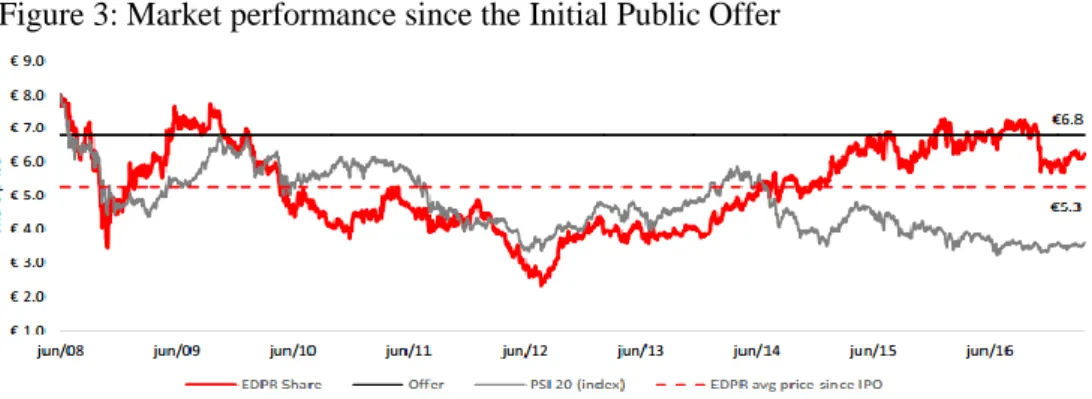
On 4 June 2008, EDPR went public, through an initial public offering (IPO) on the NYSE Euronext Lisbon, by issuing 872,308,162 shares which traded at the initial price of €8.
As at 31March 2017, EDP remains the major shareholder of the company, controlling 77,53% of its capital. EDP is listed in the NYSE Euronext Lisbon since its privatisation in 1997. It is the third largest electric company and one of the main distributors of gas in the Iberian Peninsula. With more than 10 million electricity customers in 14 countries, the company has an installed capacity of 25.2 GW, with 65% of the energy produced in 2016 coming from renewable sources.
The remaining 22.47% are free-float across a wide range of international investors from 23 countries. From these, the biggest stake is owned by MFS Investment Management, controlling 3.11% of EDPR’s capital and voting rights.
26
3.2.3. Company Performance
From the global 10.4 GW portfolio, 10.1 GW are fully consolidated while 356 MW are related to minority equity stakes in projects in Spain and the United States. In 2016, the company installed 770 MW (+8%), 429 MW of them in the US.
In order to minimise the exposure to market volatility, 91% of the installed capacity is backed with long-term contracts with pre-defined remuneration schemes, reaching an average price of €60.5 in 2016 (table 2).
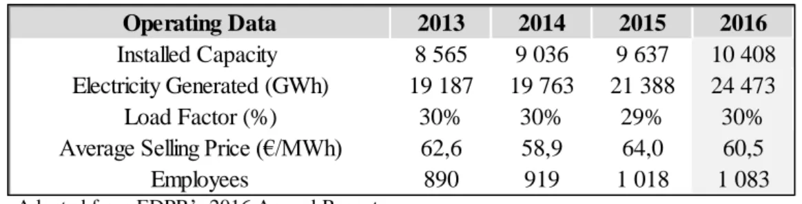
Regarding its operational performance over the year, EDP Renováveis contributed to avoiding over 20 megatons of CO2 emissions by producing 24.5 TWh of renewable energy. A sustained growth strategy and the maintenance of a load factor14 above the market (around 30% over the past years) supports the continuous increase in electricity output.
Regarding the financial performance of EDPR, revenues totalled €m 1,650.8 in 2016 (+6.7%) as a consequence of the increase in total electricity generation (table 3).
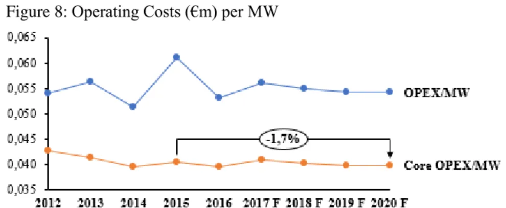
Over the last years, Core OPEX15 per MW has steadily decreased due to firm’s strict control over operational costs, which allowed the company to present strong EBITDA margins, over 70%.
14Load Factor is the ratio of the total energy actually produced in one period over the maximum energy output that could have been produced at full capacity
15 Supplies and Services + Personnel Costs
Financial Data (€m) 2013 2014 2015 2016
Revenues 1 316,4 1 276,7 1 547,1 1 650,8
Operating Costs & Other Operating Income (395,8) (373,5) (404,8) (479,8)
EBITDA 920,5 903,2 1 142,3 1 171,0
EBITDA Margin 70% 71% 74% 71%
EBIT 473,0 422,4 577,8 564,0
Net Financial Expenses (261,7) (249,9) (285,5) (350,1)
Net Profit (Equity holders of EDPR) 135,1 126,0 166,6 56,3 Table 3: EDPR’s Financial Summary 2013-2016
Adapted from EDPR’s 2016 Annual
Operating Data 2013 2014 2015 2016
Installed Capacity 8 565 9 036 9 637 10 408
Electricity Generated (GWh) 19 187 19 763 21 388 24 473
Load Factor (%) 30% 30% 29% 30%
Average Selling Price (€/MWh) 62,6 58,9 64,0 60,5
Employees 890 919 1 018 1 083
Table 2: EDPR’s Operational Summary 2013-2016