D ´ARIO FERREIRA1, SANDRA S. FERREIRA1, C ´ELIA NUNES1 AND JO ˜AO T. MEXIA2
1Department of Mathematics, University of Beira Interior, Covilh˜a, Portugal; 2Department of Mathematics, Faculty of Science and Technology, New University of Lisbon, Monte da Caparica, Portugal
The aim of this article is to present an estimation procedure for both fixed effects and variance components in linear mixed models. This procedure consists of a maximum likelihood method which we call Three Step Minimization, TSM. The major contribu-tion of this method is that when variances tend to be null standard algorithms behave badly, unlike the TSM method, which uses a grid search algorithm in a compact set. A numerical application with real and simulated data is provided.
Keywords Mixed models; Inference; Maximum likelihood; Variance components; Newton-Raphson.
Mathematics Subject Classification 60E05; 62F25.
1 Introduction
The estimation problem of variance components in the case of balanced designs in mixed models has been extensively treated, see for example Khuri and Sahai (1985), Searle (1971) and Searle (1995). Inference becomes less elegant when the orthogo-nality conditions fail to hold.
Prior to the early 1990s, most applications used some version of analysis of vari-ance (ANOVA). The sums of squares for an ANOVA table are easily calculated and are unambiguous, see for example LaMotte (1973) and Vanleeuwen et al (1999). The early development of ANOVA estimation of variance components for unbal-anced data are attributed to Henderson (1953). Nowadays, with the development of computing facilities, the use of maximum likelihood (ML) methods has sparked considerable interest since, despite the methodology for ML estimation is simple, its implementation is mathematically intense. The likelihood function is maximized
Received September 2, 2013
Address correspondence to D´ario Ferreira, Department of Mathematics, University of Beira Interior, Avenida Marquˆes D’ ´Avila e Bolama, 6200 Covilh˜a, Portugal E-mail: [email protected]
over the parameter space under non-negative definite estimates of the variance ma-trices where data is assumed to be normally distributed, see Khuri (1985). Under certain regularity conditions, ML estimators of variance components are consistent, asymptotically efficient and asymptotically normal, see Miller (1977).
Jennrich and Schluchter (1985) and Fairclough and Helms (1986) compared performances of the Newton-Raphson, NR, the Fisher of Scoring method, FS, and the EM algorithm. Lindstrom and Bates (1988) provided arguments favoring the use of the NR method. Based on some starting values for the parameters, procedures based on NR method iteratively update the estimates until convergence is achieved, see Ypma (1995). The difference for the FS is that the FS replaces the observed sec-ond derivatives with its expectation. This method was introduced by Fisher (1925). The NR approach is usually very good if the initial estimate is close to the value of the parameter. But if it is not close enough the iterative process may converge too slowly, may not converge at all or may converge to parameter values on or outside the boundary of the parameter space. This problem might be circumvented by specify-ing better startspecify-ing values or by usspecify-ing other numerical procedures, see Hartley and Rao (1967) or Stern and Welsh (2000). Problems concerning the estimation of variance components in mixed effects models were extensively discussed in the monograph by Demidenko (2013).
In this paper we present a maximum likelihood method for the estimation of both fixed effects and variance components in balanced and unbalanced linear mixed models, which we call Three Step Minimization, TSM. With this approach we first profile out the fixed parameters. Then, after a re-parametrization we switch to using ratio parameters profiling out the variance components. Finally we use a grid search algorithm to carry out a minimization, choosing those ratio parameters that minimize the transformed log likelihood function.
The main advantage of our method is that the grid search is robust and can easily identify variances that are zero or tend to zero. To the contrary, standard algorithms, such as NR or FS, behave badly in this situation. Besides this, TSM is very easy to implement in R software, which is free and available on the internet, and it does not need any starting value, since the grid search will be restricted to the interval [0, 1]. Moreover, our estimates may be used as excellent starting values for the NR method. This article is structured as follows. In the next section we make a brief pre-sentation of linear mixed models. Then we explain how to estimate the parameters through the TSM method. The fourth section provides a numerical comparison of our approach with the NR and FS. Namely we present a numerical example applied to simulated and real data. We used designs with small number of replicates and with one variance component very close to zero, since these are the type of designs we are interested in. Apart from the example in the application with real data this type of de-sign may be used, for example in medicine, in which patients suffer from infrequent pathologies. Finally in the last section we present some comments.
2 Model
Let Y = (Y1, ..., Yn)>describe the observation vector in the linear mixed model
Y = X β + k−1 X l=1
Zlbl+ e, (1)
where X and Zl are known n × m and n × cl matrices respectively, X has full rank, β ∈ Rm is fixed and the random effects b
l and e are assumed to be normally distributed and independent. We put
bl∼ N (0, σl2Icl), (2) l = 1, ..., k − 1 and e ∼ N (0, σ2kIn). (3) Therefore E(Y ) = X β (4) and V (σ2) = V ar(Y ) = k X l=1 σl2Ml, (5) where Ml = ZlZ>
l , l = 1, ..., k − 1, Mk= Inand σ2= (σ12, ..., σ2k)>. Thus we have
Y ∼ N (X β, V (σ2)) (6)
which has density
n(Y |X β, V (σ2)) = e −1
2(Y −X β)>V (σ2)−1(Y −X β)
(2π)n/2p|V (σ2)| . (7)
Having thus the log-likelihood function
l(β, σ2|Y ) = −n 2log(2π) − 1 2log|V (σ 2)| −1 2(Y − X β) >V (σ2)−1(Y − X β), (8)
with |A| describing the determinant of matrix A.
In the next section we will show how to estimate the parameter vector θ = (β, σ2)> using our approach. The description of the NR method may be seen in Demidenko (2013).
3 Three Step Minimization
Maximizing (8) is equivalent to minimizing
l∗(β, σ2|Y ) = log|V (σ2)| + (Y − X β)>V (σ2)−1(Y − X β). (9) We will minimize (9) in three steps. In the first step we will replace the goal function by another which depends only on the variance components. In the second step we replace the goal function depending on the variance components by another which depends on ratio parameters. The third step consists of a numerical minimization.
• First step:
The minimum of l∗(β, σ2|Y ) for a fixed σ2 is obtained for the corresponding least squares estimator
˜ β = ³ X>V (σ2)−1X ´−1 X>V (σ2)−1Y . (10) Thus Y − X ˜β = (In− X (X>V (σ2)−1X )−1X>V (σ2)−1)Y , (11) and moreover (Y − X ˜β)>V (σ2)−1(Y − X ˜β) = Y>PY , (12) where P = V (σ2)−1− V (σ2)−1X (X>V (σ2)−1X )−1X>V (σ2)−1.
So the minimum of l∗(β, σ2|Y ) for a fixed σ2 will be given by the profile log likelihood
l∗∗(σ2|Y ) = log|V (σ2)| + Y>PY , (13) see Pinheiro and Bates (2000). We should point out that now, after profiling out the fixed parameters, the number of variables to be estimated has been reduced substan-tially since we only have to consider σ2.
• Second step:
In the second step we will consider ratio parameters γl, with
γl= σl2
ρ , l = 1, ..., k, (14)
where ρ = Pkl=1σ2
l, profiling out the parameter corresponding to the sum of the variance parameters.
Let us assume that γ = (γ1, ..., γk). Now
V (σ2) = k X l=1 σl2Ml = ρ k X l=1 γlMl= ρV (γ), (15)
with V (γ) = k X l=1 γlMl, l = 1, ..., k. (16) So l∗∗(σ2|Y ) may be rewritten as l∗∗(ρ; γ|Y ) = log(ρn|V (γ)|) + + Y>[1 ρV (γ) −1− 1 ρV (γ) −1X (X>1 ρV (γ) −1X )−1X>1 ρV (γ) −1]Y = nlogρ + log(|V (γ)|) + 1 ρY >[V (γ)−1− V (γ)−1X (X>V (γ)−1X )−1X>V (γ)−1]Y .(17) Thus ∂l∗∗(ρ; γ|Y ) ∂ρ = n ρ − 1 ρ2Y>[V (γ)−1 − V (γ)−1X (X>V (γ)−1X )−1X>V (γ)−1]Y . (18) So, considering Q = Y>[V (γ)−1− V (γ)−1X (X>V (γ)−1X )−1X>V (γ)−1]Y , (19) the minimum for the given γ is attained with
ρ = Q
n. (20)
This minimum will be
l(γ|Y ) = nlog(Q
n) + log(|V (γ)|) + n. (21)
• Third step:
In this step we will minimize the variance-profile log-likelihood function in (21). To do that we take the ratio parameters defined in (14) and use a stochastic or a grid search algorithm to carry out a numerical minimization, choosing those γl, l = 1, ...k, that minimize l(γ|Y ), and complete the adjustment. Note that the γl, l = 1, ..., k will vary in the compact set
D = {γ1, ..., γk}, (22)
where 0 ≤ γl ≤ 1, l = 1, ..., k andPkl=1γl = 1. So this minimization is under constraint of these conditions. In the numerical comparisons we used a grid search algorithm. A brief description of it may be found in the next section. Moreover, the scheme of the grid search algorithm may be seen at
http : //dar364.wix.com/dario]!algorithms/c1oi. Finally there will be
˜
To estimate the remaining parameters we may now use ˜σ2 to obtain V (˜σ2), the estimator of V (σ2), in (5), and then use it in (10) providing
˜ β = ³ X>V (˜σ2)−1X ´−1 X>V (˜σ2)−1Y . (24)
Thus, using the TSM method we are able to estimate the variance components and the fixed effects for an arbitrary model.
4 Numerical application
4.1 Numerical comparison using simulated data
In order to compare the estimates of the variance components obtained through the TSM, and the ones obtained through the NR and FS, using simulated data and with one variance component close to zero, we considered 7 unbalanced models, s = 1, ..., 7. Each model has a three level fixed effects factor, A, that crosses with a two level fixed effects factor, B, which nests an r level random effects factor, C, where r = s + 1. So, the 1-st model is A3× (B2 ⊃ C2), while the 7-th model is
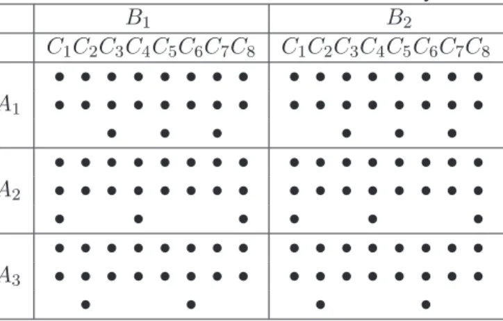
A3× (B2 ⊃ C8). We used these models because they have a combination of nested and crossed effects and are widely used, see for example Khuri et al (1998). Table 1 shows how the data are distributed in the 7-th model, that is, in the case where C factor has 8 levels. The remaining models are obtained by removing levels of the C factor. The table contains dots instead of values because the data were simulated 10000 times.
In Section 4.2 we will use a very similar design to the first one (s = 1) presented in this section. We thought of using this design because so we are replicating the design described in the application to real data. When s=1, the design is almost the same. Thus, this design could be used for the investigation described in the applica-tion to real data but varying the number of clones between 2 (s=1) and 8 (s=7).
The models for the observation vectors Y>
s = (Y1, ..., Yns), s = 1, ..., 7, are given by
Ys= Xsβ + Z1,sb1,s+ Z2,sb2,s+ es (25) where β is a 12 × 1 fixed vector,
b1,s∼ N (0 , σ1,s2 I6(s+1)) b2,s∼ N (0 , σ2,s2 I2(s+1)) es∼ N (0 , σ3,s2 Ins) , (26)
s = 1, ..., 7, are independent and Xs, Z1,sand Z2,sare known design matrices. Let
Table 1: Distribution of observations by factors for the 7-th model. B1 B2 C1C2C3C4C5C6C7C8 C1C2C3C4C5C6C7C8 • • • • • • • • • • • • • • • • A1 • • • • • • • • • • • • • • • • • • • • • • • • • • • • • • • • • • • • • • A2 • • • • • • • • • • • • • • • • • • • • • • • • • • • • • • • • • • • • • • A3 • • • • • • • • • • • • • • • • • • • •
be the vector with the assumed numbers for the variance components and
β¦>= (β1, ..., β12), (28)
where βj = 1, j = 1, ..., 12, be the vector with the assumed numbers for the fixed effects. Note that one of the assumed numbers for the variance components is 0.05.
Hereinafter we used the R software to proceed as follows N = 10000 times:
We simulated Ys, s = 1, ..., 7 with the above assumed numbers for the parame-ters. Then despite the observation vectors and all parameters are known, we assumed that we only knew Ys, Xs, Z1,sand Z2,s, s = 1, ..., 7 and used both methods to esti-mate the parameters and compare the obtained estiesti-mates with the assumed numbers in (27) and (28).
To estimate the parameters using the TSM method we minimized the function in (21) with respect to γs, s = 1, ..., 7. To do that we considered γs= (γ1,s, γ2,s, γ3,s) and used a grid search algorithm, whose scheme is presented at
http : //dar364.wix.com/dario]!algorithms/c1oi. The programmed algorithm for s = 1 is also available. The algorithm makes vary γl,s, l = 1, 2, 3, s = 1, ..., 7,
such that γ1,s= 0.01 × k γ2,s= 0.01 × i × (1 − γ1,s) γ3,s= 1 − (γ1,s+ γ2,s) , (29)
with k = 0, ..., 100 and i = 0, ..., 100, thus having ½
0 ≤ γl,s ≤ 1, l = 1, 2, 3
γ1,s+ γ2,s+ γ3,s= 1 , (30)
s = 1, ..., 7. Proceeding that way it calculated the value of l(γ|Y ), in (21), for each γs and gave us those that minimize l(γ|Y ). Next we obtained the ˜σ2
from (23) and the ˜βs, s = 1, ..., 7, from (24). Note that there is no need to search for a starting value, since our search is restricted to the interval [0, 1].
The idea behind the NR method is to approximate a given function in each iter-ation by a quadratic function and then move to the minimum of this quadratic, see Ypma (1995). The quadratic approximation in a suitable neighborhood of a given point, θ, with components θ1, ..., θw, is given by a second order Taylor expansion
l(θ) ≈ l(θ0) + (θ − θ0)>∂l(θ)∂θ |θ0+ 12(θ − θ0)> µ ∂2l(θ) ∂θi∂θj |θ0 ¶ (θ − θ0). (31)
So, to estimate the parameters using the NR method we minimized the func-tion in (31). To do that we used an algorithm whose scheme is presented at http : //dar364.wix.com/dario]!algorithms/c1oi. For the maximum difference between two successive iterations we considered ² = 0.01. We used this ² to ensure that the conditions were similar for both methods.
To apply the NR method we needed to consider some starting values. We could use an algorithm to select them but as we wanted to study the behavior of the NR with smaller and larger starting values we used the values presented in Table 2. If the starting value is smaller than the assumed number, AN , in (27), we call the NR method NR-L. Otherwise we call it NR-R. For example, if AN = 1, the starting values for NR-L and NR-R methods will be 0.75 and 1.25 respectively.
Table 2: Starting values for NR-L and NR-R.
AN : 0.05 0.5 1
NR-L 0.001 0.25 0.75
NR-R 0.25 0.75 1.25
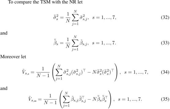
To compare the TSM with the NR let
¯˜σ2 s = 1 N N X j=1 ˜ σs,j2 , s = 1, ..., 7, (32) and ¯˜βs= 1 N N X j=1 ˜ βs,j, s = 1, ..., 7. (33) Moreover let ˜ Vs,¦= N − 11 N X j=1 ˜ σ2s,j(˜σs,j2 )>− N ¯˜σ2s(¯˜σs2)> , s = 1, ..., 7, (34) and ˜ Vs,¦¦ = N − 11 N X j=1 ˜ βs,jβ˜s,j> − N ¯˜βs¯˜βs> , s = 1, ..., 7. (35)
Table 3 shows the obtained values for
d1,s= k¯˜σ2s− σ2¦k, s = 1, ..., 7, (36) and Table 4 shows the obtained values for the trace of matrix ˜Vs,¦, tr
³ ˜ Vs,¦ ´ , s = 1, ..., 7, respectively.
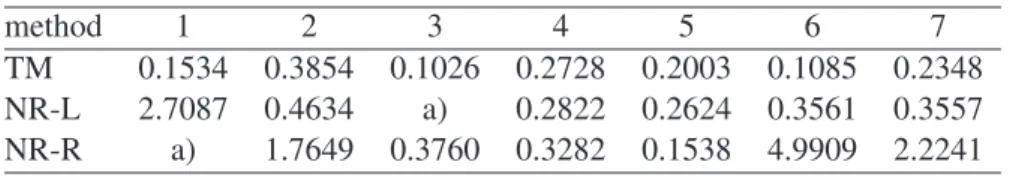
Table 3: Obtained values for d1,s, s = 1, ..., 7.
method 1 2 3 4 5 6 7
TM 0.1534 0.3854 0.1026 0.2728 0.2003 0.1085 0.2348
NR-L 2.7087 0.4634 a) 0.2822 0.2624 0.3561 0.3557
NR-R a) 1.7649 0.3760 0.3282 0.1538 4.9909 2.2241
a) Function in (31) did not converge.
Table 4: Values of tr ³ ˜ Vs,¦ ´ , s = 1, ..., 7. 1 2 3 4 5 6 7 TM 0.0341 0.0536 0.0210 0.0421 0.0209 0.0981 0.0172 NR-L 0.9760 0.0104 a) 0.0708 0.0002 0.1029 0.0772 NR-R a) 18.2697 14.4334 17.0105 0.0221 1.4981 2.0143
a) Function in (31) did not converge.
It may be seen that in general the TSM method gave more accurate values with smaller variation. Moreover, NR-L did not converge when s = 3 and NR-R did not converge when s = 1. Note that both algorithms may be improved. Perhaps using typical algorithms to select starting values would provide a more realistic represen-tation of NR implemenrepresen-tation and performance, while for the TSM we could reduce the net in the compact set. Or alternatively we could have used any other grid search algorithm or even a stochastic algorithm. However our intention was to show that TSM method finds good estimates when the ML solution is on the boundary of the minimization domain and does not require starting values. Moreover, once we have the estimates obtained by the TSM these could also be improved by using them as starting values for the NR. We will see an application of this in Section 4.2.
Table 5 shows the obtained values for
d2,s= k¯˜βs− β¦k, s = 1, ..., 7. (37) and Table 4 shows the obtained values for the trace of matrix ˜Vh,¦¦, tr
³ ˜ Vh,¦¦ ´ , s = 1, ..., 7.
It may be seen that the values of d2,sand tr ³
˜ Vh,¦¦
´
, s = 1, ..., 7 are very similar. Thus, we may conclude that in this case the method used to estimate the variance components does not influence the estimates obtained for β.
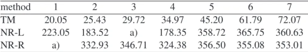
Table 7 shows the sum of the time spent (10.000 cases), in seconds, in obtaining the estimates of the variance components and the fixed effects. It may be seen that
Table 5: Obtained values for d2,s, s = 1, ..., 7.
method 1 2 3 4 5 6 7
TM 2.1284 2.0858 2.1344 2.0424 2.0850 2.1666 2.0855
NR-L 2.1355 2.0807 a) 2.0428 2.0844 2.1666 2.0824
NR-R a) 2.0843 2.1407 2.0449 2.0965 2.1676 2.0962
a) Function in (31) did not converge. Table 6: Values of tr ³ ˜ Vs,¦¦ ´ , s = 1, ..., 7. 1 2 3 4 5 6 7 TM 0.4209 0.7895 0.7967 0.6791 0.1291 0.6820 0.3265 NR-L 0.4275 0.7870 a) 0.6871 0.1133 0.6807 0.3213 NR-R a) 0.7870 0.7869 0.6786 0.1284 0.6808 0.3571
a) Function in (31) did not converge.
Table 7: Sum of the time spent, in seconds, in obtaining the values of ˜σ2and
˜ β. method 1 2 3 4 5 6 7 TM 20.05 25.43 29.72 34.97 45.20 61.79 72.07 NR-L 223.05 183.52 a) 178.35 358.72 365.75 360.63 NR-R a) 332.93 346.71 324.38 356.50 355.08 353.01
a) Function in (31) did not converge.
TSM method took less time than the NR-L and NR-R. However, as the values are all in fractions of seconds we conclude that time is trivial.
Besides this comparison we also estimated the variance components using SPSS software through the FS. To do that we used one of the simulated observation vectors per model. The used observation vectors are available at
http : //dar364.wix.com/dario]!algorithms/c1oi. We used SPSS instead of R software to compare the estimates obtained by our algorithms with estimates ob-tained by an other software. The obob-tained estimates, as well as d1,s, s = 1, ..., 7, are presented in Table 8.
Table 8: Obtained values for d1,s, s = 1, ..., 7, using SPSS software through the FS.
1 2 3 4 5 6 7
d1,s 0.3693 0.4664 0.2522 0.5178 0.3692 0.2630 0.2052
Comparing values in Table 3 and Table 8 we see that, excluding the case where s = 2, s = 4 and s = 5, SPSS through the FS gave more accurate estimates than the R software through our algorithms for NR-L and NR-R. But excluding the case where s = 7, R software through the TSM gave more accurate estimates than the SPSS through the FS.
4.2 Application to real data
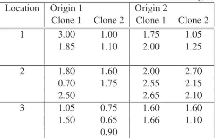
We considered an experiment in which two groups of two clones, grown side by side, of the caste Touriga Nacional. The origins of the two groups were distinct. As before there is a fixed effects factor (location) that crosses with another fixed effects factor (origin) which nests a random effects factor (clone). The yields, in Kg, are presented in Table 9. These data were presented in Fonseca et al. (2003) in an application to a grapevine experiment. Here we introduced imbalance by deleting some observations from the original table. The yields are presented in Table 9.
Table 9: Yields in Kg.
Location Origin 1 Origin 2
Clone 1 Clone 2 Clone 1 Clone 2
1 3.00 1.00 1.75 1.05 1.85 1.10 2.00 1.25 2 1.80 1.60 2.00 2.70 0.70 1.75 2.55 2.15 2.50 2.65 2.10 3 1.05 0.75 1.60 1.60 1.50 0.65 1.66 1.10 0.90
The model for the observation vector Y is
Y = X β + Z1b1+ Z2b2+ e
where β is a 12 × 1 fixed vector, b1 ∼ N (0 , σ12I12) b2 ∼ N (0 , σ22I4) e ∼ N (0 , σ23I28) ,
are independent and X , Z1and Z2are known design matrices.
Using again the R software we obtained the estimates for the variance compo-nents applying the TSM method which are
˜ σ21 = 0.025120 ˜ σ2 2 = 0.000129 ˜ σ2 3 = 0.185249 .
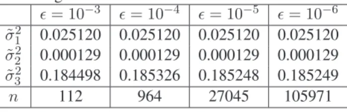
Then we used these values as starting values for The NR and obtained the esti-mates presented in Table 10. We used ² = 10−3, ² = 10−4, ² = 10−5 and ² = 10−6. The number of iterations is represented by n.
Table 10: Obtained estimates for the variance components using the TSM estimates as starting values for the NR.
² = 10−3 ² = 10−4 ² = 10−5 ² = 10−6 ˜ σ12 0.025120 0.025120 0.025120 0.025120 ˜ σ2 2 0.000129 0.000129 0.000129 0.000129 ˜ σ2 3 0.184498 0.185326 0.185248 0.185249 n 112 964 27045 105971
Comparing these results from those obtained through the TSM method we see that the estimates for σ21 and σ22 obtained using the NR were identical to those ob-tained through the TSM, irrespective of the number of iterations. Besides this the es-timate for σ2
3 obtained using the NR started by diverging from that obtained through the TSM, but with the increase of iterations these approached. Thus we may conclude that the estimates obtained through the TSM were validated by the NR.
We also obtained the variance components estimates through the NR and FS, using SPSS software, which are presented in Table 11. We used ² = 10−8.
Table 11: Obtained estimates for the variance components through the NR and FS using SPSS software. NR FS ˜ σ2 1 0.027759 0.027759 ˜ σ2 2 0 0 ˜ σ32 0.183873 0.183873
It may be seen that the estimates obtained by SPSS through the NR and FS are very close to the ones obtained by the TSM and the NR with the TSM estimates as starting values. So, once again, we may conclude that the estimates obtained by our algorithms were validated by SPSS through the NR and FS.
5 Final Comments
We proposed a maximum likelihood method, the TSM method, for the estimation of both fixed effects and variance components in balanced and unbalanced mixed models.
A numerical comparison with the NR and FS was provided. In general the TSM method gave more accurate values than the NR. As stated before, we could use an algorithm to select the starting values for the NR but as we wanted to study the be-havior of the NR with smaller and larger starting values we used the values presented in Table 2. These are for sure not the best starting values for the NR but note that the TSM method can also be improved by making the net narrower in step 3. Comparing with the FS method, the TSM method obtained more accurate results than the FS
in six of seven cases. The FS method was more accurate than the TSM for s = 7, obtaining d1,2 = 0.2052, while with the TSM method the result was d1,2 = 0.2348. Despite the added value of this comparison, we think that the major contribution of the TSM method is that when variances tend to be null, i.e. the ML solution is on the boundary of the minimization domain, standard algorithms, such as NR or FS, behave badly, unlike the TSM method, which uses a grid search in the compact set [0, 1]. In addition, TSM does not need a starting value. So, in this sense, this method proves easier and faster to apply than the Newton Raphson. Besides this, TSM is very easy to implement in R software, which is free and available on the internet.
Acknowledgements
The authors gratefully acknowledge the reviewers for their very valuable comments.
This work was partially supported by the Center of Mathematics, University of Beira Interior through the project PEst-OE/MAT/UI0212/2014 and by CMA, Faculty of Science and Technology, New University of Lisbon, through the project PEst-OE/MAT/UI0297/2011.
References
Demidenko, E. (2013). Mixed Models: Theory and Applications with R, 2nd Edition. Wiley, New York.
Fairclough, D. L., Helms, R. H. (1986). A mixed linear model with linearcovariance struc-ture: a sensitivity analysis of maximum likelihood estimators. J. Statist. Comput. Simula-tion. 25: 205–236.
Fisher, R. A. (1925). Methods for Research Workers. Oliver and Boyd, Edimburgh. Fonseca, M., Mexia, J. T., Zmy´slony, R.(2003). Estimating and Testing of Variance
Compo-nents: An Application to a Grapevine Experiment. Biometrical Letters 40(1):1–7. Hartley, H., Rao, J. (1967). Maximum-Likelihood Estimation for the Mixed Analysis of
Variance Model. Biometrika. 54(1/2): 93–108.
Henderson, C. (1953). Estimation of variance and covariance components. Biometrics. 9: 226–252.
Jennrich, R. I., Schluchter, M. D. (1985). Unbalanced repeated-measures models with struc-tured covariance matrices. Biometrics. 42: 805–820.
Khuri, A., Sahai, H. (1985). Variance components analysis: a selective literature survey. International Statistical Review. 53: 279-300.
Khuri, A., Mathew, T. and Sinha, B. (1998). Statistical Tests for Mixed Linear Models Wiley, New York.
LaMotte, L. R. (1973). Quadratic Estimation of Variance Components. Biometrics. 29(2): 311–330.
Lindstrom, M., Bates, D. (1988). Newton-Raphson and EM algorithms for linear mixed
effects models for repeated measures data. J. Am. Statist. Assoc. 83: 1014–1022.
Miller, J. J. (1977). Asymptotic properties of maximum likelihood estimates in the mixed model of the analysis of variance. Ann. Stat. 5: 746–762.
Pinheiro, J., Bates, D. (2000). Mixed Effects Models in S and S-Plus. Springer, New York. Searle, S. (1971). Topics in variance component estimation. Biometrics. 27: 1–76. Searle, S. (1995). An overview of variance component estimation. Metrika. 42: 215–230. Stern, S., Welsh, A. (2000). Likelihood Inference for Small Variance Components. Can. J.
Stat. 28(3): 517–532.
Ypma, T. (1995). Historical Development of the Newton-Raphson Method. SIAM Review. 37(4): 531–551.
Vanleeuwen, D., Birkes, D., Seely, J. (1999). Balance and Orthogonality in Designs for Mixed Classification Models. Ann. Stat. 27(6): 1927–1947.