Todos os direitos reservados.
É proibida a reprodução parcial ou integral do conteúdo
deste documento por qualquer meio de distribuição, digital ou
impresso, sem a expressa autorização do
REAP ou de seu autor.
The Effects of Gender Segregation at the
Occupation, Industry, Establishment, and Job-Cell
Levels on the Male-Female Wage Gap
Miguel Nathan Foguel
The Effects of Gender Segregation at the Occupation, Industry,
Establishment, and Job-Cell Levels on the Male-Female Wage Gap
Miguel Nathan Foguel
The Effects of Gender Segregation at the Occupation,
Industry, Establishment, and Job-Cell Levels on the
Male-Female Wage Gap
Miguel Nathan Foguel
IPEA
November 9, 2015
First Version
Abstract
1
Introduction
Gender differences in wages have declined in many countries in recent decades but they are still a persistent phenomenon (Blau and Khan, 2003; ˜Nopo et al., 2011). Understanding why women consistently earn less than men is essential to enrich our knowledge on the channels that feed this persistent wage gap. This paper focuses in one the channels empha-sized by previous research: the effect that the gender segregation in occupations, industries, establishments, and job cells (i.e. occupations within establishments) has on the gender pay gap.
There are various theories that explain why there are gender differences in the labor market. On the supply side, the human capital model (Mincer and Polachek, 1974) offers an explanation based on different decisions made by males and females in the acquisition of human capital. Given women’s more intermittent attachment to the labor market, their op-timal response is to acquire less education and labor market experience. The human capital model (Polachek, 1981) also predicts that women choose occupations that require substan-tially less investment in on-the-job training and whose rates of depreciation for periods out of the labor force are lower. One of the main implications of the human capital model is that part the sex pay gap can be explained by gender differences in productivity-related at-tributes. The human capital model also helps explaining the process of allocation of women across the different types of occupations and jobs.
Closely related to the human capital model are the arguments bases on gender differences in preferences and comparative advantages. To the extent that men and women differ in their preferences for job attributes (e.g., flexible vs. rigid work schedules, safe vs. hazardous jobs) and in comparative advantages in performing distinct tasks (e.g., requiring more or less physical strength or caring), males and females tend to be differently sorted across occupations, industries, firms, and jobs. If women value more flexible and “friendlier” jobs than men, the theory of compensating differentials, whereby employers and workers establish a trade between pecuniary and nonpecuniary aspects of the jobs, predicts that females will be more concentrated in lower-paid jobs (Reilly and Wirjanto, 1999a,b).
in firms.
Demand-side explanations mainly stem from models of labor market discrimination. Becker (1971) and Arrow (1973a,b) propose models where discriminatory tastes by em-ployers, employees, or customers lead to sex segregation at the firm level and to a wage differential between (equally productive) men and women. The theory of statistical discrim-ination (e.g., Phelps, 1972; Arrow, 1973b), whereby employers form different beliefs about the distribution of skills between the genders, also predicts the existence of a sex wage dif-ferential. Discriminatory promotion practices has also been proposed as an explanation to the gender segregation and the wage differentials observed in top-ranked positions within firms (Baldwin et al., 2001; Ramsom and Oaxaca, 2005, Coelho et al., 2013).
The main lessons learned from these theories are that, while part of the wage gap is attributable to human capital differences between the genders, the process of allocation of males and females in the labor market leads to a type of sorting in which women end up relatively more concentrated in occupations, industries, firms, and occupations within establishments (job cells) that pay lower wages. This implies that empirical analyses of the determinants of the sex pay gap should take into account not only the human capital differences between the genders but also the patterns of female segregation along these dimensions. Another implication of these theories for empirical work is that unobserved (to the analyst) characteristics of workers and firms play crucial roles as determinants of wages and the sorting process of males and females in the labor market. Lack of control for unmeasured traits of workers and firms may thus generate serious biases in the estimates of the effects of gender segregation on the wages of males and females, and therefore on the gender wage gap.
The importance of female segregation in the labor market has been recognized by many empirical studies of the gender pay gap. Most previous research has focused only on the impact of a single dimension.1 Only Groshen (1991), Bayard et al. (2003), Gupta and
Rothstein (2005), and Amuedo-Dorantes and la Rica (2005) have investigated the effects of segregation at the occupation, industry, establishment, and job-cell levels in the same analysis. However, all these studies suffer from important data limitations: either they covered a limited set of industries and occupations or the data were based on samples of larger firms and few workers per firm. In addition, their wage regressions were all based on
cross-section data. As discussed above, the non incorporation of unobserved heterogeneity into the analysis may render misleading estimates of the wage effects of female segregation along the dimensions of interest.
To tackle these problems, in this paper we rely on a large panel of matched employer-employee data. Based on administrative files maintained by the federal government in Brazil (Rela¸c˜ao Anual de Informa¸c˜oes Sociais - RAIS), the data provides information on every single employment relationship that all registered employers have during the year. The data set is rich in that it contains information on wages and on the characteristics of workers (sex, age, education), establishments (industry, size), and jobs (occupation, tenure). Its census nature allows precise computations of the share of women within the segregation dimensions of interest: occupation, industry, establishment, and job cell (i.e., occupation within establishment). This a strength of this study as compared to the previous literature, which had to rely on small samples of workers or a limited set of occupations to calculate the proportion of females along these dimensions. The longitudinal aspect of the data for workers and establishments also allows us to deal with distinct forms of unobserved heterogeneity in wage regressions. One of the main contributions of this paper is the incorporation of fixed effects for workers, firms, and workers-firms matches in the estimation of the segregation effects of interest on the gender wage gap. To the best of our knowledge, this is the first paper that does that in the literature.2
This paper is structured as follows. In section 2, we describe the the data in more detail and present descriptive statistics. In section 3, we present the various fixed effects models we use to estimate the gender segregation effects of interest as well as their contribution to sex wage gap. Section 4 presents the fixed effect results and compare them to the OLS case. In section 5, we present our main conclusions.
2
Data and Descriptive Statistics
2.1
Data and Variables
The data source employed in this study (Rela¸c˜ao Anual de Informa¸c˜oes Sociais - RAIS -Annual Social Information Report) is a large scale administrative database that contains matched employer-employee information obtained from mandatory reports that are sent annually to the federal government by all registered employers in Brazil. The data set provides information on every single labor contract the employers have with their employees
during the year. For each observation, there is information on the worker’s sex, age, schooling level, month of hiring and displacement at the establishment, occupation, and monthly wages. In addition, the industry and municipality where the establishment is located are also informed. Unique identification numbers for workers and establishments allow us to follow them over the years.
The information on the workers’ wage is used by the federal government to implement a long-standing social program called Abono Salarial (Wage Bonus).3 Given that individual
workers are the beneficiaries of the program, employers ought to be careful in providing the wage information to the government. In this sense, we should expect to find less measurement error in wage data from RAIS than in wages informed by workers in household surveys.
We use data for the years 2003 to 2007. During this period, the database provided information on around 47 million employment relationships for each year, corresponding to 40 million workers and 2.5 million establishments. Due to this huge size, we selected a 1% random sample of all workers whose records appeared inRAIS during this five years period. The procedure generated a sample of 1,174,920 workers who were followed throughout this period. A subset of workers (42.8%) were not observed for the whole period, so our sample is unbalanced.
We imposed a set of filters on the raw sample. First, we dropped observations for all individuals who were younger than 25 or older than 65 years old during the period of analysis. Second, we excluded workers from the agriculture sector. Finally, we deleted all workers for whom the information on the wage, the age, the industry or the occupation was missing in the database. Our final sample has 599,232 workers, 383,360 establishments, 900,176 worker-establishment job matches, and 2,255,290 observations in total.
The wage information available in the data set is the average monthly wage paid to the worker by his/her employer within the year.4 In regressions, we use the logarithm of
the real average monthly wage, which was deflated by the Amplified National Consumer Price Index (IPCA). We also constructed variables for the workers’ general experience in the labor market (measured as age - education - 7), tenure in the same establishment, and whether the establishment was small (less than 9 workers). Our measure of gender segregation is the percent female in a worker’s occupation, industry, establishment, and job cell (occupation within an establishment). It is important to note that it was calculated for all four dimensions before we took the sample, so it is not subject to the type of measurement
3Workers who are paid on average less than two minimum wages during a year are entitled to receive a yearly wage bonus (equivalent to one minimum wage) through this program.
error typically found in other studies that used small samples of workers per establishment. This is particularly important for percent female within job cells, which is the narrowest dimension. The occupation structure was disaggregated in 185 categories, while the industry dimension in 25 categories.
2.2
Descriptive Statistics
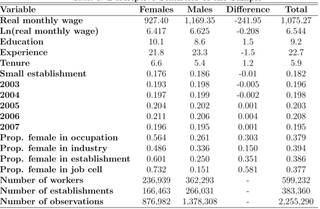
Table 1 exhibits descriptive statistics for the sample used in estimation. Column 2 and 3 display the average characteristics for females and males, while column 4 presents the raw difference between the groups. The last column provides the average values for the whole sample. Estimation is based on information on 236,939 females (876,982 observations over the 2003-2007 period) and 362,293 males (1,378,308 worker-year observations). Women worked at 166,463 different establishments, while men at 266,031.
Table 1: Descriptive Statistics of the Sample
Variable Females Males Difference Total
Real monthly wage 927.40 1,169.35 -241.95 1,075.27
Ln(real monthly wage) 6.417 6.625 -0.208 6.544
Education 10.1 8.6 1.5 9.2
Experience 21.8 23.3 -1.5 22.7
Tenure 6.6 5.4 1.2 5.9
Small establishment 0.176 0.186 -0.01 0.182
2003 0.193 0.198 -0.005 0.196
2004 0.197 0.199 -0.002 0.198
2005 0.204 0.202 0.001 0.203
2006 0.211 0.206 0.004 0.208
2007 0.196 0.195 0.001 0.195
Prop. female in occupation 0.564 0.261 0.303 0.379
Prop. female in industry 0.486 0.336 0.150 0.394
Prop. female in establishment 0.601 0.250 0.351 0.386
Prop. female in job cell 0.732 0.151 0.581 0.377
Number of workers 236,939 362,293 - 599,232
Number of establishments 166,463 266,031 - 383,360
Number of observations 876,982 1,378,308 - 2,255,290
Notes: Means and totals are reported. Wage data in 2007 R$, deflated by the Amplified National Consumer Price Index (IPCA). Education, experience, and tenure are measured in years. Small establishment refers to the proportion of workers employed in establishments with less than 9 employees. Source: Based on microdata fromRela¸c˜ao Anual de Informa¸c˜oes Sociais - RAIS.
The data show that the log wage differential between females and males is .208, or 18.8% (20.7%) in terms of geometric (arithmetic) means.5 Females are considerably more
educated and accumulate far more experience with the same employer than their male counterparts (1.5 years, or 16.9%, and 1.2 years, or 21.3%, respectively). However, they have less labor market experience than men (-1.5 years, or -6.3%). Males are slightly more likely to hold jobs in small establishments than females. These figures reveal that there are important differences in productivity-related characteristics between the two groups. As expected from our sampling scheme, females and males are homogeneously distributed over the sample period.
Looking at the gender segregation patterns, Table 1 confirms what has been observed in other studies: women work in predominantly female occupations, industries, establishments, and job cells; the opposite applies to males. Also similar to other studies, job cells are the most segregated dimension: a random female worked in a job cell that was 73% female, while the average male worked in a job cell that was 15% female.6 Establishment segregation is also
high in our data (the percentage of females is 60% for women and 25% for men), followed by occupation segregation (56% for women and 26% for men) and industry segregation (49% for women and 34% for men). If this elevated degree of female segregation comes from a process through which (observationally equivalent) males and females are sorted in occupations, industries, establishments, and job cells that pay average lower wages and are predominantly female, we should observe a negative effect of these forms of segregation on the wages of both groups. In addition, if this effect is higher for females than for males, it will be responsible for at least part of the gender wage gap we observe in the data.
3
Methods
In this section we present the fixed effect models that control for different types of unobserved heterogeneity associated with the workers, establishments, and worker-establishment job matches. The model framework is inspired by Abowd et al. (1999) and Abowd et al. (2002), who proposed methods for estimating wage regressions in the presence of both worker and firm fixed effects. The actual estimation of the wage regressions is based on Andrews et al. (2005, 2006) and Cornelissen (2008).
We assume that wages are a linear function of observed and unobserved characteristics of workers and establishments. Our interest falls on the effect of female segregation on wages
(.224 log points) but smaller than that found for Denmark in 1995 by Gupta and Rothstein (2005) (.341 log points) and for the U.S. in 1990 by Bayard et al. (2003) (.375 log points). The log wage differential for the U.S. found by Groshen (1991) varied from .240 to .469 depending on the industry and year of analysis.
in four dimensions: occupation, industry, firm, and job cell. One of the contributions of this paper is the estimation of these effects including fixed effects to control for unobserved, time-invariant characteristics of workers, firms, and worker-firm matches. The workers’ fixed effects capture unobserved heterogeneity in their abilities/skills, motivation, preferences, and personality traits, all of which affect wages and can be correlated with the allocation of workers across the four dimensions of interest. If females’ tastes are such that they are prepared to trade more easily the pecuniary for non-pecuniary aspects of the jobs, one should expect to observe a higher concentration of women in occupations, industries, establishment, and job cells that pay lower wages. It could also be that less productively able men and women sort (or are sorted) into predominantly female jobs that command lower wages. In both cases, the estimates of the effects of female segregation on wages will be misleading if worker-specific fixed effects are not part of the model.
On the firms’ side, the fixed effects absorb unobserved heterogeneity in a large set of factors such as their management productivity, discrimination practices, technologies, job attributes, work conditions, and compensation policies. All these dimensions can affect gender sorting across establishments. If females are more frequently hired to work at es-tablishments that pay lower wages, unless establishment fixed effects are controlled for, a negative relationship between wages and female segregation is likely to appear in the data. In one specification of the model, we use a job-match fixed effect which is intended to capture unobserved heterogeneity in worker-firm matches. This specification is quite rich in that it captures the “quality” of the match between the unobserved characteristics of the workers (job preferences, abilities/skills, etc.) and firms (job characteristics, work conditions, etc.). In addition, job match quality also captures the production complementarities between the worker and the firm (Woodcock, 2007). As shown by Woodcock (2008), the quality of job matches is important for wage determination. If the sorting process of workers in the labor market is correlated with differences in job characteristics and match-specific productivity, “good” and “bad” matches can influence not only gender segregation across firms but also across industries and even occupations.7 Thus, controlling for match-specific fixed effects
should absorb at least part of the influence of gender segregation on the wages.
Though included in the wage regressions, the worker-, the establishment-, or the match-specific fixed effects only serve as controls. This is mainly due to the fact that our observation window is relatively short (5 years), so the worker (or match) fixed effects will be incon-sistently estimated. Also, the consistency and precision of the establishment fixed effects depend on the number of workers that join or leave the establishments. While many
lishments display a large number of hirings and displacements, there is a large set of firms (specially the small ones) for which there is little or no worker mobility in our sample.
Since some models include fixed effects for workers, we cannot follow the literature in using a single wage equation for both sexes including a dummy variable for females. Instead, we estimate one equation for each gender and use the difference in intercepts as the measure of the “pure” female-male wage differential, that is, the wage gap that remains after con-trolling for the observable and unobservable characteristics of workers and establishments. The general regression equation we consider is:
ygij(i,t)t =αg+x′ijg(i,t)tβg+θig+ψjg(i,t)+εgij(i,t)t, (1)
where g = m, f denotes males and females, respectively. Workers are indexed by i = 1, ..., Ng, and j(i, t) = 1, ..., J corresponds to the establishment that worker i is employed
at time period t = 1, ..., Ti. The response variable y is the natural logarithm of the real
wage, αg denotes the intercept, x is a vector of time-varying observable characteristics of the worker and the firm, and βg is a conformable coefficient vector. The components θg i
and ψjg(i,t) represent worker-specific and establishment-specific fixed effects which capture unobserved, time-invariant characteristics of workers and establishments, respectively.8 The
mean zero disturbance term ε is assumed to be strictly exogenous with variance clustered at the individual or firm level.
Equation (1) is estimated through three different specifications. The first is pooled OLS where no fixed effects are considered in estimation. This is equivalent to assuming that θgi = ψgj(i,t) = 0, an assumption that can produce the usual omitted variable bias in the estimation of the returns to observable characteristic.9
In the second specification, we only allow for the presence of the establishment-specific fixed effect ψjg(i,t), while in the third we only include the worker-specific effect θgi. These two specifications can be easily estimated through within-group transformations that use time-demeaning of the data at the establishment or the worker level respectively. While still subject to omitted variable biases, the results obtained from these two specifications allow us to have an idea of the separate impact of omitting each component at a time.
We also estimate a model that treats each worker-firm combination as a unique
employ-8Since the equation is estimated separately by gender, it is implicitly assumed that the establishment fixed effects vary between males and females. This assumption allows the unobserved, time-invariant char-acteristics of the establishments to play a separate role in the wage determination process of the genders.
ment match or “spell”. The equivalent equation for this model is written as:
yijg(i,t)t =αg+x′ijg(i,t)tβg+φgij(i,t)+εgij(i,t)t, (2)
where φgij(i,t) represents the match-specific fixed effect between worker i and establishment j where the worker was employed at time t. This term, which can be swept out by a within transformation of data at the job-match level, captures all time-invariant heterogeneity of the particular match between a certain worker and a certain establishment. As mentioned before, this component can be seen as the unmeasured quality of the match formed between the worker and the establishment.10
The last specification we estimate is the two-way fixed effect model where the worker-and the establishment-specific fixed effects are simultaneously included in the wage equation (1). Given the high dimensionality of these two terms when large samples of workers and establishments are used, the conventional least square dummy variable method is not feasible in practice since it requires inverting huge matrices. Hence, one needs to rely on alternative methods to estimate the model. There are essentially two broad strategies to accomplish that. The first is restricting the sample only to workers that remain in the same firm over time. In this case, a simple within-group transformation at the worker level sweeps out both unobserved heterogeneity terms in equation (1). We do not pursue this strategy here.
The second strategy uses all workers and firms in the sample. Since there is no direct within-group transformation that can make the two fixed effects vanish simultaneously, some other method must be used. Abowd et al. (1999) propose approximate statistical methods to the full least square solution, whereas Abowd et al. (2002) provide an exact solution through an interactive conjugate gradient technique that benefits from the existence of sparse matrices in the structure of the normal least square equations. Andrews et al.(2006) propose a method named FEiLSDVj in which workers’ fixed effects are firstly removed through time-demeaning of data over workers (this is the FEi part) and then the model is estimated via least squares with establishment dummies included in the equation (this is the LSDVj part). This method is appropriate for samples where the number of firms is not too large, which is not our case. Here, we follow the method proposed by Cornelissen (2008), which combines features of Andrews et al. (2006) and Abowd et al. (2002). Specifically, the method first uses the within transformation to eliminate the worker fixed effects and then explores the
existence of sparse matrices in the model structure to construct the matrices that belong to the system of normal equation.11 Like Andrews et al. (2006) and Abowd et al. (2002), this
method also delivers the exact least square solution.12
We use the estimates of αg and βg, g = m, f, from equations (1) and (2) to compute the Oaxaca (1973)-Blinder(1973) decomposition of the gender wage gap when fixed effects are included in the model. Specifically, from equation (1) and (2), the raw wage differential between females and males can be decomposed respectively as:
yf −ym = [ˆαf −αˆm] + [x′fβˆf
−x
′mˆ
βm] + [θf −θ
m
] + [ψf −ψ
m
], (3)
and
yf −ym = [ˆαf −αˆm] + [x′fβˆf
−x
′mˆ
βm] + [φf −φ
m
], (4)
where the overbars denote raw sample means and hats represent estimated parameters. The first term in brackets corresponds to the difference between the estimated intercept for each gender equation. It captures the remaining sex differences in wages after controlling for our measures of female segregation and other observable and unobservable characteristics of workers and establishments. The second term is the component attributable to observable time-varying characteristics of workers and firms, including our segregation variables of interest. The last two terms in (3) are the components of the raw wage gap due to differences in the average worker and establishment fixed effects between the genders. The last term in (4) refers to the difference in the average job-match fixed effects. We estimate the model normalizing each average to zero (i.e., θf = θm = ψf = ψm = 0 for equation (3) and φf = φm = 0 for equation (4)), so these components have no contribution to the wage decompositions.13
11It is worth mentioning that there is also another method proposed by Guimaraes and Portugal (2010). We also used this method and obtained identical results (apart from the intercept, which is not estimated in the latter method).
12Though we are not interested in estimating the worker and the firm fixed effects, it is worth noting that their identification depend on the pattern of worker mobility across firms. As shown by Abowd et al. (2002), the identification of these effects can be attained by using methods of graph theory to determine the groups of workers and firms that are connected. A single connected group is formed by all workers who have ever worked for any of the firms in the group during the observation window and all the firms for which any of the workers have ever worked. This implies that a worker in a group cannot have ever worked for a firm in another group and a firm in a group cannot have ever hired a worker from another group. Any firm that has not experienced any worker mobility as well as any worker that has only been employed in a single firm during the sample period do not belong to a connected group. These firms and workers belong to a “non-mover” group. In a labor market with some worker mobility there will be a stratification of workers and firms inP groups. IfNp and Jp are respectively the number of workers and firms in each groupp= 1, ..., P, it is possible to identify (Np−1) + (Jp−1) worker and firm effects within each group.
Following the usual Oaxaca/Blinder decomposition, the second term in (3) and (4) can be further decomposed into components attributable to differences in characteristics between the groups and differences in the “returns” to these characteristic. There are at least two ways to express this extended decomposition depending on the group chosen to be the reference. If males are used as the reference group, the decomposition can be written as:14
yf −ym = [ˆαf −αˆm] + [xf
−xm]′βˆm+ [ ˆβf −βˆm]′xf. (5)
and if females are the chosen group:
yf −ym = [ˆαf −αˆm] + [xf
−xm]′βˆf + [ ˆβf −βˆm]′xm, (6)
These two ways of expressing the decomposition can potentially deliver different results, so we compute both of them.
4
Results
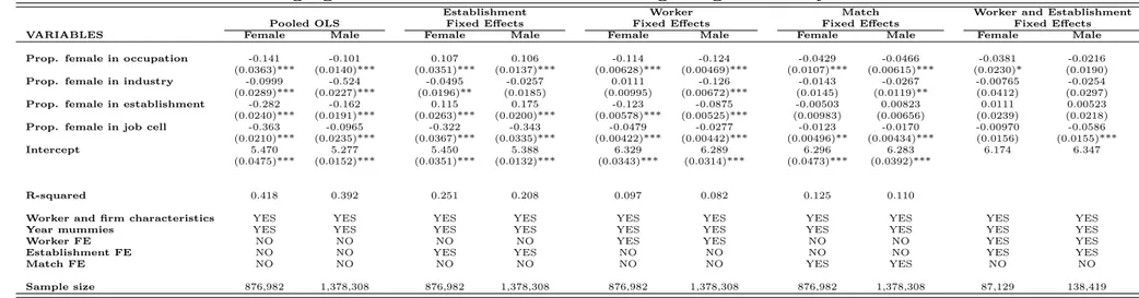
Table 2 presents the results of the wage regressions for all models we estimate. Each pair of columns shows the results for females and males within each model specification (pooled OLS, only establishment fixed effects, only worker fixed effects, only spell/match fixed ef-fects, and worker and establishment fixed effects).15 All models were estimated including
education, a quadratic in experience and in tenure, a dummy for small establishments (nine or less employees), and year dummies.16 We only present the estimates of the effects of the
segregation measures and of the intercepts but the complete set of results are available upon request.
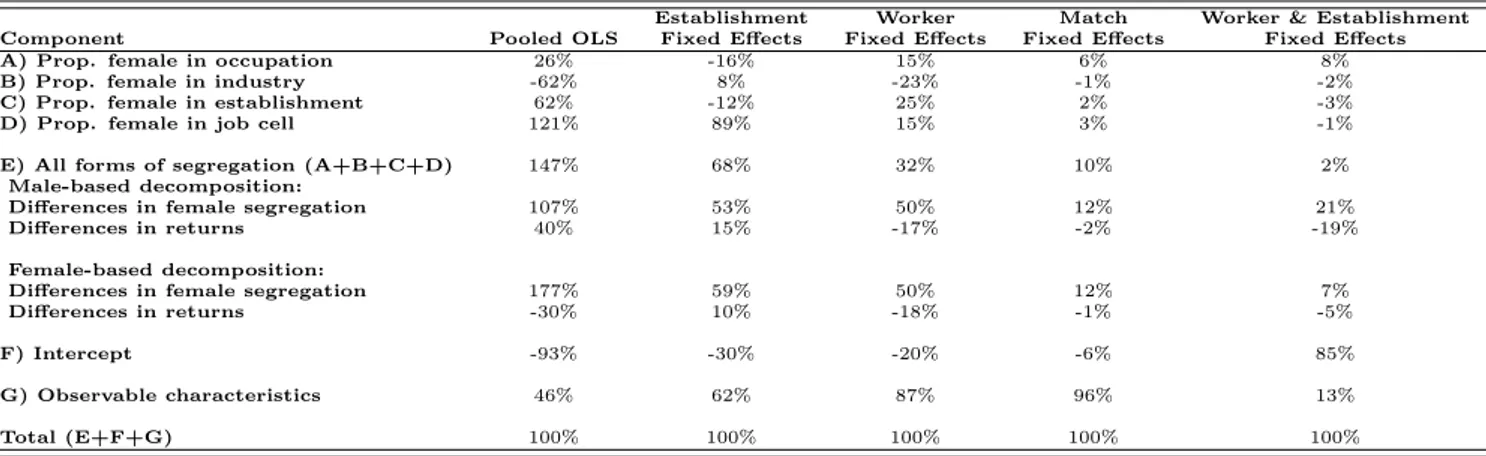
Table 3 reports the results of the Oaxaca/Blinder decomposition of the female/male log wage gap. Together with the portion of the gap attributable to the sex of the worker (i.e., the difference in intercepts between the female and the male regressions), only the results for the contributions of the four segregation measures are exhibited.17 The relative
and (4) to be interpreted as the difference in the controlled mean wages between the gender groups. 14Given our normalization of the average worker, establishment, and match fixed effects, they are not presented in the following expressions.
15Because the estimation of the last model is very slow, it was estimated on a 10% sample of workers used in the previous models.
16Though some models include worker fixed effects, we did not drop the education variable because some workers (specially the younger) change their schooling level along the five years of analysis.
contribution of differences in the average percent female between the sexes and their returns are also presented for the male- and female-based decompositions (equations (5) and (6)).
Beginning with the pooled OLS results, it can be seen from Table 2 that all coefficients estimates of the percent female variables are statistically significant. As found in Groshen (1991), Bayard et al. (2003), and Amuedo-Dorantes and la Rica (2005), the segregation of women at the occupation, industry, establishment, and job-cell levels has a negative effect on the wages of both sexes.18 With the exception of the industry dimension, males’ wages
are more adversely affected than females’ wages by all forms of segregation. The difference in intercepts shows a higher average wage for women after controlling for the segregation measures and the observable characteristics of workers and establishments.
Applying the pooled OLS results into the Oaxaca/Blinder decomposition, Table 3 shows that all but the industry segregation dimension widen the wage gap. The contribution of percent female within job cells is the highest one, followed by the contributions of establish-ment and occupation segregation; the contribution of segregation at the industry level has the opposite sign but the same magnitude of establishment segregation.19 The difference
in the intercepts favoring women implies that the female/male wage gap is shrunk by the individual worker’s sex. Since all other studies that control for the four segregation mea-sures have found that the sex of the worker contributes to widen the gender wage gap, this is a somewhat striking result. Of course, this disparity could be explained by differences in samples, regression specifications, and control variables used in this and the other studies. On a more substantive level, however, the OLS results suggest that the process of sorting of workers and the resulting segregation of women in the Brazilian labor market plays a much higher role than in other countries. We now turn to check the robustness of the pooled OLS results to the inclusion of worker, establishment, and match fixed effects in the model.
There are noticeable changes when establishment fixed effects are incorporated into the model. As displayed in Table 2, although most estimates keep being significant on statistical grounds (the only exception is the effect of industry segregation for males), the sign and magnitudes of coefficient estimates differ from those of the pooled OLS. There is a flip in sign for both males and females in the effect of women segregation at the occupation and establishment levels. The effect of job cell segregation is still negative but has become stronger in absolute value for males, whereas the effect of industry segregation has been
18For the equivalent specification of Gupta and Rothstein (2005), the coefficients estimates of the gender segregation effects are positive either for the occupation or the industry or the establishment levels. The effect of job-cell segregation is always negative though.
Table 2: Segregation Coefficient Estimates of Wage Regressions by Model
Establishment Worker Match Worker and Establishment
Pooled OLS Fixed Effects Fixed Effects Fixed Effects Fixed Effects
VARIABLES Female Male Female Male Female Male Female Male Female Male
Prop. female in occupation -0.141 -0.101 0.107 0.106 -0.114 -0.124 -0.0429 -0.0466 -0.0381 -0.0216 (0.0363)*** (0.0140)*** (0.0351)*** (0.0137)*** (0.00628)*** (0.00469)*** (0.0107)*** (0.00615)*** (0.0230)* (0.0190)
Prop. female in industry -0.0999 -0.524 -0.0495 -0.0257 0.0111 -0.126 -0.0143 -0.0267 -0.00765 -0.0254 (0.0289)*** (0.0227)*** (0.0196)** (0.0185) (0.00995) (0.00672)*** (0.0145) (0.0119)** (0.0412) (0.0297)
Prop. female in establishment -0.282 -0.162 0.115 0.175 -0.123 -0.0875 -0.00503 0.00823 0.0111 0.00523 (0.0240)*** (0.0191)*** (0.0263)*** (0.0200)*** (0.00578)*** (0.00525)*** (0.00983) (0.00656) (0.0239) (0.0218)
Prop. female in job cell -0.363 -0.0965 -0.322 -0.343 -0.0479 -0.0277 -0.0123 -0.0170 -0.00970 -0.0586 (0.0210)*** (0.0235)*** (0.0367)*** (0.0335)*** (0.00422)*** (0.00442)*** (0.00496)** (0.00434)*** (0.0156) (0.0155)***
Intercept 5.470 5.277 5.450 5.388 6.329 6.289 6.296 6.283 6.174 6.347
(0.0475)*** (0.0152)*** (0.0351)*** (0.0132)*** (0.0343)*** (0.0314)*** (0.0473)*** (0.0392)***
R-squared 0.418 0.392 0.251 0.208 0.097 0.082 0.125 0.110
Worker and firm characteristics YES YES YES YES YES YES YES YES YES YES
Year mummies YES YES YES YES YES YES YES YES YES YES
Worker FE NO NO NO NO YES YES NO NO YES YES
Establishment FE NO NO YES YES NO NO NO NO YES YES
Match FE NO NO NO NO NO NO YES YES NO NO
Sample size 876,982 1,378,308 876,982 1,378,308 876,982 1,378,308 876,982 1,378,308 87,129 138,419 Notes: Standard errors reported in parentheses and adjusted for clustering at the establishment level. All regressions include controls for workers’ education, a quadratic polynomial in potential experience and tenure, a dummy for establishments with less than nine employees, and year dummies (2003 is the omitted year). Source: Based on microdata fromRela¸c˜ao Anual de Informa¸c˜oes Sociais - RAIS.
Table 3: Proportion of the Gender Wage Gap Explained by Female Segregation
Establishment Worker Match Worker & Establishment
Component Pooled OLS Fixed Effects Fixed Effects Fixed Effects Fixed Effects
A) Prop. female in occupation 26% -16% 15% 6% 8%
B) Prop. female in industry -62% 8% -23% -1% -2%
C) Prop. female in establishment 62% -12% 25% 2% -3%
D) Prop. female in job cell 121% 89% 15% 3% -1%
E) All forms of segregation (A+B+C+D) 147% 68% 32% 10% 2%
Male-based decomposition:
Differences in female segregation 107% 53% 50% 12% 21%
Differences in returns 40% 15% -17% -2% -19%
Female-based decomposition:
Differences in female segregation 177% 59% 50% 12% 7%
Differences in returns -30% 10% -18% -1% -5%
F) Intercept -93% -30% -20% -6% 85%
G) Observable characteristics 46% 62% 87% 96% 13%
Total (E+F+G) 100% 100% 100% 100% 100%
Notes: Oaxaca/Blider decompositions based on mean characteristics presented in Table 1 and coefficient estimates reported in Table 2.Source: Based on microdata fromRela¸c˜ao Anual de Informa¸c˜oes Sociais - RAIS.
substantially attenuated for both sexes (especially for males). The difference in intercepts has become much lower but still reveals an advantage for women. Table 3 shows that these changes substantially altered the contributions of the segregation dimensions to wage gap. Apart from job-cell segregation, which still contributes the highest portion to widen the wage gap, the contributions of the other three dimensions display a change in sign.20 It
is worth noticing that, though the workers’ sex still contributes to diminish the gender wage gap, its portion has been substantially reduced (-30%). These results reveal that the employers’ unobserved heterogeneity is correlated with the concentration of women at the various dimensions and plays a relevant role in explaining the gender wage gap.
The results of the model that only includes person-specific fixed effects show that unob-served heterogeneity across workers also matters. Compared to pooled OLS, Table 2 shows that the direction of the effects of segregation are basically the same but their magnitudes have been substantially reduced for the industry, establishment, and the job-cell forms of segregation. A somewhat surprising result is that controlling for workers’ unobserved het-erogeneity has not produced important changes in the effect of occupation segregation.21
Although these results indicate that gender sorting at the occupation level does not seem to reflect unmeasured, worker-specific labor skills or preferences for the characteristics of occupations, they are coherent with the hypothesis that less able men and women are more likely to work in predominantly, lower-paid female industries, establishments, and job cells.
20For both male- and female-based decompositions, the contribution of gender differences in all segregation dimensions is above 50% and more relevant than the contribution of the differences in returns, which is below 15%. Taken together, they respond for 68% of the wage gap.
Considering the difference in intercepts, Table 2 reveals that the gender of the worker con-tributes to compress the wage gap even after controlling for workers’ fixed effects. This is confirmed by Table 3, which shows that while all forms of segregation augment the sex pay gap by 32%, the workers’ own sex shrinks it by 20%.22
When we control for match (i.e., worker-establishment) fixed effects, coefficient estimates become either small in magnitude or statistically insignificant. As shown in Table 2, this is evident for the establishment-level effect, which essentially disappears, but it is also notice-able for the effects of the other forms of segregation. Controlling for unobserved specificities of the matches between workers and employers has also shrunk the difference in intercepts. These changes are reflected in Table 3: the pure gender effect still contributes to compress the female/male wage differential but now by only 6%, and the proportion of the wage dif-ferential attributable to all forms of segregation has been reduced to 10%.23 These results
evince that the quality of the match between the worker and the firm is correlated with gender composition in occupations, industries, establishments, and occupations within es-tablishments (i.e., job cells). The fact that the coefficients on the segregation measures have been substantially reduced as compared to those of the pooled OLS indicates that gender composition has a small effect on wages. In addition, since the coefficient estimates are similar in magnitude between the gender groups, just a little part of the wage gap can be attributed to gender segregation in the labor market.
The final model we estimate differs from the previous match-effect model in that the fixed effects for workers and for establishments are included separately in the regression. This implies that the effects of interest are estimated controlling for unobserved heterogeneity stemming from the workers and the establishments instead of the matches between them. Despite this difference, Table 2 shows that the effects of the segregation dimensions are similar between the two models. The intercept difference has changed sign though, so it is now contributing to increase the gender wage differential. Table 3 confirms that and shows that the contribution of all segregation measures together is only 2%.
5
Conclusion
Previous studies have underlined the negative effects of gender segregation at the occupation, industry, establishment, and job-cells levels on the wages of both males and females. These
22For both male- and female-based decompositions, the differences in female segregation in all dimensions contribute to increase the wage gap, while the differences in returns decrease it.
forms of segregation have also been found to contribute substantially to the gender wage gap. All past studies were based on cross-section samples that have not controlled for different types of unobserved heterogeneity among workers and firms. As the wage determination process and the pattern of gender segregation along these dimensions can be correlated with these forms of unmeasured heterogeneity, previous estimates of the effects of interest were likely to be inaccurate. Besides, the samples used in the previous literature have been typically plagued by limited coverage of industries, occupations, and establishments, and in most cases the main segregation variables were computed from a small sample of workers within establishments.
This paper benefits from a longitudinal, linked employer-employee data that covers the entire labor market. The data come from administrative records that gather information on every single labor contract that all (registered) establishments have with workers during the year. For each labor contract, there is information on the wage paid as well as on the characteristics of workers (sex, age, education), establishments (industry, size), and jobs (occupation, tenure). From the unique identifiers of workers and establishments, we construct a large longitudinal data base that allows us to include various types of fixed effects to examine more accurately the effect of gender segregation at the occupation, industry, establishment, and job-cell levels on the wages of males and females, and therefore on the gender wage gap. Taking advantage of the census nature of the data, the computation of the percent female variable within each dimension is not plagued by the type of measurement error encountered in other studies.
We use several fixed-effect models that incorporate different forms of unobserved het-erogeneity: only establishment fixed effects, only worker fixed effects, match (i.e., worker-establishment) fixed effects, and worker and establishment fixed effects. The results of all models are compared to those of OLS to assess the impact that each type of unobserved heterogeneity has on the effects of interest.
literature. The results also reveal that the overall contribution of segregation to the gender wage gap is considerably reduced, reaching less than one-tenth in the case of the last two models.
We conclude that predominantly female occupations, industries, establishments, and job cells command lower wages to both males and females largely because of the unobserved characteristics that are specific to the workers, establishments or to the job matches that are formed between them. This also applies to the gender wage differential, which ceases to be much affected by gender segregation once these forms of unobserved heterogeneity are integrated into the analysis.
6
References
Abowd, J., Creecy, R., and Kramarz, F. (2002): Computing Person and Firm Ef-fects Using Linked Longitudinal Employer-Employee Data, Technical Report 2002-06, U.S. Census Bureau.
Abowd, J., Kramarz, F., and Margolis, D. (1999): High Wage Workers and High Wage Firms, Econometrica, 67: 251-333.
Amuedo-Dorantes, C. and la Rica, S. de (2005): The Impact of Gender Segrega-tion on Male-Female Wage Differentials: Evidence from Matched Employer-Employee Data for Spain, Discussion Paper 1742, IZA.
Andrews, M., Schank, T., and Upward, R. (2005): Practical Estimation Methods for Linked Employer-Employee Data, Discussion Paper 29, Friedrich-Alexander-Univestitat Erlangen-Nurnberg.
Andrews, M., Schank, T., and Upward, R. (2006): Practical Fixed-Effects Esti-mation Methods for the Three-Way Error-Component Model,Stata Journal, 6: 461-81.
Arrow, K. (1973a): Some Mathematical Models of Race Discrimination in the Labor Market, in Ashenfelter, O. and Rees, A. (eds.), Discrimination in Labor Markets, Chapter 9, Princeton University Press, USA, pages 112-129.
Arrow, K. (1973b): Discrimination in Labor Markets, in Ashenfelter, O. and Rees, A. (eds.), Discrimination in Labor Markets, Chapter 11, Princeton University Press, USA, pages 143-164.
Barros, R., Machado, A. F., and Mendonca, R. (1997): A Desigualdade da
Pobreza: Estrat´egias Ocupacionais e Diferenciais por Gˆenero, Discussion Paper 453, IPEA. Baldwin, M., Butler, R., and Johnson, W. (2001): A Hierarchical Theory of Occupational Segregation and Wage Discrimination,Economic Inquiry, 39: 94-110.
on Sex Segregation and Sex Differences in Wages from Matched Employee-Employer Data,
Journal of Labor Economics, 21:887-922.
Becker, G. (1971): The Economics of Discrimination, University of Chicago Press, , Second Edition, Chicago, USA.
Blau, F. and Khan, L. (2003): Understanding International Differences in the Gender Pay Gap, Journal of Labor Economics, 21:106-44.
Blinder, A. (1973): Wage Discrimination: Reduced Form and Structural Estimates,
Journal of Human Resources, 8: 436-55.
Cardoso, A., Guimar˜aes, P. and Portugal, P. (2012): Everything You Always Wanted to Know about Sex Discrimination, Discussion Paper 7109, IZA.
Carrington, W. and Troske, K. (1995): Gender Segregation in Small Firms,Journal of Human Resources, 30:503-33.
Carrington, W. and Troske, K. (1998): Sex Segregation in U.S. Manufacturing,
Industrial and Labor Relation Review, 51:445-64.
Coelho, D., Fernandes, M., and Foguel, M. N. (2013): Foreign Capital and Gender Differences in Promotions: Evidence from Large Brazilian Manufacturing Firms,
Economia, LACEA, 14(2).
Cornelissen, T. (2008): The Stata Command FELSDVREG to Fit a Linear Model with Two High-Dimensional Fixed Effects,Stata Journal, 8: 170-89.
England, P., Farkas, G., Kilbourne, B., Dou, T. (1988): Explaining Occupa-tional Sex Segregation and Wages: Findings from a Model with Fixed Effects, American Sociological Review, 53: 544-58.
Fields, J. and Wolff, E. (1995): Interindustry Wage Differentials and the Gender Wage Gap,Industrial and Labor Relations Review, 49: 105-20.
Foguel, M. N. (2006): The Effects of Gender Segregation at the Establishment Level on Wages: An Empirical Analysis Using a Panel of Matched Employer-Employee Data, PhD Dissertation (English Version), Universidade Federal Fluminense.
Groshen, E. (1991): The Structure of the Female/Male Wage Differential: Is it Who You Are, What You Do, or Where You Work?, Journal of Human Resources, 26: 457-72.
Guimar˜aes, P. and Portugal, P. (2010): A Simple Feasible Procedure to Fit Models with High-Dimensional Fixed Effects, Stata Journal, 10: 628-49.
Gupta, N. D. and Rothstein, D. (2005): The Impact of Worker and Establishment-level Characteristics on the Male-Female Wage Differentials: Evidence Danish Matched Employee-Employer Data, Labour, 19:1-34.
Johnson, G. and Solon, G. (1986): Estimates of the Direct Effect of Comparable Worth Policy, American Economic Review, 76:1117-25
Macpherson, D. and Hirsch, B. (1995): Wages and Gender Composition: Why do Women’s Jobs Pay Less?, Journal of Labor Economics, 13:426-71.
Mincer, J. and Polachek, S. (1974): Family Investment in Human Capital: Earnings of Women, Journal of Political Economy, 82:S76-S108 (Part II).
˜
Nopo, H., Daza, N., and Ramos, J. (2011): Gender Earnings Gap in the World, Discussion Paper 5736, IZA.
Oaxaca, R. (1973): Male-Female Wage Differentials in Urban Labor Markets, Inter-national Economic Review, 14: 693-709.
Oliveira, A. M. (2001): Occupational Gender Segregation and Effects on Wages in Brazil, Proceeding of XXIV General Population Conference.
Ometto, A. M., and Hoffmann, R., and Alves, M. (1997): A Segrega¸c˜ao por Gˆenero no Mercado de Trabalho nos Estados de S˜ao Paulo e Pernambuco, Economia Apli-cada, 1: 393-423.
Ometto, A. M., and Hoffmann, R., and Alves, M. (1999): Participa¸c˜ao da Mulher no Mercado de Trabalho: Discrimina¸c˜ao em Pernambuco e S˜ao Paulo, Revista Brasileira Econometria, 53: 287-322.
Phelps, E. (1972): The Statistical Theory of Racism and Sexism, American Economic Review, 62: 659-61.
Polachek, S. (1981): Occupational Self-Selection: A Human Capital Approach to Sex Differences in Occupational Structure,Review of Economics and Statistics, 63: 60-69.
Reilly, K. and Wirjanto, T. (1999a): Does More Mean Less? The Male/Female Wage Gap and the Proportion of Females at the Establishment Level,Canadian Journal of Economics, 32:906-29.
Reilly, K. and Wirjanto, T. (1999b): The Proportion of Females in the Establish-ment: Discrimination, Preferences and Technology, Canadian Public Policy, 25(S1):73-94.
Ransom, M. and Oaxaca, R. (2005): Intrafirm Mobility and Sex Differences in Pay,
Industrial and Labor Relations Review, 58:219-37.
Sorensen, E. (1990): The Crowding Hypothesis and Comparable Worth Issue: A Survey and New Results,Journal of Human Resources, 25: 55-89.
Vieira, J., Cardoso, A. and Portela, M. (2005): Gender segregation and the Wage Gap in Portugal: An Analysis at the Establishment Level, Journal of Economic Inequality, 3: 145-68.