Testing pareto efficiency and competitive equilibrium in economies with public goods

(1)

Contents lists available atScienceDirect

Journal of Mathematical Economics

journal homepage:www.elsevier.com/locate/jmateco

Testing Pareto efficiency and competitive equilibrium in economies

with public goods

✩

Andrés Carvajal

a,b

_{, Xinxi Song}

c,

_*

a_{University of California, Davis, United States}

b_{FGV, EPGE Escola Brasileira de Economia e Finanças, Brazil}

c_{International School of Economics and Management, Capital University of Economics and Business, China}

a r t i c l e i n f o Article history:

Received 1 May 2017

Received in revised form 20 September 2017

Accepted 12 November 2017 Available online 28 December 2017 Keywords: Public goods Warm-glow Pareto efficiency Nash–Walras equilibrium a b s t r a c t

We characterize the nonparametric testable implications of Pareto efficiency and competitive equilibrium in economies with public goods, with and without warm-glow preferences, using mixed integer program-ming (MIP). Compared with tests based on the Tarski–Seidenberg algorithm, our tests are linear with respect to real and integer variables, and therefore operational, i.e., applicable to real data with multiple individuals and multiple observations. Monte Carlo simulation shows our tests can be implemented within reasonable time and have reasonable power when individual consumption can be (partially) observed.

In an influential paper,Brown and Matzkin(1996) prove that

the model of general competitive equilibrium imposes testable implications in pure exchange economies, upon observation of aggregate commodity endowments, the distribution of nominal income, and the prices of the commodities. These results have been extended to models of Pareto efficient provision of public

goods (Snyder, 1999), financial markets (Kübler, 2003), random

preferences (Carvajal, 2004b), production (Carvajal, 2005), Pareto

efficient and individually rational allocations (Bachmann, 2006)

and models with externalities (Deb, 2009; Carvajal, 2010). This

literature typically applies a three-step method: First, by using Afriat’s theorem to characterize the individual rationality of the agents’ decisions, it is shown that there exist utility functions that rationalize the data if and only if there exist some unobservable variables (utility levels, marginal utilities of income and individ-ual consumptions) satisfying a family of polynomial ineqindivid-ualities. Second, from the Tarski–Seidenberg theorem of quantifier elimi-nation, it is demonstrated that these unobservable variables can ✩_{Xinxi Song gratefully acknowledges funding by NSFC No. 71703110, financial} support from the UK–China Scholarships for Excellence Programme, and financial support from the Research and Innovation Center of Metropolis Economic and Social Development, Capital University of Economics and Business. We also thank John Quah and two anonymous referees for very useful comments to an earlier draft, as well as Felix Kübler, Herakles Polemarchakis, and participants at the CRETA conference on The Identification of Rationality in Markets and Games at the University of Warwick.

*

Corresponding author.

E-mail addresses:[email protected](A. Carvajal),[email protected]

(X. Song).

be solved out of the system of inequalities, and the resulting polynomial inequalities only include observable variables. Third, through a constructed example of observations that cannot be rationalized, it is shown that the derived polynomial inequalities are not tautologies.

A problem with the application of these results is that the Tarski–Seidenberg theorem does not offer an efficient algorithm

for its implementation. In the words ofSnyder(1999), ‘‘the lack

of practical quantifier elimination algorithms makes [the actual

derivation of testable restrictions for an economy] difficult’’.

Cher-chye et al.(2011b), a fortiori, prove that there does not exist an efficient (polynomial time) algorithm for the implementation of

the results of Brown and Matzkin.1 _{By exploiting the equivalence}

between the Afriat inequalities and the Generalized Axiom of Re-vealed Preference (GARP), they however provide a characterization of the restrictions that transforms their polynomial inequalities into a collection of linear restrictions with mixed integer variables. This is much easier to implement, and can be used to test data with more than two individuals.

In this paper, we focus on the empirical implications of Pareto optimal provision of public goods and of competitive equilibrium with public goods. The data set to test the empirical implications does not require full information on individual private goods con-sumption, and only involves market prices, aggregate endowments

and production, government tax revenue and individual incomes.2

1_{Unless, in the language of computer science, P}₌_NP.

2_{In the warm-glow case, we assume individual contributions of public goods are} also observed.

https://doi.org/10.1016/j.jmateco.2017.11.001

(2)

20 A. Carvajal, X. Song / Journal of Mathematical Economics 75 (2018) 19–30

Our research is based onSnyder(1999) andCarvajal(2010), where

the Tarski–Seidenberg algorithm is used to derive necessary and sufficient conditions for observable data to be consistent with Pareto optimal provision of public goods and competitive equilib-rium with public goods, respectively. Here, following the insight ofCherchye et al. (2011b), we characterize these conditions by Mixed Integer Programming (MIP) and transform the polynomial

inequalities ofSnyder(1999) andCarvajal(2010) into linear

in-equalities with mixed integer variables. Then, the consistency of data with the hypotheses is reduced to checking the feasibility of these linear inequalities with integer variables. We show that the hypotheses of Pareto efficiency and competitive equilibrium are independent, and extend the analysis to count for unobserved price for the public goods and public expenditure in markets.

We also extend the analysis to the type of economies

pro-posed byAndreoni(1989,1990), often referred to as warm-glow

economies. We demonstrate through examples that considering warm-glow effects makes a difference when testing for Pareto efficiency and competitive equilibrium in economies with public goods. A simple Monte Carlo study shows that data with multiple observations, individuals and commodities can be tested, and the tests have reasonable power when individual consumption can be (partially) observed. One point to note is that with public goods, full observation of individual consumption cannot eliminate the computational complexity due to non-observability of

personal-ized prices. Our results complement those ofDeb et al.(2014) on

testing intrinsic motivations for charitable giving at the individual level. A difference, though, is that we impose less structure on the unobserved preferences of the individuals, as our results do not rely on convexity properties.

Our paper is related, also, to studies that try to extend the ap-proach of revealed preferences to game theory. Obviously related

are the results ofDeb(2009) andCarvajal(2010) showing that

competitive and Nash behavior in economies with externalities yield very little empirical content. This last fact had already been

suggested by Carvajal(2004a), for games played in continuous

domains, for both the Nash Equilibrium and the Pareto efficiency hypotheses. Later on, it has been clear that the structure of public good games does impose empirical restrictions, even under ex-tremely mild assumptions on the functional form of unobserved

fundamental; an instance of this isCarvajal et al.(2013,2014): the

public-good nature of aggregate output in a Cournot oligopoly gen-erates testable restrictions for the Nash equilibrium hypothesis. 1. The setup

1.1. The economy

An analyst has access to observations of an economy populated

by I individuals, who are indexed by i

=

1

, . . . ,

I. There are

L

+

1 commodities, to be consumed in non-negative amounts.

Consumption of the last commodity, L

+

1, is public.

The preference of individual i is represented by a utility

func-tion, ui

_:

RL+

×

R+

→

_{R, so that if she consumes a private bundle}

xiand there is an amount y of public good available, her utility is

ui_(xi

_,

_{y). There is a production technology,}_Γ

_⊆

RL

×

R, for the

transformation of commodities.

We denote by u

:=

(u1

_{, . . . ,}

_uI_{) the profile of individual}

prefer-ences, and by

{

u

,

Γ

}

the set of exogenous objects that define the

economy. They are not observable by the analyst.

1.2. An observation

Let bundle (E

,

K )

∈

_RL

+

×

R+be the aggregate endowment

of commodities. Individual i’s nominal income is mi_{, which is}

understood to include any dividends she collects from production.

We denote by m

:=

(m1

_{, . . . ,}

_mI_{) the profile of individual nominal}

incomes.

A production plan is (X

,

Y )

∈

_RL

_×

R. The entries in the

produc-tion plan are interpreted as net-puts of the aggregate technology.3

Prices are (p

,

q), with p

∈

_RL+denoting the prices at which

private commodities are traded, while q

∈

_R+represents the price

at which the firm sells (or buys) the public good.

An observation is (E

,

K

,

m

,

X

,

Y

,

p

,

q). It contains both

exoge-nous and endogeexoge-nous variables that are observable to the analyst.

For aggregate consistency, it must be true that

∑

im

i

₌

_p

_·

_(E

₊

X )

+

q

·

(K

+

Y )

.

1.3. Pareto efficiency

We say that, given

{

u

,

Γ

}

, an observation is consistent with

Pareto efficiency if there exist individual private bundles, xi

_∈

RL+,

and Lindahl prices, qi

∈

_R+, such that:

1. for each individual, her consumption plan is rational in the sense of Lindahl equilibrium:

(xi

,

K

+

Y )

∈

argmax

(x,y)

{

ui(x

,

y)

:

p

·

x

+

qi

·

y⩽mi

} ;

(1) 2. for the firm, its production plan is rational:

(X

,

Y )

∈

argmax

(x,y)

{

p

·

x

+

q

·

y

:

(x

,

y)

∈

Γ

} ;

3. private markets clear:

∑

ixi

=

E

+

X

;

and

4. the public good is fully funded by the Lindahl pricing

mech-anism:

∑

iqi

=

q

.

1.4. Nash–Walras equilibrium

Alternatively, the analyst may be interested in whether the data is generated by the private allocation of both the private commodities and the public good.

Given

{

u

,

Γ

}

, we say that an observation is consistent with Nash–

Walras equilibrium if there exist individual bundles, (xi

_,

_yi₎

_∈

RL+

×

R+, consisting of both the private commodities and the public

good, such that:

1. for each individual, her consumption plan is rational in the sense of Nash–Walras behavior:

(xi

,

yi)

∈

argmax (x,y)

⎧

⎨

⎩

ui

⎛

⎝

x

,

y

+

∑

j̸=i yj

⎞

⎠ :

p

·

x

+

q

·

y⩽mi

⎫

⎬

⎭

;

(2)

2. for the firm, its production plan is rational:

(X

,

Y )

∈

argmax

(x,y)

{

p

·

x

+

q

·

y

:

(x

,

y)

∈

Γ

} ;

∑

ix

i

₌

_E

₊

_{X ; and,}

4. the public good market clears:

∑

iy

i

₌

_K

₊

_Y

_.

1.5. The data set

Suppose that the analyst has access to a data set,D, consisting

of T observations which we index by t

=

1

, . . . ,

T . Observation t

is denoted by (Et

,

Kt

,

mt

,

Xt

,

Yt

,

pt

,

qt).

3_{We assume that usage of commodity L}₊_{1 for production purposes is not} public, i.e., the amount of public good used in the production process of the firm does not enter individuals’ utility functions. All results extend to relaxations of this assumption.

(3)

We shall say that the data set is Pareto rationalized by economy

{

u

,

Γ

}

if every observation (Et

,

Kt

,

mt

,

Xt

,

Yt

,

pt

,

qt) is consistent

with Pareto efficiency, given

{

u

,

Γ

}

. It is Nash–Walras rationalized

by

{

u

,

Γ

}

if each observation is consistent with Nash–Walras

equi-librium given

{

u

,

Γ

}

.

An important feature of this literature is the desideratum to impose as little structure as possible on the (unobserved) funda-mentals of the economy—in particular, no functional form or pa-rameterization is to be used. In keeping with this tradition, we say that the data set is Pareto rationalizable if there exists an economy

{

u

,

Γ

}

that Pareto rationalizes it and where: (i) for each individual

i, function uiis continuous and monotone; and (ii) technologyΓ

exhibits constant returns to scale.4 _{Similarly, the data set is Nash–}

Walras rationalizable if there exists

{

u

,

Γ

}

, satisfying these two conditions, that Nash–Walras rationalizes it.

2. Testing Pareto efficiency

The following proposition presents an MIP algorithm for testing the hypothesis of Pareto efficiency.

Proposition 1. Given data setD, define, for each individual, Bi

₌

maxt

{

mi_t

} +

1. The following two statements are equivalent:

[A] Dis Pareto rationalizable, and each individual’s utility function can be chosen to be quasiconcave.

[B] There exist, for each individual: for each observation, a private

bundle xi

t

∈

RL+, and a Lindahl price qit

∈

R+, and for each pair

of distinct observations a (binary) number V_ti_,_s

∈ {

0

,

1

}

, such that the following conditions are satisfied:

(1) for each observation, pt

·

xit

+

qit

·

(Kt

+

Yt)

=

mit

;

(2) for each pair of distinct observations,

mi_t

−

[

pt

·

xis

+

q i t

·

(Ks

+

Ys)

]

<

V_ti_,_s

·

Bi and mi_t

−

[

pt

·

xis

+

qit

·

(Ks

+

Ys)

]

⩽(1

−

V_si_,_t)

·

Bi

.

(3) for each triple of distinct observations, V_ti_,_s

+

V_si_,_r ⩽1

+

V_ti_,_r

;

(4) for each pair of observations, pt

·

Xt

+

qt

·

Yt

=

0 and

pt

·

Xs

+

qt

·

Ys⩽0;

(5) for each observation,

∑

ixit

=

Et

+

Xtand

∑

iqit

=

qt

.

Proof. The proof is a straightforward application ofCherchye et al.(2011b). It suffices to show that conditions 1, 2 and 3, together, are equivalent to the existence of a continuous, quasiconcave and

monotone utility function, ui

_:

RL+

×

R+

→

_{R, such that, at each}

t, Eq.(1)holds true.5 As inSnyder(1999), it suffices, thus, to show that the three conditions are equivalent to the requirement that the

individual demand data

{[

(pt

,

qit)

,

(xit

,

Kt

+

Yt)

,

mit

] :

t

=

1

, . . . ,

T

}

satisfy Varian’s Generalized Axiom of Revealed Preference, GARP. In Lemma 1, which is in Appendix A, we restate and follow

Cherchye et al.(2011b) in arguing that the latter is indeed the case.

That lemma, hence, completes the proof. □

Proposition 1is not novel and similar results have appeared

in the working paper version ofCherchye et al.(2011b) and in

Cherchye et al. (2011a) for testing collective consumption be-havior. We include it here for completeness. It is important to note that the system introduced in the proposition is linear. Also,

followingCherchye et al.(2015) andTalla-Nobibon et al.(2016) it

4_Following_Carvajal₍₂₀₀₅_{), it is not difficult to extend these results to other} assumptions on the production technology.

5_{It is well known that the Axiom of Profit Maximization, condition 4, is} equiv-alent to the existence of a coneΓsuch that (Xt,Yt)∈argmax(x,y){pt·x+qt·y: (x,y)∈Γ }at each t.

is useful to note that, for the case of data sets with a large number of observations, the following modification of the system yields gains in terms of computational efficiency. Note that condition 3 in statement [B] involves triples of observations. For a similar

problem, Cherchye et al.(2015) andTalla-Nobibon et al. (2016)

propose the following equivalent system: dispense with condition

3, and require instead the existence of numbers

υ

_ti

∈ [

0

,

1) such

that

υ

i t

−

υ

i s

<

V i t,s and V i t,s

−

1⩽

υ

i t

−

υ

i s

,

for each t and s, t

̸=

s. This system contains two more variables

but only requires computations for pairs of observations, which is computationally less demanding when the number of observations is large.

3. Testing Nash–Walras equilibrium

The case of competitive equilibrium is more complicated. The following result, which is analogous to what was done for the hypothesis of efficiency, rids the problem of a first non-linearity. Proposition 2. Given a data setD, define, for each individual, Ci

₌

maxt

{

mi

t

} +

1. The following two statements are equivalent:

[A] Dis Nash–Walras rationalizable.

bundle, xi

t

∈

RL+, and a level of public good, yit

∈

R+; and for

each pair of distinct observations, a (binary) number Wi t,s

∈

{

0

,

1

}

, such that the following conditions are satisfied:

·

xit

+

qt

·

yit

=

mit

;

pt

·

(xit

−

x i s)

−

qt

·

max

⎧

⎨

⎩

∑

j (yj_s

−

yj_t)

, −

yi_t

⎫

⎬

⎭

<

W_ti_,_s

·

Ci and pt

·

(xit

−

x i s)

−

qt

·

max

⎧

⎨

⎩

∑

j (yj_s

−

yj_t)

, −

yi_t

⎫

⎬

⎭

⩽(1

−

W_si_,_t)

·

Ci

;

(3) for each triple of distinct observations, Wi

t,s

+

Wsi,r ⩽

1

+

Wi

t,r

;

·

Xt

+

qt

·

Yt

=

0 and

pt

·

Xs

+

qt

·

Ys⩽0

;

∑

ixit

=

Et

+

Xtand

∑

iyit

=

Kt

+

Yt

.

Proof. The logic of the argument is the same as before. We need to show that conditions 1, 2 and 3, together, are equivalent to

the existence of a continuous and monotone utility function, ui

_:

RL+

×

R+

→

_{R such that Eq.}(2)holds true at every t.

We first claim that the existence of such a utility function is equivalent to the requirement that the individual demand data

{[

(pt

,

qt)

,

(xit

,

yit

,

y ¬i t )

,

mit

] :

t

=

1

, . . . ,

T

}

,

where y ¬i t

=

∑

j̸=iy j t,

satisfies the following generalization of GARP to non-linear budget

sets, due toForges and Minelli(2009): first, define the function

g_ti(x

,

y)

=

max

{

pt

·

x

+

qt

·

y

−

mit

−

qt

·

y¬ti

,

pt

·

x

−

mit

} ;

(3)

then, the axiom requires that for any finite sequence (tn)Nn=1 of

indices in

{

1

, . . . ,

T

}

,

[

g_ti_n(xi_t_n +1

,

y i tn+1

+

y ¬i tn+1)⩽0

, ∀

n

=

1

, . . . ,

N

−

1

]

⇒

g_ti N(x i t1

,

y i t1

+

y ¬i t1)⩾0

.

(4)

To see that this is the case, note that, as in the proof of Lemma 2 in

Carvajal(2010), we can re-write the individual rationality condi-tion of Nash–Walras racondi-tionalizability as the requirement that each (xi

t

,

yit

+

y

¬i

t ) solve the program

max x,y

{

ui_(x

_,

_y)

_:

_p t

·

x

+

qt

·

y⩽mti

+

qt

·

y¬ti and y⩾y ¬i t

}

.

Since ui_{is monotone, Eq.}₍₂₎_{is, hence, equivalent to the}

require-ment that (xi t

,

yit

+

y ¬i t ) solve6 max x,y

{

ui_(x

_,

_y)

_:

_gi t(x

,

y)⩽0

}

.

Since each function gtis continuous and increasing, and satisfies

that gt(xit

,

yit

+

y

¬i

t )

=

0, it follows from Proposition 3 inForges and

Minelli(2009) that there exists uisuch that

(xi_t

,

yi_t)

∈

argmax (x,y)

⎧

⎨

⎩

ui

⎛

⎝

x

,

y

+

∑

j̸=i yj_t

⎞

⎠ :

pt

·

x

+

qt

·

y⩽mit

⎫

⎬

⎭

for each t, as required by Nash–Walras rationalizability, if and only if the generalization of GARP stated above holds true.

Now, using Lemma 2 ofCarvajal(2010), to conclude the

argu-ment we only need to show that such generalization of GARP is

in fact equivalent to the first three conditions. InLemma 2, we

generalize the result of Cherchye et al. (2011b) to argue again

that the latter is indeed the case. This lemma is presented in

Appendix A. □

As in the case ofProposition 1, the system of statement [B] can

be simplified, followingCherchye et al.(2015) andTalla-Nobibon

et al.(2016), by replacing the third condition for one that does not involve triples of observations. Unlike that proposition, however,

Proposition 2does not yield a linear system, given the presence of the maximum operator used on the left-hand sides of the in-equalities in the second condition. The following proposition now presents a linear MIP algorithm for testing the hypothesis of Nash– Walras equilibrium.

Proposition 3. Given a data set D, define Ci_{, for each i, as in} Proposition 2. The following two statements are equivalent:

[A] Dis Nash–Walras rationalizable.

bundle, xi

t

∈

RL+, and a level of public good, yit

∈

R+;

and for each pair of distinct observations, (binary) numbers Wi

t,s

,

dit,s

,

eit,s

∈ {

0

,

1

}

; such that the following conditions are

satisfied:

·

xit

+

qt

·

yit

=

mit

;

(2.a) for each pair of distinct observations,

pt

·

(xis

−

x i t)

+

qt

· ∑

j (yj_s

−

yj_t)

+

[

W_ti_,_s

−

2(d_ti_,_s

−

1)

] ·

Ci

>

0 and pt

·

(xis

−

x i t)

+

qt

· ∑

j (yj_s

−

yj_t)

+

[

1

−

W_si_,_t

−

2(di_t_,_s

−

1)

] ·

Ci⩾0

;

(2.b) for each pair of distinct observations,

pt

·

(xis

−

x i

t)

+

qt

·

yit

+

[

W_ti_,_s

−

2(ei_t_,_s

−

1)

] ·

Ci

>

0 6_{Here, monotonicity implies that, at the optimum, gt(x}i

t,yit+y ¬i

t )=0. If this equality holds true with pt·xi

t−mit=0, it is immediate that yit =y ¬i

t , as qt>0. Alternatively, suppose that pt·xi

t−mit<0. Then, pt·xit+qt·yit−mit−qt·y¬ti=0, in which case qt·(y¬i

t −yit)=pt·xit−mit<0.Again, qt>0 implies that y ¬i t <yit. and pt

·

(xis

−

xti)

+

qt

·

yit

+

[

1

−

W_si_,_t

−

2(e_ti_,_s

−

1)

] ·

Ci⩾0

(2.c) for each pair of distinct observations, di_t_,_s

+

ei_t_,_s

=

1;

(3) for each triple of distinct observations, W_ti_,_s

+

W_si_,_r ⩽

1

+

Wi

t,r

;

·

Xt

+

qt

·

Yt

=

0 and

pt

·

Xs

+

qt

·

Ys⩽0

;

∑

ix i t

=

Et

+

Xtand

∑

iy i t

=

Kt

+

Yt

.

Proof. It suffices to show that condition 2 in Proposition 2is

equivalent to the existence of numbers di_t_,_s

,

e_ti_,_s

∈ {

0

,

1

}

such that

conditions 2.a, 2.b and 2.c hold true. In order to simplify notation,

write min

{

Wi

t,s

,

1

−

Wsi,t

} =

w

ti,s

∈ {

0

,

1

}

.

If

w

i

t,s

=

1

−

Wsi,t, we can write condition 2 inProposition 2as

the requirement that the largest of the following two numbers be non-negative: pt

·

(xis

−

xit)

+

qt

· ∑

j (y_sj

−

yj_t)

+

w

_ti_,_s

·

Ci (

∗

) and pt

·

(xis

−

x i t)

−

qt

·

yit

+

w

i t,s

·

C i

_.

₍

_∗∗

₎

Note now that, by construction, pt

·

(xis

−

xit)

+

qt

· ∑

j(y j s

−

yjt)

+

w

i t,s

·

Ci ⩾

−

2Ciand pt

·

(xis

−

xit)

−

qt

·

yit

+

w

ti,s

·

Ci ⩾

−

2Ci

,

so

we can invokeLemma 3, which appears inAppendix A, to conclude

the proof.

If, on the other hand,

w

_ti_,_s

=

W_ti_,_s, the argument is identical

except for the fact that Condition (2) inProposition 2requires that

both of the numbers(

∗

)and(

∗∗

)be strictly positive. □

Importantly, it follows from Lemma 2 inCarvajal(2010) that

for any individual for whom yi

t ⩾

∑

j(y j t

−

y j s) at all pairs of

distinct observations, her utility function can be constructed so that it displays quasiconcavity.

4. Independence of the two hypotheses

The following examples show that the hypotheses of Pareto ef-ficiency and competitive equilibrium are independent: they show data that can be rationalized by one and only one of the two models.

Example 1 (Data that cannot be Pareto Rationalizable, but can be

Nash–Walras Rationalizable). There are two individuals, one

pri-vate commodity and one public good. There are two observations,

where the price of the private commodity is 2 and1

/

2, respectively,

while the price of the public good is the same at both, equal to unity. Aggregate consumption of the private commodity is 10 at the first observation, and 2 at the second. Aggregate supply of the public good is 1 and 9, respectively. The nominal income of the two

individuals at the first observation is the same at 101

/

₂_{, while at the}

second observation it is the same at 5. In our notation, this is:

Variable t=1 t=2 pt 2 1/2 qt 1 1 x1 t+x2t 10 2 Kt+Yt 1 9 mt=(m1t,m 2 t) (101/2,101/2) (5,5)

InAppendix Bwe show that these data cannot be rationalized as Pareto efficient, since it violates WARP condition required by Lindahl equilibrium. However, we show that the data can be ra-tionalized as Nash–Walras equilibrium.

(5)

Example 2 (Data that cannot be Nash–Walras Rationalizable, but can

be Pareto Rationalizable). The context is the same as inExample 1, with the following observed data:

Variable t=1 t=2 pt 2 1/2 qt 1 1 x1 t+x2t 8 4 Kt+Yt 4 73/4 mt=(m1t,m 2 t) (6,14) (33/4,6)

As verified inAppendix B, this data set cannot be Nash–Walras

rationalizable, but it can be explained by a Lindahl equilibrium, so it is Pareto rationalizable.

5. Two extensions

5.1. Unobserved price for the public commodity

If the public good is provided through a mechanism other than a market, a price need not be observed and the analyst might need to impute it. Suppose, for example, that what she observes is the public expenditure in the public good, M. Then, an observation

would be of the form (E

,

K

,

m

,

X

,

Y

,

p

,

M), and the imputation for

the price would be q

=

M

/

(K

+

Y ). Assuming that i’s nominal

income, mi_{, is net of any taxes she pays, the condition required for}

consistency would then be that

∑

im

i

₌

_p

_·

_(E

₊

_{X )}

_.

For Pareto rationalizability, the definition given before has to be extended, as the individuals’ income is used only for their private expenditure and not for any contributions to the public good. In order to do this, one only needs to change the first condition in

the definition of consistency with Pareto efficiency, Eq.(1), to the

requirement that (xi

,

K

+

Y )

∈

argmax (x,y)

{

ui(x

,

y)

:

p

·

x

+

qi

· [

y

−

(K

+

Y )

]

_⩽mi

}

,

(5)

so that her consumption plan is still rational in the sense of Lindahl pricing, but with her budget constraint augmented to make the public expenditure affordable.

Extending the MIP test to this case is not very difficult: given a

data set, define Bi

₌

_max

t

{

mi

t

+

Mt

} +

1. Pareto rationalizability

(with each individual’s utility function chosen to be quasiconcave) is equivalent to the existence of a solution to the following

adap-tation of the system inProposition 1:

(1) pt

·

xit

=

mit

;

(2) mi_t

+

qi_t

·

(Kt

+

Yt)

−

[

pt

·

xis

+

qit

·

(Ks

+

Ys)

]

<

V_ti_,_s

·

Bi

,

and mi_t

+

qi_t

·

(Kt

+

Yt)

−

[

pt

·

xis

+

q i t

·

(Ks

+

Ys)

]

⩽(1

−

V_si_,_t)

·

Bi

;

(3) Vi t,s

+

Vsi,r ⩽1

+

Vti,r

;

(4) pt

·

Xt

+

(Mt

·

Yt)

/

(Kt

+

Yt)

=

0 and pt

·

Xs

+

(Mt

·

Ys)

/

(Kt

+

Yt)⩽0

;

(5)

∑

ixit

=

Et

+

Xtand

∑

iqit

·

(Kt

+

Yt)

=

Mt

.

5.2. Public expenditure in markets

Of course, it may also occur that a government is funding part of the public good, even when there is an operational market for it and a price is observed. In such case, when the analyst has available

information on both M and q, the imputation q

=

M

/

(K

+

Y ) is not

necessary and may even be incorrect.

Suppose instead that M

/

q

<

K

+

Y , so that there must be private

contributions to the public good provision. Then, understanding that the nominal incomes observed are all net of any taxes, and

assuming that

∑

imi

+

M

=

p

·

(E

+

X )

+

q

·

(K

+

Y )

,

the analyst

must extend the definition of Nash–Walras rationalizability in two respects: the definition of individual rationality must be written as

(xi

,

yi)

∈

argmax (x,y)

⎧

⎨

⎩

ui

⎛

⎝

x

,

y

+

∑

j̸=i yj

+

M q

⎞

⎠ :

p

·

x

+

q

·

y⩽mi

⎫

⎬

⎭

,

instead of Eq.(2); and the market clearing condition for the public

good must be replaced by

∑

iyi

+

M

/

q

=

K

+

Y

.

As before, we can extend the MIP test ofProposition 3: given the

data set, define Ci

₌

_max

t

{

mi

t

} +

1. Nash–Walras rationalizability

is equivalent to the existence of a solution to the system that

appears in statement [B] of Proposition 3, only with the terms

∑

j(y j s

−

yjt) in condition 2

.

a replaced by

∑

j(y j s

+

Ms

/

qs

−

yjt

−

Mt

/

qt)

and the last condition replaced by the requirement that

∑

ixit

=

Et

+

Xtand

∑

iyit

+

Mt

/

qt

=

Kt

+

Yt

.

6. Warm-glow effects

Andreoni(1989,1990) proposes that consumers may be

im-purely altruistic: they do not consider their contribution of public

goods as a perfect substitute for other consumers’ contributions. Following this ‘‘warm-glow’’ motivation, suppose that individual

i’s preference can be represented by a utility function ui

:

_RL+

×

R+

×

_R+

→

_{R, so that} ui

=

ui

⎛

⎝

xi

,

yi

,

yi

+

∑

j̸=i yj

⎞

⎠

.

(6)

In words, consumer i’s demand of the public commodity enters her utility function both as a private good and as part of the provision of the public good.

For the purposes of testing our efficiency and equilibrium hy-potheses under this model, we assume that individual contribu-tions to the provision of the public good are observable, so that the data set is augmented to

D

= {

(Et

,

Kt

,

mt

,

yt

,

Xt

,

Yt

,

pt

,

qt)

:

t

=

1

, . . . ,

T

}

,

where yt

=

(y1t

, . . . ,

yIt) is the profile of individual contributions at

observation t, which satisfies that

∑

iyit

=

Kt

+

Ytand qt

·

yit⩽mit,

for all t and all i.

6.1. Efficiency

Based onAllouch(2013), we use the following definition: given

warm-glow economy

{

u

,

Γ

}

, an observation is consistent with

Pareto efficiency if there exist a private bundle, xi

_∈

RL+, and two

Lindahl prices, qi

,

Qi

∈

_R+, for each individual, such that:

1. individual consumption plans are rational in the sense of Lindahl equilibrium: (xi

,

yi

,

K

+

Y

−

yi)

∈

argmax (x,y,¯y)

{

ui(x

,

y

,

y

+ ¯

y)

:

p

·

x

+

qi

·

y

+

Qi

· ¯

y⩽mi

} ;

(7) 2. for the firm, its production plan is rational:

(X

,

Y )

∈

argmax

(x,y)

{

p

·

x

+

q

·

y

:

(x

,

y)

∈

Γ

} ;

∑

ix

i

₌

_E

₊

_X

_;

_and

4. the public good is fully funded by the Lindahl pricing

mech-anism: for each individual i, qi

₊

∑

j̸=iQj

=

q

.

As before, we shall say that a data set is Pareto rationalized by a

warm-glow economy

{

u

,

Γ

}

if every observation is consistent with

(6)

24 A. Carvajal, X. Song / Journal of Mathematical Economics 75 (2018) 19–30 Proposition 4. Given data setD, define Bi_{, for each individual, as in}

Proposition 1. The following two statements are equivalent:

[A] Dis Pareto rationalizable by a warm-glow economy, and each individual’s utility function can be chosen to be quasiconcave.

bundle, xi

t

∈

RL+, and two Lindahl prices, qit

,

Qti

∈

R+, and

for each pair of distinct observations a (binary) number Vi t,s

∈

{

0

,

1

}

, such that the following conditions are satisfied:

·

xit

+

qit

·

yit

+

Qti

·

(Kt

+

Yt

−

yit)

=

mit

;

mi_t

−

[

pt

·

xis

+

qit

·

yis

+

Qti

·

(Ks

+

Ys

−

yis)

]

<

V_ti_,_s

·

Bi and mi_t

−

[

pt

·

xis

+

q i t

·

y i s

+

Q i t

·

(Ks

+

Ys

−

yis)

]

⩽(1

−

Vi s,t)

·

Bi

;

(3) for each triple of distinct observations, Vi

t,s

+

Vsi,r ⩽ 1

+

Vi t,r

;

·

Xt

+

qt

·

Yt

=

0 and

pt

·

Xs

+

qt

·

Ys⩽0;

∑

ixit

=

Et

+

Xtand qit

+

∑

j̸=iQ j t

=

qt

.

Proof. The logic of this result is the same as inProposition 1, so a

detailed argument can be omitted. □

Importantly, the introduction of warm-glow effects weakens the testable implications of Pareto efficiency, strictly, but it does not make the hypothesis of Pareto efficiency unfalsifiable. This follows from the next corollary and examples.

Corollary 1. Any data set that is Pareto rationalizable in an economy

without glow effects is Pareto rationalizable in one with warm-glow effects.

Proof. By necessity of statement [B] inProposition 1, one can find

a solution to the system of that statement. Letting Qi

t

=

qit, one

obtains a solution to the system in statement [B] ofProposition 4.

This suffices for statement [A] of that proposition. □

Example 3 (Data that cannot be Pareto Rationalizable by a

warm-glow economy). The context is the same as inExample 1, with the

following observed data:7

Variable t=1 t=2 pt 2 1/2 qt 1 1 x1 t +x2t 71/2 1 Kt+Yt 2 6 mt=(m1t,m2t) (8,7) (1/4,1/4)

In Appendix Bwe show that if the data shows an invariant

contribution of public good by individual 1, y1

1

=

y12, it cannot

be Pareto rationalizable by a warm-glow economy, as the WARP

system ofProposition 4would not have a solution.

Example 4 (Data that can be Pareto Rationalizable with

warm-glow effects, but not without them). Consider again the setting of

Example 1, with the following observed data:

7_In_{Examples 3}_and₄_{, the nominal incomes are assumed to be expenditure on} the private goods, while inExamples 3to6individual contributions of the public goods are assumed to be observable. Both assumptions make the computations more straightforward, but are not necessary for Pareto efficiency and competitive equilibrium to be testable. Variable t=1 t=2 pt 2 1/2 qt 1 1 x1 t+x2t 10 1 Kt+Yt 2 8 mt=(m1t,m2t) (8,12) (1/4,1/4)

As verified inAppendix B, this data set cannot be rationalized

as Pareto efficient without warm-glow effects since it violates the WARP condition required by its Lindahl equilibrium. On the other hand, we show also that these data can be rationalized by a Lindahl equilibrium with warm-glow effects.

6.2. Competitive equilibrium

Given a warm-glow economy

{

u

,

Γ

}

, we say that an observation

is consistent with Nash–Walras equilibrium if there exist individual

private bundles, xi

_∈

RL+, such that:

1. for each individual, her consumption plan is rational in the sense of Nash–Walras competitive behavior:

(xi

,

yi)

∈

argmax (x,y)

⎧

⎨

⎩

ui

⎛

⎝

x

,

y

,

y

+

∑

j̸=i yj

⎞

⎠ :

p

·

x

+

q

·

y ⩽mi

⎫

⎬

⎭

;

(8)

2. for the firm, its production plan is rational:

(X

,

Y )

∈

argmax

(x,y)

{

p

·

x

+

q

·

y

:

(x

,

y)

∈

Γ

} ;

∑

ix

i

₌

_E

₊

_{X ; and,}

4. the public good market clears:

∑

iy

i

₌

_K

₊

_Y

_.

And, as before, we say that a data set is Nash–Walras rationalized

by a warm-glow economy

{

u

,

Γ

}

if every observation is consistent

with Nash–Walras equilibrium given

{

u

,

Γ

}

.

Proposition 5. Given a data set D, define Ci_{, for each i, as in} Proposition 2. The following two statements are equivalent:

[A] Dis Nash–Walras rationalizable by a warm-glow economy.

[B] There exist, for each individual: a private bundle, xi

t

∈

RL+, two

shadow prices for the public good, qi

t

,

Qti

∈

R+; and (binary)

numbers Wi

t,s

∈ {

0

,

1

}

, such that the following conditions are

satisfied:

·

xit

+

qt

·

yit

=

mitand qit

+

Qti

=

qt;

pt

·

(xit

−

x i s)

+

q i t

·

(y i t

−

y i s)

−

Q i t

·

max

⎧

⎨

⎩

∑

j (yj_s

−

yj_t)

, −

yi_t

⎫

⎬

⎭

<

W_ti_,_s

·

Ci and pt

·

(xit

−

x i s)

+

q i t

·

(y i t

−

y i s)

−

Q i t

·

max

⎧

⎨

⎩

∑

j (yj_s

−

yj_t)

, −

yi_t

⎫

⎬

⎭

⩽(1

−

W_si_,_t)

·

Ci

;

(3) for each triple of distinct observations, Wi

t,s

+

Wsi,r ⩽

1

+

Wi

t,r

;

·

Xt

+

qt

·

Yt

=

0 and

(7)

∑

ixit

=

Et

+

Xt.8

Proof. The logic of this result is the same as inProposition 2, once one has a suitable extension of the revealed preference results for the case of warm-glow preferences, which we provide inLemma 4. □

The maximum operator inProposition 5can be eliminated as in

Proposition 3, and the result is not repeated here. As with Nash– Walras without warm-glow effects, for any individual for whom

one has yi t ⩾

∑

j(y j t

−

y j

s) at all pairs of distinct observations, her

utility function can be constructed so that it displays quasiconcav-ity.

Importantly, it is again true that the introduction of warm-glow effects weakens the testable implications of Nash–Walras equilibrium, but does not make the hypothesis of competitive equilibrium unfalsifiable.

Corollary 2. Any data set that is Nash–Walras rationalizable in an

economy without warm-glow effects is Nash–Walras rationalizable in one with warm-glow effects.

Proof. As inCorollary 1, it suffices to show that existence of a

solution to statement [B] inProposition 2implies existence of a

solution to the system of statement [B] inProposition 5. In this case,

one just needs to define qi

t

=

0 and Qti

=

qt. □

Example 5 (Data that cannot be Nash–Walras Rationalizable by a

warm-glow economy). The context is the same as inExample 1, with the observed information as follows:

Variable t=1 t=2 pt 2 1/2 qt 1 1 x1 t+x2t 11 4 Kt+Yt 2 8 mt=(m1t,m2t) (12,12) (31/2,61/2)

As verified inAppendix B, the system ofProposition 5cannot

have a solution, and hence the data cannot be Nash–Walras ratio-nalizable by a warm-glow economy.

Example 6 (Data that can be Nash–Walras Rationalizable with

warm-glow effects, but not without them). Finally, suppose that the

observed data include:

Variable t=1 t=2 pt 2 1/2 qt 1 1 x1 t+x2t 12 4 Kt+Yt 2 8 mt=(m1t,m2t) (22,4) (61/2,31/2)

As verified inAppendix B, this data set cannot be rationalized

as Nash–Walras equilibrium without warm-glow effects since it violates the required WARP condition. On the other hand, the data can be rationalized by a Nash–Walras equilibrium with warm-glow

effects, as the system ofProposition 5does have a solution.

7. Performance of the tests

We now evaluate the performance of our tests using Monte

Carlo simulations.9 _First,_{Table 1}_{gives the time needed to}

im-plement the tests of Pareto efficiency and Nash–Walras equilib-rium for different number of observations, agents, and private

8_{That the public market clears too,}∑

iyit =Kt+Yt, is assumed to be observed in the data.

9_{All the simulations in this section were implemented using the Rglpk package} in R on a PC with Intel CPU at 3.30 GHz and RAM of 4.00 GB, namely a pretty average computer, at best.

Table 1

Computation times, in seconds.

Pareto efficiency N-W equilibrium

L=1 L=3 L=1 L=3 T=3 I=2 (8,18) (8,18) (17,23) (17,23) I=3 (8,18) (8,18) (17,23) (17,23) I=4 (8,18) (8,18) (17,23) (17,23) T=6 I=2 (8,18) (9,18) (17,23) (18,23) I=3 (9,18) (9,19) (18,23) (22,24) I=4 (9,19) (15,21) (21,23) (33,24) Table 2

Power of the tests, for I=2 & L=1.

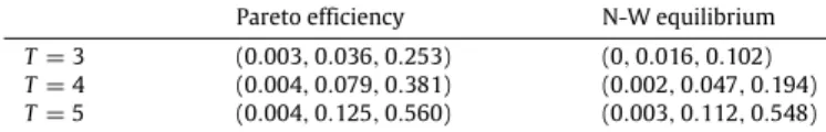
Pareto efficiency N-W equilibrium T=3 (0.003,0.036,0.253) (0,0.016,0.102) T=4 (0.004,0.079,0.381) (0.002,0.047,0.194) T=5 (0.004,0.125,0.560) (0.003,0.112,0.548)

commodities: in each cell, the first number is for the test without warm-glow effects, the second number is for the test with them. As the table shows, the MIP method can accommodate multiple observations, agents and commodities, and the test can be imple-mented in reasonable time.

Without public goods, the test of Walras equilibrium has been

implemented by Cherchye et al. (2011b).10 _{Although the data}

passes their test, they also observe that the power of that test is

null.11 _{They show, however, that if individual consumption can}

be (at least partially) observed, then the power can be reasonably high. The scenario they consider is that the lower bound of

individ-ual consumption is known, i.e., xi_t ⩾

κ ˆ

xi_t, where

κ ∈ [

0

,

1

]

, andx

ˆ

i_t

is the true consumption level.

In the following, we compare the power of our two MIP tests, without warm-glow effects, using Monte Carlo simulations based

on the procedure inBronars(1987). We draw price data from the

uniform distribution U

[

50

,

100

]

, and individual income data from

U

[

10000

,

11000

]

, to generate high price variation and low income

variation. Then, we randomly choose a share si

t from U

[

0

,

1

]

and

construct ‘‘artificial’’ variables

ˆ

xi_t

=

s i tmit pt and y

ˆ

i_t

=

(1

−

s i t)mit qt

.

Finally, we construct the aggregate endowments Et

=

∑

i

ˆ

xitand

Kt

=

∑

iy

ˆ

it, guaranteeing consistency between nominal and real

variables in the simulations.

The MIP tests are implemented one thousand times for each

hypothesis. The pure test ofPropositions 1and3implies that there

is absolutely no information on the individual consumption of

commodities, in the spirit ofBrown and Matzkin(1996). Following

the ideas ofCherchye et al.(2011b), we then run the tests again,

imposing the constraints that xi

t ⩾

κ ˆ

xit, considering two cases:

‘‘partial observation’’, where

κ =

0

.

9; and ‘‘full observation’’,

where

κ =

1. As inBronars(1987), the alternative hypothesis is

that individuals exhaust their budgets randomly.

Table 2records the power of the tests: in each cell, the first number is the power when there is no information on individ-ual private consumption, the second number is the power under partial observation, and the third number is the power under full observation. As in the case of pure competitive equilibrium first 10_{They assume that all agents within the same US region are the same type of} tastes and incomes, and use regional data from the US economy (8 regions, 12 annual observations, and 18 commodities) to implement their test.

11_{Cherchye et al.}₍_2011b_{) attribute the low test power to low price variation and} high income increase across observations, and conjecture that their test ‘‘may ef-fectively have reasonable power if the data show sufficient price variation together with low income variation’’.

(8)

proposed byBrown and Matzkin(1996), the power of our tests

is very low when no information of individual consumption is known. However, knowing some lower bounds for individual con-sumption will significantly increase the power, especially when

the number of observations is large.12

Note that even the full observation of individual consumption does not make our tests vacuous. Without public goods as in

Cherchye et al.(2011b), GARP or Afriat inequalities can be checked efficiently when individual consumption can be fully observed, and the MIP method does not have any advantage. Nevertheless, when there are public goods (with or without warm-glow effects), the personalized prices cannot be observed and the difficulty of nonlinearity does not disappear. In this case, our tests are easy to implement and our simulation exercises suggest that they are suitable for examining efficiency and competition in economies with public goods. We see our tests as complementary to other methods used in applied work.

Appendix A. Lemmata

Lemma 1 (Cherchye et al., 2011b). Consider a finite set

{

(

π

t

, χ

t)

:

t

=

1

, . . . ,

T

} ⊆

Rλ+

×

Rλ+

.

13 The following statements

are equivalent:

1. The set satisfies GARP: for any finite sequence (tn)Nn=1of indices

in

{

1

, . . . ,

T

}

,

(

π

tn

· χ

tn+1 ⩽

π

tn

· χ

tn

, ∀

n

=

1

, . . . ,

N

−

1)

⇒

π

_t_N

· χ

_t₁ ⩾

π

tN

· χ

tN

.

2. There exists a solution,

{

υ

t,s

∈ {

0

,

1

} |

t

,

s

=

1

, . . . ,

T

;

t

̸=

s

}

, to Cherchye et al.’s Integer Consumer System, CS.I: letting

β =

maxt

{

π

t

· χ

t

} +

1,

(a) for each pair of distinct observations,

π

t

· χ

t

−

π

t

· χ

s

< υ

t,s

· β

and

π

t

· χ

t

−

π

t

· χ

s⩽(1

−

υ

s,t)

· β;

(b) for each triple of distinct observations,

υ

t,s

+

υ

s,r ⩽1

+

υ

t,r

.

Proof. SeeCherchye et al.(2011b). □

Lemma 2. Consider a finite set

{

(pt

,

qt

,

xt

,

yt

, ¯

yt

,

mt)

∈

RL+

×

R+

×

RL+

×

_R+

×

_R+

×

_R+

:

t

=

1

, . . . ,

T

}

.

The following statements are equivalent:

1. The set satisfies the Forges–Minelli generalized version of GARP:

for any finite sequence (tn)Nn=1of indices in

{

1

, . . . ,

T

}

,14

[

gtn(xtn+1

,

ytn+1

+ ¯

ytn+1)⩽0

, ∀

n

=

1

, . . . ,

N

−

1

]

⇒

gtN(xt1

,

yt1

+ ¯

yt1)⩾0

,

(9) where15 gt(x

,

y)

=

max

{

pt

·

x

+

qt

·

y

−

mt

−

qt

· ¯

yt

,

pt

·

x

−

mt

} ;

(10)

12_{In the simulation of both tests with warm-glow effects, not reported here, we} get similar results: the power is low without information on individual private consumption, and reasonably high when (partially) observing individual private consumption.

13_{For the purpose of this lemma, the reader may assimilate}_π

t =(pt,qt),χt = (xt,yt) andλ =L+1.

14_{The following equation re-expresses Eq.}₍₄₎_{in general notation.} 15_{Consistently, the following is a re-expression of Eq.}₍₃₎_.

2. There exists a solution,

{

ω

t,s

∈ {

0

,

1

} |

t

,

s

=

1

, . . . ,

T

;

t

̸=

s

}

,

to the following generalization of Cherchye et al.’s Integer Con-sumer System, CS.I: letting

c

=

max

t

{

pt

·

xt

+

qt

·

(yt

+ ¯

yt)

} +

1

,

(a) for each pair of distinct observations,

pt

·

(xt

−

xs)

+

qt

·

[(yt

+ ¯

yt)

−

max

{

ys

+ ¯

ys

, ¯

yt

}

]

< ω

t,s

·

c

and

pt

·

(xt

−

xs)

+

qt

·

[(yt

+ ¯

yt)

−

max

{

ys

+ ¯

ys

, ¯

yt

}

]

⩽(1

−

ω

_s_,_t)

·

c

;

(b) for each triple of distinct observations,

ω

t,s

+

ω

s,r ⩽1

+

ω

t,r.

Proof. We first argue that statement 1 implies statement 2, by constructing a solution to the system introduced in the latter. Say

that

ω

t,s

=

1 if there exists a finite sequence (tn)Nn=1such that

t1

=

t, tN

=

s and gtn(xtn+1

,

ytn+1

+ ¯

ytn+1) ⩽ 0

.

Otherwise, let

ω

t,s

=

0.

First, suppose that gt(xs

,

ys

+ ¯

ys) ⩽ 0. Then,

ω

t,s

=

1 and,

therefore,

ω

t,s

·

c⩾pt

·

xt

+

qt

·

(yt

+ ¯

yt)

⩾pt

·

xt

+

qt

·

(yt

+ ¯

yt)

−

pt

·

xs

−

qt

·

max

{

ys

+ ¯

ys

, ¯

yt

}

.

If, on the other hand, gt(xs

,

ys

+ ¯

ys)

>

0, then

0

<

max

{

pt

·

xs

+

qt

·

(ys

+ ¯

ys)

−

mt

−

qt

· ¯

yt

,

pt

·

xs

−

mt

}

=

pt

·

xs

−

mt

+

qt

·

max

{

ys

+ ¯

ys

− ¯

yt

,

0

}

=

pt

·

xs

−

(pt

·

xt

+

qt

·

yt)

+

qt

·

max

{

ys

+ ¯

ys

− ¯

yt

,

0

}

=

pt

·

(xs

−

xt)

+

qt

·

[max

{

ys

+ ¯

ys

− ¯

yt

,

0

} −

yt]

=

pt

·

(xs

−

xt)

+

qt

·

[max

{

ys

+ ¯

ys

, ¯

yt

} −

(yt

+ ¯

yt)]

.

Together, these two inequalities imply that, in any case,

pt

·

(xt

−

xs)

+

qt

·

[(yt

+ ¯

yt)

−

max

{

ys

+ ¯

ys

, ¯

yt

}

]

< ω

t,s

·

c

.

(

∗

)

Now, suppose that

ω

s,t

=

1. By construction, there is a sequence

(tn)Nn=1for which t1

=

s, tN

=

t and gtn(xtn+1

,

ytn+1

+ ¯

ytn+1)⩽0

.

By

our generalization of GARP, Eq.(9), then gt(xs

,

ys

+ ¯

ys)⩾0

,

which

implies, right away, that

pt

·

(xt

−

xs)

+

qt

·

[(yt

+ ¯

yt)

−

max

{

ys

+ ¯

ys

, ¯

yt

}

]

⩽(1

−

ω

_s_,_t)

·

c

.

(

∗∗

)

If, on the other hand,

ω

s,t

=

0, the latter is immediate, by

construc-tion.

Eqs.(

∗

)and(

∗∗

)together imply condition (a) of statement 2.

For condition (b), we show that if

ω

t,s

=

ω

s,r

=

1, then

ω

t,r

=

1.

For this, there exist finite sequences (tn)N_n=1and (sm)

M

m=1, such that

t1

=

t, tN

=

s, s1

=

s, sM

=

r,

gtn(xtn+1

,

ytn+1

+ ¯

ytn+1)⩽0 and gsm(xsm+1

,

ysm+1

+ ¯

ysm+1)⩽0

.

Concatenating these sequences as (rl)N

+M

l=1

=

(t1

,

ts

, . . . ,

tN

,

s1

,

ss

,

. . . ,

sM)

,

we get that

ω

t,r

=

1, by definition.

To show that statement 2 implies statement 1, let (

ω

t,s)t̸=s

satisfy conditions (a) and (b) in statement 1, and let finite sequence

(tn)Nn=1be such that for all n

=

1

, . . . ,

N

−

1

,

gtn(xtn+1

,

ytn+1

+

¯

ytn+1)⩽0. Then, for each n⩽N

−

1,

max

{

ptn

·

xtn+1

+

qtn

·

(ytn+1

+ ¯

ytn+1)

−

mtn

−

qtn

· ¯

ytn

,

ptn

·

xtn+1

−

mtn

}

⩽0

.