www.mech-sci.net/4/153/2013/ doi:10.5194/ms-4-153-2013
©Author(s) 2013. CC Attribution 3.0 License.
Mechanical
Sciences
Open AccessMultiple-task motion planning of non-holonomic
systems with dynamics
A. Ratajczak and K. Tcho ´n
Institute of Computer Engineering, Control and Robotics, Wrocław University of Technology, ul. Janiszewskiego 11/17, 50–372 Wrocław, Poland
Correspondence to:A. Ratajczak (adam.ratajczak@pwr.wroc.pl)
Received: 14 November 2012 – Revised: 15 March 2013 – Accepted: 5 April 2013 – Published: 15 April 2013
Abstract. This paper addresses the motion planning problem in non-holonomic robotic systems. The system’s kinematics and dynamics are represented as a control affine system with outputs. The problem is defined in terms of the end-point map of this system, using the endogenous configuration space approach. Special attention is paid to the multiple-task motion planning problem, i.e. a problem that beyond the proper motion planning task includes a number of additional tasks. For multiple-task motion planning two strategies have been proposed, called the egalitarian approach and the prioritarian approach. Also, two computational strategies have been launched of solving the motion planning problem: the parametric and the non-parametric. The motion planning and computational strategies have been applied to a motion planning problem of the trident snake robot. Performance of the motion planning algorithms is illustrated with computer simulations.
1 Introduction
The motion planning problem of a robotic system consists in determining an action in the configuration space that would drive the system along a desired trajectory or to a desired location in the task space. Frequently, reaching the goal is accompanied with avoiding obstacles and singularities, re-specting constraints of motion, limitations of energy, etc. If the planning problem is decomposed into a number of tasks, it is called a multiple-task problem. Resolving multiple-task motion planning problems is enabled by the system’s redun-dancy.
In the area of kinematic control of redundant manipula-tion robots the multiple-task problems have been addressed within the prioritized approach, initiated by Maciejewski and Klein (1985); Nakamura et al. (1987), and then refined in the works of Chiaverini (1997); Chiacchio et al. (1991); Choi et al. (2004); Antonelli (2009). An extension of these ideas towards mobile robotic systems, in particular mobile robots and mobile manipulators, has been promoted by the endogenous configuration space approach (Tcho´n and Jaku-biak, 2003; Tcho´n and Zadarnowska, 2003). The endogenous configuration space approach employs a control system
rep-resentation of the robotic system and focuses on the analy-sis of its end-point map. The central concept of endogenous configuration is identified with the system’s control function, so singular controls become singular endogenous configura-tions, and controllability defines the dexterity of the robotic system. The concept of Jacobian of the robotic system relies on the linear approximation of the control system. Jacobian algorithms are introduced using the continuation method. On the kinematics level the endogenous configuration ap-proach has been developed on the basis of the ideas of Suss-mann (1993); Chitour and SussSuss-mann (1998); Divelbiss et al. (1998). Founded on the end-point map of a control system, the endogenous configuration space approach extends in a natural way to robotic systems with dynamics (Zadarnowska and Tcho´n, 2007; Ratajczak et al., 2010). Since the endoge-nous configuration space is infinite-dimensional, the mobile robotic systems have infinite redundancy, capable of accom-modating an arbitrary big number of tasks. Using the endoge-nous configuration space approach, a prioritized approach to motion planning of underactuated robotic systems has been proposed in Ratajczak et al. (2010); Ratajczak (2012).
models of non-holonomic robotic systems. It is assumed that the proper motion planning task of reaching a desired point in the task space has been supplemented by a number of ad-ditional tasks, characterized by their specific task maps. Two methods of solving the problem have been proposed, called the egalitarian and the prioritarian approach. A motion plan-ning algorithm has been derived by means of the endogenous configuration space approach, in the form of a functional dif-ferential equation for the control function. Furthermore, a parametric and a non-parametric strategy of computing nu-merically the control function have been launched.
Theoretical concepts are applied to the dynamics model of the trident snake robot (Ishikawa, 2004). The robot can be regarded as a realization of the undulatory locomotion princi-ple and a demanding test bed of motion planning algorithms for non-holonomic systems. The design and kinematics anal-ysis of the trident snake with passive wheels and active joints can be found in Ishikawa (2004); Ishikawa et al. (2010). Re-cently, this analysis has been extended to the case of active wheels in Paszuk et al. (2012) and complemented by a study of trident snake dynamics (Pietrowska, 2012). In both these cases the motion single-task planning algorithms have been derived from the endogenous configuration space approach.
Differently than in the references mentioned above, this paper concentrates on the multiple-task motion planning strategy for the trident snake robot. The robot’s kinemat-ics and dynamkinemat-ics are represented as a control affine sys-tem with outputs. The problem is defined in terms of the end-point map of this system. The control strategy of the system involves a preliminary state feedback. The motion planning problem includes two subtasks: the proper mo-tion planning task of transferring the system to a desired task space location, and the singularity avoidance task guar-anteeing well definiteness of the feedback transformation. Two motion planning strategies have been developed, re-ferred to as the egalitarian and the prioritarian approach. The former strategy regards the component tasks as equivalent, the latter assigns the highest priority to the proper motion planning task. Simultaneously, two computational strategies have been proposed in order to solve the motion planning problem: the parametric and the non-parametric, depending on whether the computation of the control function utilizes a specific base in the endogenous configuration space or is base-independent. Computer simulations demonstrate the performance of the egalitarian non-parametric and the prior-itarian parametric motion planning algorithms.
The paper is organized in the following way. Section 2 introduces a control system representation of the non-holonomic system, defines a Jacobian motion planning al-gorithm, and describes two computational strategies. The strategies of multiple-task motion planning are presented in Sect. 3. In Sect. 4 the motion planning strategies are specified to the trident snake robot. Results of numeric computations are included in Sect. 5. Section 6 concludes the paper. In or-der to not distract the reaor-der’s attention from the main thread
of the paper, a derivation of the subtask Jacobian and its in-verse as well as the dynamics model of the trident snake are placed in the Appendix.
2 Basic concepts
Since the dynamics of a non-holonomic robotic system can be represented as an affine control system with outputs, this system will define ouruniverse of discourse. We begin with introducing basic concepts of the endogenous configuration space approach, and derive the Jacobian motion planning al-gorithm. This algorithm relies on the solution of a functional differential equation involving a Jacobian inverse operator. Depending on the method of solution of this equation, para-metric or non-parapara-metric motion planning algorithms are dis-tinguished.
2.1 Endogenous configuration space approach
The basic concepts of the endogenous configuration space approach will be adopted to a general control affine system, of the form
( x˙=f(x)+g(x)u= f(x)+Pm
i=1gi(x)ui,
y=k(x), (1)
whereu∈Rm, x∈Rn, y∈Rr. All the functions and vector
fields appearing in (1) will be assumed smooth. Let T>0 denote a control time horizon. The admissible control func-tions entering system (1) will be assumed to belong to the space L2
m[0,T] of Lebesgue square integrable functions de-fined on the interval [0,T]. The space L2
m[0,T] is a Hilbert space with inner product
hu1(·),u2(·)iR= T
Z
0
uT1(t)R(t)u2(t)dt, (2)
where R(t)=RT(t)>0, and the corresponding norm ||u(·)||R=hu(·),u(·)i1R/2. For a control function u(·), let x(t)=ϕx0,t(u(·)) denote the state trajectory of (1), initialized atx0. It will be assumed that this trajectory exists for every
t∈[0,T]. The outputyis identified with the vector of task variables.
Given an initial statex0of system (1) and the time horizon
T, a general motion planning problem consists in defining a controlu(t) that drives the system’s output atT to a pre-scribed pointyd, so thaty(T)=yd.
Our analysis of the motion planning problem will be based on the concept of the end-point map of system (1), defined as the value atT of the output function resulting from the application of a control functionu(·),
(Sontag, 1990). In the context of mobile robots or mobile ma-nipulators the spaceXhas been called the endogenous con-figurations space (Tcho´n and Jakubiak, 2003). The derivative of the end-point map is computed by means of the linear ap-proximation to system (1)
˙
ξ(t)=A(t)ξ(t)+B(t)v(t), η(t)=C(t)ξ(t), ξ(0)=0, (4)
along the (control,trajectory) pair (u(t),x(t)), where
ξ(t)=Dϕx0,t(u(·))v(·), (5)
and
A(t) = ∂(f(x(t))+g(x(t))u(t))
∂x , B(t)=g(x(t)),
C(t) = ∂k(x(t))
∂x . (6)
Given the linear system (4), the derivative of the end-point map atu(·)∈ Xis equal to
DKx0,T(u(·))v(·)=η(T)=C(T)ξ(T). (7) In compliance with the robotic terminology, the derivative (7) will be called the system’s Jacobian,
DKx0,T(u(·))v(·)=Jx0,T(u(·))v(·).
It follows that the computation of the Jacobian involves the integration of the differential equation (4) from 0 toTat zero initial condition. IfΦ(t,s) denotes the transition matrix of (4),
∂Φ(t,s)
∂t =A(t)Φ(t,s), Φ(s,s)=In,
this means that the JacobianJx0,T(u(·)) :X −→R r
can be ex-pressed as
Jx0,T(u(·))v(·)=C(T) T
Z
0
Φ(T,s)B(s)v(s)ds. (8)
The Jacobian allows to distinguish regular and singular con-trols (endogenous configurations) of system (1). A control u(·)∈ X will be called regular, if the Jacobian is surjective ontoRr, otherwise the controlu(·) is referred to as singular. It can be shown that at regular controls the control affine sys-tem (1) is locally controllable.
Using the inner product (2) in the endogenous configura-tion space and the Euclidean structure of the output space, the dual Jacobian mapJ∗x0,T(u(·)) :Rr−→ X can be defined
in the following way
J∗x0,T(u(·))η
(t)=R−1(t)BT(t)ΦT(T,t)CT(T)η. (9)
2.2 Jacobian motion planning
Using the end-point map, the general motion planning prob-lem in system (1) is tantamount to computing a control functionud(·), such that Kx0,T(ud(·))=yd. The problem can be solved by means of a Jacobian motion planning algo-rithm whose derivation relies on the continuation (homotopy) method (Sussmann, 1993). Given the motion planning prob-lem, we begin with any initial control u0(·)∈ X. If the
ini-tial choice does not solve the problem, i.e.Kx0,T(u0(·)),yd, we choose inXa differentiable curveuθ(·),θ∈R, passing at
θ=0 throughu0(·), and compute the task space error along
this curve
e(θ)=Kx0,T(uθ(·))−yd. (10)
Next, we request that the error decrease exponentially along withθ, with a prescribed decay rateγ >0, i.e.
de(θ)
dθ =−γe(θ). (11)
By differentiating the formula (10) with respect toθ, we ar-rive at the Wa˙zewski-Davidenko equation
Jx0,T(uθ(·)) duθ(·)
dθ =−γe(θ), (12)
involving the Jacobian (8). If J#x0,T(u(·)) :Rr−→ X denotes
a right Jacobian inverse, such that Jx0,T(u(·))J
#
x0,T(u(·))=Ir, then (12) can be converted into a dynamic system
duθ(·)
dθ =−γJ
#
x0,T(uθ(·))e(θ) (13)
evolving in X. Finally, a solution of the motion planning problem is obtained as the limit
ud(t)= lim
θ→+∞uθ(t).
A frequently used right Jacobian inverse is the Moore– Penrose inverse derived from minimizing the square norm ||v(·)||2Runder the equality constraint (a Jacobian equation)
Jx0,T(u(·))v(·)=η, (14)
η∈Rr. The resulting formula is (Tcho´n and Jakubiak, 2003),
J#x0,T(u(·))η
(t)=R−1(t)BT(t)ΦT(T,t)CT(T)G−1x0,T(u(·))η, (15) where
Gx0,T(u(·))=C(T) T
Z
0
Φ(T,s)B(s)R−1(s)BT(s)ΦT(T,s)dsCT(T).
or mobility matrix of system (1) (Tcho´n and Zadarnowska, 2003). At regular control functions the Gram matrix is full rank, making the inverse (15) well defined. The Gram matrix can be conveniently computed by integrating the Lyapunov differential equation
˙
M(t)=B(t)R−1(t)BT(t)+A(t)M(t)+M(t)AT(t), (16)
at zero initial condition M(0)=0, and then substituting Gx0,T(u(·))=C(T)M(T)CT(T). By invoking the definition of
dual Jacobian (9), it is easily checked that the Gram matrix equals the composition
Gx0,T(u(·))=Jx0,T(u(·))J
∗
x0,T(u(·)).
Moreover, it follows that the Jacobian inverse (15) can be written as
J#x0,T(u(·))η
(t)=J∗x0,T(u(·))G
−1
x0,T(u(·))η
(t),
what justifies the identity
J#x0,T(u(·))=J
∗
x0,T(u(·))G
−1
x0,T(u(·)). (17)
2.3 Computations
The Jacobian motion planning algorithm derived in the previ-ous subsection exploits a solution of a functional differential equation (13) in the endogenous configuration spaceX. In order to make this equation tractable, we need to discretize theθvariable, and pass to a discrete control updating scheme
uθ+1(t)=
uθ(t)−γR−1(t)BTθ(t)Φ
T
θ(T,t)C
T
θ(T)G
−1
x0,T(uθ(·))e(θ), (18) whereBθ(t),Φθ(t,s),Cθ(t) are computed along (uθ(t),xθ(t))
in agreement with (6), and e(θ)=Kx0,T(uθ(·))−yd, for θ= 0,1, . . ..
Givenuθ(t), a basic step of the updating (18) consists in
solving simultaneously a system of differential equations
˙
xθ(t)=f(xθ(t))+g(xθ(t))uθ(t), ∂Φθ(T,t)
∂t =−Φθ(T,t)Aθ(t), ˙
Mθ(t)=Bθ(t)R−1(t)BTθ(t)+Aθ(t)Mθ(t)+Mθ(t)ATθ(t)
with respective boundary conditions xθ(0)=x0,Φθ(T,T)=
InandMθ(0)=0.
Alternatively, we can expand the control functions into a truncated orthogonal series that leads to a finite parametriza-tion of controls. More specifically, we select a finite base of orthogonal functions{ϕ0(t), ϕ1(t), . . . , ϕk(t)}, and assume that
uλ(t)= Ψ(t)λ, uλi(t)=
k
X
j=0
ϕj(t)λi j, i=1,2, . . . ,m,
whereλ∈Rs,s=m(k+1), and matrixΨ(t) of dimensionm×s contains the suitably arranged basic functions. By orthogo-nality of the baseR0TΨT(t)Ψ(t)dt=Is. Under assumption that v(t)= Ψ(t)µ, the Jacobian (8) takes the matrix form
ˆ
Jx0,T(λ)=Cλ(T)
T
Z
0
Φλ(T,s)Bλ(s)Ψ(s)ds,
where the matrices (6) need to be computed foru(t)=uλ(t)
andx(t)=ϕx0,t(uλ(·)). It follows that this Jacobian can be ob-tained by the integration of the matrix differential equation
˙
Nλ(t)=Bλ(t)Ψ(t)+Aλ(t)Nλ(t)
with initial condition Nλ(0)=0, followed by the
substitu-tion ˆJx0,T(λ)=Cλ(T)Nλ(T). For the matrix Jacobian, the Ja-cobian equation (14) assumes the form ˆJx0,T(λ)µ=η. It can be shown that the Moore–Penrose Jacobian inverse assumes the matrix form
ˆ
J#x0,T(λ)=S
−1ˆ
Jx0,T(λ)
ˆ Jx0,T(λ)S
−1ˆ
JTx0,T(λ)
−1
, (19)
where S =RT 0 Ψ
T(t)R(t)Ψ(t)dt. Consequently, the updating
scheme of the control function (18) converts to
λθ+1=λθ−γJˆ#x0,T(λθ)e(θ). (20)
The representation of the control functions by means of a truncated orthogonal series will be called parametric. By contrast, the representation that does not use any base will be referred to as non-parametric. This terminology extends to the corresponding motion planning algorithms.
3 Multiple-task motion planning
If the motion planning problem consists only of the motion planning task, it will be called single-task. When the motion planning task is augmented with additional tasks, the motion planning problem will be referred to as a multiple-task prob-lem. We shall assume that the additional tasks are defined by task mapsiK
x0,T:X −→R i=1,2, . . . ,p, operating in the en-dogenous configuration space of (1). Most frequently, these task maps have the form
i
Kx0,T(u(·))= T
Z
0
Fi(x(t),u(t))dt, (21)
for a non-negative functionFi(x,u)≥0 that is assumed dif-ferentiable wherever defined. Given p additional tasks, the multiple-task motion planning problem consists in determin-ing a control functionu(·)∈ Xminimizing the collective error
where 0e(θ)=K
x0,T(uθ(·))−yd and ie(θ)=iKx0,T(uθ(·)) i=
1,2, . . . ,p are errors corresponding to subsequent subtasks. We associate with the task maps the Jacobians: the Jacobian for the task number 0 is given by (8), while for thei-th sub-task the Jacobian
i
Jx0,T(u(·))v(·)= T
Z
0
∂Fi(x(t),u(t))
∂x ξ(t)+
∂Fi(x(t),u(t))
∂u v(t)
!
dt, (23)
whereξ(t) denotes the solution of (4), see Appendix for a derivation. The Moore–Penrose inverse for0J
x0,T(u(·)) is de-fined by expression (15). In Appendix we have shown that the Moore–Penrose inverse of theith Jacobian,i=1,2, . . . ,p, takes the following form
i
J#x0,T(u(·))η
(t)= bi(t)+ci(t) ||bi(·)+ci(·)||2
R
η, (24)
η∈R, where
bi(t)=R−1(t)BT(t) T
Z
t
ΦT(s,t) ∂Fi(x(s),u(s))
∂x
!T
ds, (25)
ci(t)=R−1(t) ∂Fi(x(t),u(t))
∂u
!T
. (26)
The task Jacobians can be arranged into a collective Jacobian
Jx0,T(uθ(·))v(·)=
0
Jx0,T(u(·))v(·),
1
Jx0,T(u(·))v(·), . . . , p
Jx0,T(u(·))v(·)
. (27)
These subtasks can either be treated as equivalent and solved simultaneously or ordered according to their importance and solved sequentially. These two approaches will be further re-ferred to as egalitarian and prioritarian. In the following two subsections we shall derive an egalitarian and a prioritarian Jacobian motion planning algorithm.
3.1 Egalitarian approach
In accordance with the egalitarian approach all subtasks need to be solved simultaneously. Imposing the exponential de-crease of the error (22) with a decay rate γ >0, and us-ing the collective Jacobian (27), we arrive at the Wa˙zewski-Davidenko equation
Jx0,T(uθ(·)) duθ(·)
dθ =−γe(θ). (28)
Finally, similarly to (13), the equation (28) can be solved by means of the Moore–Penrose Jacobian inverse of the collec-tive Jacobian,
duθ(·)
dθ =−γJ
#
x0,T(uθ(·))e(θ). (29)
The egalitarian solution of the multiple-task motion planning problem is obtained as the limitud=limθ→+∞uθ(t) of the
tra-jectory of dynamic system (29).
3.2 Prioritarian approach
Differently to the egalitarian algorithm, now the subtasks will be ordered with decreasing priorities. The essential assump-tion of the prioritarian approach is that the soluassump-tion of a lower priority task is sought in a space rendered accessible by the higher priority tasks, so it should not affect the solution of any task with higher priority. Given thei-th error (22) and thei-th Jacobian (27), we start the derivation from a state-ment of the Jacobian equation for thei-th subtask,
die(θ)
dθ =
i
Jx0,T(uθ(·)) duθ(·)
dθ =−
iγi
e(θ), (30)
withiγ >0 andi=0,1, . . . ,p. A general solution of this equa-tion involves the Jacobian inverse with projecequa-tion (Tcho´n and Jakubiak, 2003),
duθ(·)
dθ =−
iγi
J#x0,T(uθ(·)) i
e(θ)+iPx0,T(uθ(·)) iζ
θ(·), (31)
where
i
Px0,T(uθ(·))=idX− i
J#x0,T(uθ(·))iJx0,T(uθ(·)) denotes the projection onto keriJx0,T(uθ(·)), and
iζ
θ(·)∈ Xis
any element of the endogenous configuration space. For the highest priority task (number 0) the equality (31) is required to hold in the whole endogenous configuration space,
duθ(·)
dθ =−
0γ0
J#x0,T(uθ(·))
0
e(θ)+0Px0,T(uθ(·))
0ζ
θ(·). (32)
For the lower priority task (number 1) this equality needs to be satisfied only within the kernel of0J#
x0,T(uθ(·)), i.e.
0
Px0,T(uθ(·)) duθ(·)
dθ =−
1γ0
Px0,T(uθ(·))
1
J#x0,T(uθ(·))1e(θ)
+0Px0,T(uθ(·))
1
Px0,T(uθ(·))
1ζ
θ(·). (33)
Having projected (32) onto ker0Jx0,T(uθ(·)), we get
0
Px0,T(uθ(·))
duθ(·)
dθ =
0
Px0,T(uθ(·))0ζθ(·), (34)
where we have used the identityiPx0,T(uθ(·)) i
J#x0,T(uθ(·))=0, and the idempotency of the projection. Now, a combination of (33) and (34) results in
0
Px0,T(uθ(·))
0ζ
θ(·)=−1γ0Px0,T(uθ(·))
1
J#x0,T(uθ(·))
1
e(θ)
+0Px0,T(uθ(·))1Px0,T(uθ(·))1ζθ(·).
Finally, a substitution of the above identity into (32) yields the following prioritarian Jacobian motion planning algo-rithm for two subtasks
duθ(·)
dθ =−
0γ0
J#x0,T(uθ(·))
0
e(θ)−1γ0Px0,T(uθ(·))
1
J#x0,T(uθ(·))
1
e(θ)
+0Px0,T(uθ(·))
1
Px0,T(uθ(·))
1ζ
If there are only two subtasks, the last term1ζ
θ(·) is zero,
otherwise it could be used to define the prioritarian algorithm for the remaining lower priority tasks.
In this way the presented derivation extends top+1 sub-tasks, resulting in the following motion planning algorithm (Ratajczak et al., 2010; Ratajczak, 2012),
duθ(t)
dθ =−
p X i=0 iγ i Y j=0 j−1
Px0,T(uθ(·))
i
J#x0,T(uθ(·)) i
e(θ), (36)
where−1P
x0,T(uθ(·))=idX. In the terminology of Antonelli (2009) this algorithm belongs to the successive inverse-based projection methods. Again, the solution of the multiple-task motion planning problem is obtained as the limit ud(t)=
limθ→+∞uθ(t) of the trajectory of system (36).
Let us take a closer examination of the control formula (35). By a substitution of this formula into (32), it is easily seen that the first error
d0e(θ)
dθ =−
0γ0
e(θ)
decreases exponentially, as requested in (11). However, be-cause of the task-priority assumption, the second error
d1e(θ) dθ =−
1γ1
e(θ)−0γ1Jx0,T(uθ(·))
0
J#x0,T(uθ(·))
0
e(θ)
+1γ1Jx0,T(uθ(·))0J
#
x0,T(uθ(·))
0
Jx0,T(uθ(·))1J
#
x0,T(uθ(·))
1
e(θ),
behaves differently. The error1e(θ) will converge toward zero
exponentially, provided that it does not affect convergence of the error0e(θ). This happens when1J
x0,T(uθ(·))
0J#
x0,T(uθ(·))= 0. Taking into account the form of (17), the last equality will be satisfied whenever
1
Jx0,T(uθ(·))
0
J∗x0,T(uθ(·))=0,
what may be interpreted as a sort of orthogonality of Jaco-bians0Jx0,T(u(·)) and
1
Jx0,T(u(·)).
4 Motion planning of trident snake
The presented algorithms will be utilized in order to solve a motion planning problem for the trident snake mobile robot (Ishikawa, 2004; Ishikawa et al., 2010; Paszuk et al., 2012). In the following subsections we are going to present a control-theoretic model, state a multiple-task motion plan-ning problem, and introduce the egalitarian and the prioritar-ian motion planning algorithm for the trident snake robot.
4.1 Model
The trident snake is a non-holonomic mobile robot. It con-sists of a triangular-shape body and three links able to rotate around the attachment points (see Fig. 1). Each link is ended with a passive wheel which is subjected to non-holonomic
φ1 φ2 φ3 α1 α3 r l X Y x y θ
Figure 1.Trident snake robot: conceptual model.
constraints. The control inputs of the robot are the driving torques exerted at the joints between the body and the links. The anglesα1=−23π,α2=0,α3=23πare constant
geomet-ric parameters of the robot,ldenotes the length of each link, andrstands for the distance between the center of the robot body and the joints.
4.1.1 Kinematics
According to Fig. 1, the vector of generalized coordinates is defined asq=(x,y, θ, φ1, φ2, φ3)=(x,y, θ, φ)∈R6. For every
wheel the non-holonomic constraints arise from the assump-tion of non-slipping laterally. The corresponding constraints matrix takes the form (Ishikawa et al., 2010; Paszuk et al., 2012)
A(q)=h A1(q)RotT(Z, θ) −lI3 i
,
where Rot(Z, θ) is the rotation matrix around Z-axis byθ an-gle, andA1(q) is defined as
A1(q)=
sin(α1+φ1) −cos(α1+φ1) −l−rcosφ1
sin(α2+φ2) −cos(α2+φ2) −l−rcosφ2
sin(α3+φ3) −cos(α3+φ3) −l−rcosφ3 .
Using the relationA(q)G(q)=0, we find
G(q)=
cosθ −sinθ 0
sinθ cosθ 0
0 0 1
sin(α1+φ1)
l −
cos(α1+φ1)
l −1−
rcosφ1 l
sin(α2+φ2)
l −
cos(α2+φ2)
l −1−
rcosφ2 l
sin(α3+φ3)
l −
cos(α3+φ3)
l −1−
rcosφ3 l = "
G1(θ)
G2(φ) #
so the trident snake kinematics can be represented by the driftless control system
˙
q=G(q)v,
v∈R3denoting the control variable.
4.1.2 Dynamics
The dynamics equations of the trident snake can be obtained from the Lagrange formalism together with the d’Alembert principle. A detailed derivation can be found in Pietrowska (2012). After the elimination of the traction forces, the re-sulting equations of motion take the form
˙
q=G(q)v ˙
v=N(q,v)+P(q)w,
y=k(q,v).
(38)
The matrixG(q) is given by (37), the termsN(q,v) andP(q) can be reconstructed from the data provided in the Sect. A2. It follows that the trident snake has dimv=dimw=3, so it is fully controlled. Therefore, it is possible to apply a partially linearizing feedback transformation
w=P−1(q) (u−N(q,v)), (39)
udenoting a new control variable, that simplifies the control system representation substantially, and produces a kinemat-ically reduced system (Lewis, 1999),
˙
q=G(q)v ˙
v=u,
y=k(q,v).
(40)
In Paszuk et al. (2012), it has been shown that the feedback (39) is well defined provided that the lower submatrix of (37) is non-singular, i.e. detG2(φ),0.
To obtain a control affine system (1), we need to introduce a state vector x=(q,v)∈R9. Then, the kinematics and
dy-namics of the trident snake may be rewritten as
(
˙
x=f(x)+g(x)u,
y=k(x), (41)
whereu∈R3and
f(x)= G(q)v
03×1 !
, g(x)= "
03×3
I3 #
.
Assuming that all state variablesxare subject to motion plan-ning, we get the output functiony=k(x)=x.
4.2 Motion planning
The motion planning problem for the trident snake will con-sist in defining a control function u(t) in system (41) that
drives the system from an initial state to a desired termi-nal output, over a prescribed time horizonT>0. In order to make the feedback (39) well defined, the controlu(t) should also prevent matrixG2(φ) from getting singular. Clearly, the
motion planning problem includes two subtasks, of which the former will be called the proper motion planning task (index 0), whereas the latter will be named the singularity avoidance task (index 1). The task map0K
x0,T(u(·)) is just the end-point map of system (41). The singularity avoidance task will be assigned the task map1Kx0,T(u(·)) of the form (21) with func-tionF1(x,u)=det−2(G2(φ)). The collective errore(θ) and the
collective Jacobian Jx0,T(u(·)) can be derived directly from (22) and (27).
4.3 Algorithms
The motion planning problem for the trident snake robot will be solved by means of the multiple-task motion planning al-gorithms introduced in Sect. 3. For the egalitarian motion planning the collective error is defined as
e(θ)=(0e(θ), δ1e(θ)),
where the second component has been multiplied by a scal-ing factorδin order to maintain a dynamic balance of the two subtasks. The egalitarian motion planning algorithm takes the form (29). The solution is the limitud=limθ→+∞uθ(t) of
the trajectory of (29).
In the prioritarian approach, the proper motion planning subtask will be assigned a higher priority, while the singu-larity avoidance subtask will get a lower priority. Having defined two errors: 0e(θ), 1e(θ) and two Jacobian inverses: 0J#
x0,T(u(·)) and
1J#
x0,T(u(·)) given, respectively, by (15) and (24), we can provide the following formula for the priori-tarian motion planning algorithm (36)
duθ(·)
dθ =
−0γ0J#x0,T(uθ(·))0e(θ)−1γ0Px0,T(uθ(·))
1
J#x0,T(uθ(·))1e(θ),
where0P
x0,T(u(·)) denotes the projection into ker
0J
x0,T(u(·)). In the next section the performance of both these algorithms will be illustrated by means of numerical computations.
5 Implementation and computations
Figure 2.Trident snake robot: physical model.
proper motion planning task consists in driving the system (41) from the initial statex0=(0,0,0,0,0,0,0,0,0) to the
de-siredyd=xd=(0.1,0,0,0,0,0,0,0,0), over the time horizon T=1. Taking into account geometric parameters of the tri-dent snaker=l=0.12, this task could be interpreted as an elementary a rest-to-rest move forward. For both these sim-ulations, the motion planning problem is regarded as solved, when the normk0e(θ)kdrops below 10−4, and the
determi-nant det(G2(φ)),0 during the whole motion time. The
ini-tial control functions for both cases are chosen constant, u0=(2,1,−1). In the egalitarian algorithm the error decay
rate γ=0.1, and the scaling factor δ=10−4. The prioritar-ian algorithm uses decay coefficients0γ=0.5 and1γ=10−3. In the parametric representation a truncated Fourier series of lengthk=20 has been chosen, so the vector of control pa-rametersλ∈R63. The dynamics model of the trident snake
robot has been borrowed from Pietrowska (2012). The model corresponds to the trident snake robot designed at our labo-ratory, Gospodarek (2011), displayed in Fig. 2. Its dynamic parameters are the following:
– body massm0=0.52kg,
– wheel massmw=0.03kg,
– wheel radiusrw=0.02m,
– wheel thicknessd=0.001m,
– moment of inertia of the body around its center of mass I0=m0r
2
4 ,
– moment of inertia of the wheel around the center of mass of the robot bodyI0w=mw(
r2 w
4 +
d2
12),
– link massml=0.07kg,
– motor massmm=0.055kg,
– total massmc=m0+3(mw+mm+ml).
0 0.05 0.1
−0.1 −0.05 0 0.05 0.1
x
y
0 0.05 0.1
0 0.05 0.1 0.15
x
y
Figure 3.Motion path inXY plane: egalitarian solution (left) and
prioritarian solution (right).
0 0.2 0.4 0.6 0.8 1
−0.6 −0.4 −0.2 0 0.2 0.4 0.6
t
x
,
y
,
v1
,
v2
x y v1 v2
0 0.2 0.4 0.6 0.8 1
−0.6 −0.4 −0.2 0 0.2 0.4 0.6
t
x
,
y
,
v1
,
v2
x y v1 v2
Figure 4.Position and linear velocity: egalitarian solution (top) and
prioritarian solution (bottom).
0 0.2 0.4 0.6 0.8 1 −6
−4 −2 0 2 4 6
t
θ
,
v3
θ v3
0 0.2 0.4 0.6 0.8 1
−4 −3 −2 −1 0 1 2 3
t
θ
,
v3
θ v3
Figure 5. Orientation and angular velocity: egalitarian solution
(top) and prioritarian solution (bottom).
0 0.2 0.4 0.6 0.8 1
−2 −1 0 1 2
t φ1
,
φ2
,
φ3
φ1 φ2 φ3
0 0.2 0.4 0.6 0.8 1
−1.5 −1 −0.5 0 0.5 1 1.5
t φ1
,
φ2
,
φ3
φ1 φ2 φ3
Figure 6.Joint angles: egalitarian solution (top) and prioritarian
solution (bottom).
0 0.2 0.4 0.6 0.8 1
−10 −5 0 5 10 15 20
t u1
,
u2
,
u3
u1
u2
u3
0 0.2 0.4 0.6 0.8 1
−8 −6 −4 −2 0 2 4
t u1
,
u2
,
u3
u1
u2
u3
Figure 7.Linearized controlu(t), egalitarian solution (top) and
pri-oritarian solution (bottom).
0 0.2 0.4 0.6 0.8 1
−1.5 −1 −0.5 0 0.5 1
t w1
,
w2
,
w3
w1 w2 w3
0 0.2 0.4 0.6 0.8 1
−1.5 −1 −0.5 0 0.5 1 1.5 2
t
w
1
,
w2
,
w3
w1 w2 w3
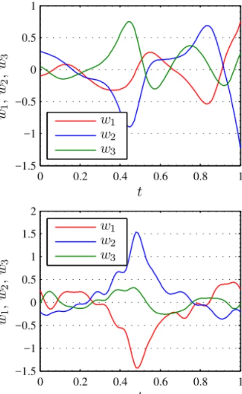
Figure 8.Original controlw(t): egalitarian solution (top) and
0 0.2 0.4 0.6 0.8 1 −4
−3 −2 −1 0
t
d
et
(
G2
(
φ
))
0 0.2 0.4 0.6 0.8 1
−4 −3 −2 −1 0
t
d
et
(
G2
(
φ
))
Figure 9. Determinant det(G2(φ)): egalitarian solution (top) and
prioritarian solution (bottom).
functions obtained from thenon-parametric egalitarian and the parametric prioritarian approaches, one can see that the non-parametric controls are smoother. The original control w(t) representing the torques in the joints is depicted in Fig. 8. Again, as in the case ofu(t) control, the functionw(t) produced by the non-parametric algorithm is smoother. Fig-ure 9 refers to the singularity avoidance subtask. The plots present the value of the determinant det(G2(φ)) during the
motion time. In both algorithms the determinant stays quite far away from zero, what means that the egalitarian and the prioritarian algorithms have solved the second task in a satis-factory way. This conclusion is confirmed by Fig. 10 show-ing three-dimensional plots in the joint space φ. The sur-face det(G2(φ))=0 represents singularities. Joint
trajecto-riesφ(t) (starting with the black color and going towards the light green) remain safely inside the regular set. Finally, the last Fig. 11 illustrates the convergence of the algorithms. It follows that the non-parametric egalitarian algorithm needs more steps in order to fulfill the stop conditionk0e(θ)k<10−4.
In the egalitarian algorithm the total errore(θ) decreases ex-ponentially. In the case of the prioritarian algorithm the error of the second task|1e(θ)|has been forced to increase by the
higher priority task.
Figure 10.Motion in joint spaceφ: egalitarian solution (top) and
prioritarian solution (bottom).
6 Conclusions
0 20 40 60 80 100 120
10−4
10−3
10−2
10−1
100
101
θ
e
(
θ
)
ke(θ)k
k0e
(θ)k
0 10 20 30 40
10−4
10−3
10−2
10−1
100
101
θ
e
(
θ
)
k0e (θ)k
|1e (θ)|
Figure 11.Convergence: egalitarian solution (top) and prioritarian
solution (bottom)top.
algorithms have been applied to solve amultiple-task motion planning problem for the trident snake robot, that consists of the proper motion planning task and the singularity avoid-ance task. Numerical computations have shown that both the algorithms provide correct, although different, solutions to the problem. Also, the algorithms behave differently. In the case of egalitarian algorithm, when all the tasks are solved simultaneously, there are only two possibilities: either both tasks are solved correctly or none of the tasks is solved what-soever. Contrary to that, in the prioritarian algorithm there is a risk that only the highest priority tasks will be solved. This observation has been confirmed by the plots of error convergence. In the egalitarian algorithm the total error de-creases. It follows from the derivation of the prioritarian al-gorithm that the error of a lower priority task can even in-crease to enable the dein-crease of a higher priority task error. The parametric computations of solution of the motion plan-ning problem are base-dependent, what usually appears to be quite restrictive. The non-parametric representation of con-trol functions does not depend on the base choice, and is free from the limitations of the parametric approach. The com-putational effort in the parametric approach depends on the dimension of the parameter space. If the number of parame-ters is small, the parametric computations are much more ef-ficient than the non-parametric. This, however, reverts, when the number of parameters grows up. In the example presented
in this paper (63 control parameters), the parametric compu-tations have been about 1.5 times more time consuming than the non-parametric. This being so, the choice of the motion planning strategy should depend on the complexity of the non-holonomic system subject to motion planning as well as on the type of the tasks defining the problem.
Appendix A
In this section we shall make a derivation of the Jacobian (23) and its Moore–Penrose inverse (24), and present the dynam-ics model of the trident snake robot used in Sect. 4.
A1 Subtask Jacobian and its inverse
Thei-th subtask Jacobian is equal to
i
Jx0,T(u(·))v(·)=D i
Kx0,T(u(·))v(·)
= d
dα
α=0
T
Z
0
Fi(ϕx0,t(u(·)+αv(·)),u(t)+αv(t))dt,
where x(t)=ϕx0,t(u(·)) denotes the state trajectory of (1) driven by the control functionu(·). The differentiation gives
i
Jx0,T(u(·))v(·)
=
T
Z
0
∂Fi(x(t),u(t))
∂x Dϕx0,t(u(·))v(·)+
∂Fi(x(t),u(t))
∂u v(t)
!
dt.
Finally, a substitution for ξ(t)=Dϕx0,t(u(·))v(·) from (5) yields (23).
In order to find a formula for the Moore–Penrose Jacobian inverse, we begin with a Jacobian equation
i
Jx0,T(u(·))v(·)=η,
whereη∈R. A solution of this equation will be sought by
minimizing the squared norm of the control function,
min v(·)
||v(·)||2R=
T
Z
0
vT(t)Rv(t)dt
,
with the equality constraint. After the substitution
ξ(t)=
t
Z
0
Φ(t,s)B(s)v(s)ds,
the corresponding Lagrange function becomes
L(v(·), λ)=
T
Z
0
vT(t)Rv(t)dt+λ
T
Z
0
∂Fi(x(t),u(t))
∂x
t
Z
0
Φ(t,s)B(s)v(s)ds+∂Fi(x(t),u(t))
∂u v(t)dt
λ∈R. Now, the differentiation of the Lagrange function with respect tov(·)
D L(v(·), λ)w(·)= d
dα α=0
L(v(·)+αw(·), λ),
use of the identity
T Z 0 t Z 0
f(t,s)dsdt=
T Z 0 T Z s
f(t,s)dtds,
and then equating the derivative to 0 yield
vi(t)=− 1 2λR
−1
(t)
BT(t) T
Z
t
ΦT(s,t) ∂Fi(x(s),u(s)) ∂x
!T
ds
+ ∂Fi(x(t),u(t))
∂u
!T ,
where the subscripti refers to thei-th subtask. To simplify the notations, let us define a pair of functions
bi(t)=R−1(t)BT(t) T
Z
t
ΦT(s,t) ∂Fi(x(s),u(s))
∂x
!T
ds
and
ci(t)=R−1(t) ∂Fi(x(t),u(t))
∂u
!T
,
so that
vi(t)=−1
2λ(bi(t)+ci(t)).
The Lagrange multiplierλcan be eliminated by inserting the controlvi(t) into the Jacobian equation, that implies
−1 2λ T Z 0
bTi(t)R(t)+c T i(t)R(t)
(bi(t)+ci(t))dt
=−1
2λ||bi(·)+ci(·)||
2
R=η.
From the last identity we computeλ, and conclude that
vi(t)= bi(t)+ci(t) ||bi(·)+ci(·)||2Rη,
what is just (24).
A2 Dynamics model of trident snake
A standard derivation based on the Lagrangian mechanics and d’Alembert principle leads to the following definition of terms appearing in the equations of motion (38) of the trident snake robot
P(q)=M−1
(q)GT (q)B(q),
M(q)=GT(q)Q(q)G(q),
N(q,v)=−M−1(q)GT(q)Q(q) ˙G(q)+C(q,G(q)v)G(q)v,
whereG(q) is given by (37),
B(q)= "
03×3
I3 #
denotes a control matrix,Q(q) is the inertia matrix defined below, andC(q,q˙) is the matrix of Coriolis and centripetal forces whose entries
Ck j(q,q˙)= 6 X
i=1
cki j(q) ˙qi
are determined by the Christoffel’s symbols of the first kind associated withQ(q)
cki j(q)= 1 2
∂Qik(q)
∂qj
+∂Qjk(q)
∂qi
−∂Qi j(q)
∂qk
!
, i,j,k=1, . . . ,6.
The following form of the inertia matrix for the trident snake robot can be found in Pietrowska (2012)
Q(q)=
m11 0 m13 m14 m15 m16
0 m22 m23 m24 m25 m26
m13 m23 m33 m34 m35 m36
m14 m24 m34 m44 0 0
m15 m25 m35 0 m55 0
m16 m26 m36 0 0 m66
where
m11=m22=mc,
m33=I0+3I0w+3mw(r2+l2)+2mwrlcosφ1 +2mwrlcosφ2+2mwrlcosφ3+ml(l2+3r2+lrcosφ1
+lrcosφ2+lrcosφ3)+6mmr2,
m44=m55=m66=I0w+mwl2+
1 3mll
2,
m13=−mwlsin(α1+φ1+θ)−mwrsin(α1+θ) −mwlsin(α2+φ2+θ)−mwrsin(α2+θ)
−mwlsin(α3+φ3+θ)−mwrsin(α3+θ)
−1
2ml(2rsin(α1+θ)+lsin(α1+φ1+θ)+2rsin(α2+θ)
+lsin(α2+φ2+θ)+2rsin(α3+θ)+lsin(α3+φ3+θ))
−mmrsin(θ+α1)−mmrsin(θ+α2)−mmrsin(θ+α3),
m14=−mwlsin(α1+φ1+θ)−
1
2mllsin(α1+φ1+θ),
m15=−mwlsin(α2+φ2+θ)−
1
2mllsin(α2+φ2+θ),
m16=−mwlsin(α3+φ3+θ)−
1
2mllsin(α3+φ3+θ), m23=mwlcos(α1+φ1+θ)+mwrcos(α1+θ) +mwlcos(α2+φ2+θ)+mwrcos(α2+θ)
+mwlcos(α3+φ3+θ)+mwrcos(α3+θ)
+1
2ml(2rcos(α1+θ)+lcos(α1+φ1+θ)+2rcos(α2+θ)
+lcos(α2+φ2+θ)+2rcos(α3+θ)+lcos(α3+φ3+θ))
+mmrcos(θ+α1)+mmrcos(θ+α2)+mmrcos(θ+α3),
m24=mwlcos(α1+φ1+θ)+
1
2mllcos(α1+φ1+θ),
m25=mwlcos(α2+φ2+θ)+
1
2mllcos(α2+φ2+θ),
m26=mwlcos(α3+φ3+θ)+
1
2mllcos(α3+φ3+θ),
m34=I0w+mwl2+mwrlcosφ1+
1
6mll(2l+3rcosφ1),
m35=I0w+mwl2+mwrlcosφ2+
1
6mll(2l+3rcosφ2),
m36=I0w+mwl2+mwrlcosφ3+
1
6mll(2l+3rcosφ3).
Acknowledgements. This research was supported by the
Wrocław University of Technology under a statutory grant.
Edited by: A. M¨uller
Reviewed by: two anonymous referees
References
Antonelli, G.: Stablity analysis for prioritizedclosed-loop inverse
kinematic algorithms for redundant robotic systems, IEEE Trans. Robotics, 25, 985–994, 2009.
Chiacchio, P., Chiaverini, S., Sciavicco, L., and Siciliano, B.: Closed loop inverse kinematics schemes for constrained redun-dant manipulators with the task space augmentation and task pri-ority strategy, Int. J. Robotics Res., 10, 410–425, 1991. Chiaverini, S.: Singularity-robust task-priority redundancy
resolu-tion for real time kinematic control of robot manipulators, IEEE Trans. Robotics Autom., 13, 398–410, 1997.
Chitour, Y. and Sussmann, H. J.: Motion planning using the contin-uation method, in: Essays on Mathematical Robotics, edited by: Baillieul, J., Sastry, S. S., and Sussmann, H. J., Springer-Verlag, New York, 91–125, 1998.
Choi, Y., Oh, Y., Oh, S., Park, J., and Chung, W. K.: Multiple task manipulation for a robotic manipulator, Adv. Robotics, 18, 637– 653, 2004.
Divelbiss, A., Seereeram, S., and Wen, J. T.: Kinematic path plan-ning for robots with holonomic and nonholonomic constraints, in: Essays on Mathematical Robotics, edited by: Baillieul, J., Sastry, S. S., and Sussmann, H. J., Springer-Verlag, New York, 127–150, 1998.
Gospodarek, S.: Design and modelling of the trident snake type mo-bile robot, Master’s thesis, Wrocław University of Technology, 2011.
Ishikawa, M.: Trident snake robot: Locomotion analysis and con-trol, in: Proc 6th IFAC Symp. NOLCOS, Stuttgart, Germany, 1169–1174, 2004.
Ishikawa, M., Minati, Y., and Sugie, T.: Development and con-trol experiment of the trident snake robot, IEEE/ASME Trans. Mechatronics, 15, 9–16, 2010.
Lewis, A.: When is a mechanical control system kinematic?, in: Proc. 38th IEEE CDC, Phenix, Arizona, 1162–1167, 1999. Maciejewski, A. A. and Klein, C. A.: Obstacle avoidance for
kine-matically redundant manipulators in dynamically varying envi-ronments, Int. J. Robotics Res., 4, 109–117, 1985.
Nakamura, Y., Hanafusa, H., and Yoshikawa, T.: Task-priority based redundancy control of robot manipulators, Int. J. Robotics Res., 6, 3–15, 1987.
Paszuk, D., Tcho´n, K., and Pietrowska, Z.: Motion planning of the trident snake robot equipped with passive or active wheels, in: Bull. Pol. Acad. Sci., Tech. Sci., 60, 547–554, 2012.
Pietrowska, Z.: Kinematics, dynamics, and control of a trident snake nonholonomic system, Master’s thesis, Wrocław University of Technology, 2012.
Ratajczak, A.: Motion planning of underactuated robotic systems, Ph.D. thesis, Wrocław University of Technology, 2012. Ratajczak, A., Karpi´nska, J., and Tcho´n, K.: Task-priority motion
planning of underactuated systems: An endogenous configura-tion space approach, Robotica, 28, 885–892, 2010.
Sontag, E. D.: Mathematical Control Theory, Springer-Verlag, New York, 1990.
Sussmann, H. J.: A continuation method for non-holonomic path finding problems, in: Proc. 32nd IEEE CDC, San Antonio, Texas, 2718–2723, 1993.
assessment of Jacobian inverse kinematics algorithms, Int. J. Control, 76, 1387–1419, 2003.
Tcho´n, K. and Zadarnowska, K.: Kinematic dexterity of mobile
ma-nipulators: An endogenous configuration space approach, Robot-ica, 21, 521–530, 2003.