Mining Ontologies to Extract Implicit Knowledge

(1)

Federal University of Sao Carlos

Exact Sciences and Technology Center

Graduation Program in Computer Science

Mining Ontologies to Extract Implicit

Knowledge

Author:

Lucas Fonseca Navarro

Supervisor:

Prof. Dr. Estevam Rafael Hruschka Jr

Sao Carlos - SP

(2)

Federal University of Sao Carlos

Exact Sciences and Technology Center

Graduation Program in Computer Science

Mining Ontologies to Extract Implicit

Knowledge

Author:

Lucas Fonseca Navarro

Thesis for the Post-Graduation Program in Computer Science of Federal Univer-sity of S˜ao Carlos, as part of the re-quirements to reach the title of Master in Computer Science, specific field: Artifi-cial Intelligence

Sao Carlos - SP

(3)

Ficha catalográfica elaborada pelo DePT da Biblioteca Comunitária UFSCar Processamento Técnico

com os dados fornecidos pelo(a) autor(a)

N322m

Navarro, Lucas Fonseca

Mining ontologies to extract implicit knowledge / Lucas Fonseca Navarro. -- São Carlos : UFSCar, 2016. 82 p.

Dissertação (Mestrado) -- Universidade Federal de São Carlos, 2016.

(4)

(5)

To my parents, Raquel and Jose, my brothers, Vinicius and Gabriel, my girlfriend Julia

(6)

Acknowledgements

Firstly, I would like to express my sincere gratitude to my advisor Prof. Dr. Estevam

Rafael Hruschka Jr. for all of his support during our research since 2010. If it wasn’t for him I wouldn’t even started a Master’s Degree program right after my bachelor’s

degree, and I believe that this was the best choice I ever make in my whole life so far.

Besides my advisor, I would like to thank the rest of my thesis committee: First Prof.

Dr. Ricardo Cerri and Prof. Dr. Alexandre M. Levada, for their comments and encour-agement at my proposal. I would like to thank Prof. Dr. Tom M. Mitchell for inviting me to visit Carnegie Mellon University from 60 days during my Master’s degree, and to

guide me there at Pittsburgh. It’s impossible to describe how much I learned there in just a couple of weeks, it was really amazing.

I would also like to make a special thanks to Dr. Ana Paula Appel, that was an advisor for me along with Prof. Estevam during my whole bachelor’s course, besides that she

was always helping me in every project that I did so far. The experience and knowledge she passes me is probably bigger to any course that I have attended so far.

Last but not the least, I would like to thank my family: my parents and to my brothers and my girlfriend for supporting me spiritually throughout writing this thesis and my life in general.

(7)

“Someone has to make it. Why shouldn’t it be you?”

(8)

Abstract

With the exponentially growing of data available on the Web, several projects were cre-ated to automatically represent this information as knowledge bases(KBs). Knowledge

bases used in most projects are represented in an ontology-based fashion, so the data can be better organized and easily accessible. It is common to map these KBs into a graph to apply graph mining algorithms to extract implicit knowledge from the KB,

knowl-edge that sometimes is easy for human beings to infer but not so trivial to a machine. One common graph-based task is link prediction, which can be used not only to predict

edges (new facts for the KB) that will appear in a near future, but also to find misplaced edges (wrong facts present in the KB). In this project, we create algorithms that uses graph-mining (mostly link-prediction based) approaches to find implicit knowledge from

ontological knowledge bases. Despite of common graph-mining algorithms, we mine not just the facts on the KB, but also the ontology information (such as categories of

in-stances and relations among them). The implicit knowledge that our algorithms will find, is not just new facts for the KB, but also new relations and categories, extending

(9)

Resumo

Com o crescimento exponencial dos dados dispon´ıveis na Web, diversos projetos foram criados para automaticamente respresentar esta informa¸c˜ao como bases de

conheci-mento(KBs). As bases de conhecimento utilizadas na maioria destes projetos são repre-sentadas através de uma ontologia, então os dados ficam melhor organizados e facilmente

acess´ıveis. É comum mapear estes KBs utilizando grafos para aplica¸cão de algoritmos de minera¸cão em grafos com o inuito de extrair conhecimento impl´ıcito do KB,

conheci-mento que as pode ser facil para seres humanos inferir mas não são tão triviais para uma maquina. Uma tarefa comum é a predi¸cão de arestas, que pode ser usada para encontrar arestas (fatos no KB) que vão aparecer em um futuro próximo, e além disso para

encon-trar arestas mal alocadas (fatos incorretos no KB). Neste projeto, criamos algoritmos que utilizam minera¸c˜ao em grafos (na maioria baseados em predi¸c˜ao de arestas) para

encontrar conhecimento impl´ıcito em bancos de conhecimento ontol´ogicos. Apesar do uso comum de algoritmos de predi¸c˜ao de arestas, vamos minerar tambem informacoes

(10)

List of Figures

1.1 Link-Prediction used in ”People You May Know” recommendation in

so-cial network . . . 2

1.2 Link-Prediction applied to propose a new relation(athletePlaysLeague) . . 3

1.3 Athlete category, and the sub-groups (or sub-categories) that could be found with a community detection algorithm . . . 4

2.1 NELL initial core structure (figure presented at [1]). . . 11

3.1 Ontological Model Graph Example . . . 16

3.2 Ontological Instances Graph Example . . . 17

3.3 Ontological Model Graph Gm of Sports Network . . . 20

3.4 ontological instances graph Gi of Sports Network . . . 21

4.1 Example of a pattern of closed triangles between MaleP, Person and Fe-maleP . . . 23

4.2 GRL running example . . . 27

4.3 Applying a rule to infer new facts . . . 28

4.4 GRL example for multi relation CTCGs . . . 29

4.5 GRL Execution Diagram. . . 32

4.6 Precision curve using different LP metrics . . . 36

5.1 Example: Finding a new relation . . . 41

5.2 Example of Prophet . . . 44

5.3 Example of Prophet . . . 45

5.4 Prophet Execution Diagram . . . 46

5.5 Co-Occurency matrixm . . . 48

5.6 Normalized m . . . 49

5.7 Final Normalized m . . . 49

5.8 The PrOntExt . . . 50

5.9 Example: Finding a new category. . . 53

5.10 Incrementing the social network ontology with a new category. . . 54

5.11 Social network instances graph (Gi) after we add a new category and relations . . . 54

5.12 Relation teammate inNo sports . . . 55

5.13 Finding sub-categories for Athlete category . . . 55

5.14 Sub-Category Finder . . . 59

5.15 Sub-graph of the Ontological Model representing the Bombing Event . . . 67

5.16 Sub-graph of the Ontological Model representing the Bombing Event . . . 68

(14)

List of Figures x

17 GRL outputed rules for NELL’s KB . . . 73

18 GRL outputed rules for YAGO’s KB . . . 74

19 PRA outputed rules for NELL’s OKB (iteration 885) . . . 74

20 AMIE outputed rules for NELL’s OKB (iteration 885) . . . 75

21 Relations found by PrOntExt running with NELL . . . 75

(15)

Abbreviations

KB Knowledge Base

OKB Oontological Knowledge Base

NELL Never Ending Language Learner

LP LinkPrediction

RL Rule Learner

GRL GraphRule Learner

CTCG Close TrianglesCategory Group

OTCG Open TrianglesCategory Group

(16)

Chapter 1

Introduction

1.1 Context

Currently, a number of different research projects focus on building large scale

onto-logical knowledge bases (also called ontologies), such as Knowledge Vault [2],

Free-base [3], YAGO [4–6], Gene Ontology1 and a continuous learning program called NELL (Never Ending Language Learner)[1,7]. An ontological knowledge base (OKB) is

usu-ally used to organize and store knowledge based on two different parts, here described

as: i)an ontological model, where categories (city, company, person, etc.) and relations

(worksFor(person,company),headQuarteredIn(company,city))) are defined, andii)

a set of facts which are instances of categories (city (New York), company(Disney),

person(Walt Disney), as well as instances of relations (headQuarteredIn(Disney,

Orlando)).

The ontology structure above described is a very simple model, thus in many projects

such as YAGO [4] the initial ontology tends to evolve, being more and more sophisticated

and complex. In projects targeting to extract information (inference process) from

Knowledge Bases (KBs and also from OKBs), such as the few above mentioned, it is

common to see an approach that maps data from the KBs into graphs2. Such mapping allows the use of graph-mining approaches to the KB. In this sense, techniques such as

1

http://geneontology.org/

2

sometimes the mapping process doesn’t require any adaptation so it results just in using the KB as a graph - the mapping is trivial in such cases

(17)

Chapter 1. Introduction 2

link-prediction (that can help finding and extracting useful implicit information from

the graph) can play an important role.

1.1.1 Link-Prediction Task

One of the most studied and disseminated topics in the graph-mining literature is the

link-prediction task. It can be defined as a task to estimate the likelihood of future

existence of an edge, between two nodes, based on the current graph information [8].

One traditional approach, used in several works, is the mapping of a social network

into a graph [9, 10], and then applying link prediction algorithms to find new edges

(friendship) among nodes (friends).

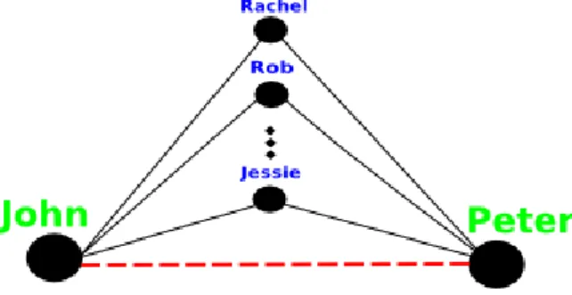
Figure 1.1: _{Link-Prediction used in ”People You May Know” recommendation in}

social network

Figure 1.1 shows an example of a traditional link-prediction method, which is called

the common-neighbors approach, and is used to recommend a new connection between

two people. In the depicted example, John and Peter (nodes of the graph) have a large

number of friends in common, because of that, there will be a high probability of them

knowing each other. Thus, they can be recommended to become friends in the social

network [9].

Mapping a Knowledge Base into a graph, allows literals (or instances) to be

repre-sented as nodes, and the relations between them (the predicates) to be reprerepre-sented as

edges. By simply applying link prediction to the graph we can infer new facts (not

previously present in the KB), as shown in Figure 1.1. But, if we also add ontological

information, for example information about the category of literals(instances), we can

use link-prediction techniques to extend the ontological model itself by finding possible

(18)

Figure 1.2 shows an example of how link-prediction can be used to find a possible new

relation to extend the original ontological model. The idea is similar to the one used to

find new facts (instances). The difference is that, counting edges is performed to groups

of nodes (from the same category), instead of to single nodes. Suppose, for instance, that

many nodes fromathlete category are related to nodes fromsport category. In addition,

suppose also that many nodes fromsportcategory are related to nodes fromsportsLeague

category. In such a scenario, a relation betweenathlete andsportsLeague categories can

be recommended, in this case the new relation could be named athletePlaysInLeague.

Figure 1.2: _{Link-Prediction applied to propose a new relation(}_{athletePlaysLeague}₎

1.1.2 Using Ontological Information to Find Implicit Knowledge

The main focus of our research is to investigate algorithms that would explore the use of

ontological information from an OKB to discover/extract implicit knowledge to augment

the original OKB itself. Starting from the definition of a simple OKB, such as presented

in this section (containing a set of categories, a set of relations among these categories,

instances of the categories and relations among the instances), we intend to proceed our

investigation and, also to propose approaches that can take advantage of such ontological

information to find new instances and also to extend the original ontology. By ontology

extension, we mean, the approach should focus also on finding new categories, as well

(19)

In the last subsection we presented some link prediction techniques examples that help

to find instances (Figure 1.1), and also to find new possible relations among categories

(Figure 1.2. Beyond that, we also want to explore, in this research work, techniques

to extend the ontology finding new categories. For that purpose, we could use for

example another graph mining task, called community detection[11], to divide or find

sub-categories for a given category already in the OKB (see Figure1.3for an example).

Figure 1.3: _{Athlete category, and the sub-groups (or sub-categories) that could be}

found with a community detection algorithm

Figure (1.3) shows an example of the task of find new categories (more specifically in this

case, sub-categories of an already existing category) through community detection. In

that figure, categoryathlete is present, and a community detection algorithm could find

soccer player,basketball player andbaseball player subcategories, using the topology of

the graph. We can observe that the nodes of these groups are dense connected to each

other, while the connection with node of other groups are very sparse.

1.2 Motivation

As we show in the beginning of this chapter, there is a lot of interest on building

large OKBs, generally, by gathering data from large corpora of text, websites such as

Wikipedia, or the web in general. Despite of the gigantic size of these OKBs, the

techniques used to extract knowledge from text (and from semi-strutured sources, like

(20)

implicit knowledge like human beings do. Thus, in addition to harvest these sources

to extract knowledge, a lot of implicit knowledge might be present in these OKBs,

which require inference-based algorithms to extract them. For example, consider the

two follow statements: “athlete Neymar Jr. plays on team Barcelona” and “athlete

Neymar Jr. plays on league Champions League”. Considering both statements, there

an implicit knowledge: “team Barcelona plays onleague Champions League”. A human

being probably would easily infer this implicit knowledge just by reading the first two

facts, but for a machine, it is not so easy to learn to infer it.

Considering its never-ending learning characteristics, NELL [1,7] is the main

motiva-tion of the research work here proposed. To build its continuously growing knowledge

base, NELL reads the web 24 hours per day, 7 days per week with two specific goals:

populate its own knowledge base and improve its learning abilities. A lot of research

was made to allow NELL performing these tasks based on different components (most

of the research is listed in its website3_{) and different theoretical approaches. NELL’s}

different components work together extracting information and learning from the web

(such as CPL and CSEAL), as well as from NELL’s own knowledge base (such as CMC

, RL and PRA[12–14]).

An important characteristic of an OKB (such as NELL’s) is that the ontology structure

itself can be considered to have specific patterns that can be used to infer new

knowl-edge, thus, to learn new categories or new possible relations to be added to the OKB,

would mean to obtain new knowledge. There are not many research works focused on

extending an ontology by finding implicit knowledge in the form of new categories and

new relations. Considering NELL, for example, there were not any active component to

extend its own ontology, before this work. There were, however, two components that

were previously designed to find new relations, namely Prophet[15] and OntExt[16], and

there was previous research on finding sub-categories for categories already present in

NELL’s own OKB based on the use of matrix factorization to cluster instances from

each category[17].

The first attempt to automatically extend NELL’s OKB was designed based on a distant

supervision learning approach and is named OntExt (Ontology Extender)[16]. OntExt

was designed to match all pairs of categories present in NELL’s ontology. For each pair

3

(21)

of categories, the idea is to gather all instances and use them to extract features from

an external textual corpus or database (such as subject-verb-object files, also known as

SVO). After that, OntExt creates a feature X feature co-occurency matrix and cluster

these pairs of features into groups. Each group is intended to represent a new possible

relation between two categories. The name of the relation would be the top ranked

feature in the group (or the group centroid).

The biggest problem with OntExt is that it does not scale well. To generate the features

co-ocurrency matrix, the complexity is O(n3_{), and to cluster the matrix, OntExt uses}

K-Means clustering algorithm[18], that has a considerably high complexity too. Because

of this high complexity issue, it wouldn’t be feasible to run OntExt for all category pairs

combinations in an acceptable time window, to make it iterative and never-ending like

NELL.

Prophet [15] was designed to be one of NELL’s ontology extension components. The

main idea behind Prophet is to map NELL’s own OKB into a graph structure, and then,

apply link-prediction techniques into the generated graph. It executes a link-prediction

task using a metric called extra-neighbors[15] to extend NELL’s ontology by finding

new possible relations. Also, Prophet can be used to find new instances of the proposed

relations and some possible misplaced facts present on the KB.

Prophet’s first implementation has some software engineering issues, like, it doesn’t scale

well if the input graph grows too much on the number of nodes and edges. Also, the

score for the proposed relations (in its first implementation) are not precise, thus a great

part of those proposed relations might not be correct. Another limitation is that the

first implementation was directly coded into NELL’s KB by SQL queries, having his use

restricted to NELL. Besides all of that, Prophet just points two categories that might be

related, and it doesn’t give a name to the relation and can’t tell if there is more than one

possible relation among the two related categories (e.g playedAgainst(athlete, athlete),

teammate(athlete, athlete)).

Based on the lack of ontology extension components to NELL (and also to other

OKB-based projects), the main goals of this research were, given an Ontological Knowledge

Base as input:

(22)

II Design and Implement an algorithm to find new categories in NELL’s OKB.

III Design and Implement an algorithm to find new facts for the OKB using the

On-tology Information.

1.3 Methodology

To accomplish all goals, we focused on a graph mining approach, so the main related

research works are Prophet[19] and PRA[12,13]. Another research that worth attention,

mainly for the ontology extension algorithms, is OntExt[16]. Besides the main focus

being on these three related works, other contributions reported on the literature were

also studied during our work.

To achieve goal I, a new version of Prophet was designed and implemented in C++ to

be more generic, allowing other projects to use it (we intend to let it freely available for

download in the web), and also more scalable than the original one. After that, a new

OntExt version was also created and integrated with Prophet to take advantage of their

complementary characteristics.

It is important to mention that, because of Prophet’s intrinsic characteristics, its

algo-rithm can be easily adapted to be used as an OKB inference method. In this sense,

if instead of focusing only on open triangles (as done in Prophet), we focus on closed

triangles, the algorithm can be adapted to generate first order inference rules from the

OKB. Thus, as a side effect of the re-implementation of Prophet, a new inference rule

extractor for OKBs was designed and implemented. Considering that the new inference

algorithm is also based on link-prediction graph mining techniques, it is called theGraph

Rule Learner - GRL. Therefore, in spite of not having the main goal of proposing a new

OKB inference algorithm, this masters work contributes GRL as a side effect of its first

goal, and defined as the third goal.

To achieve the second goal, an algorithm that clusters each category to find

sub-categories was created. This algorithm is similar to OntExt, because it will build a

features-based matrix to cluster the instances of the given category to find new

(23)

very similar to Prophet, was created to find patterns that are present at the graph to

create inference rules to extract implicit facts.

A sumarization of the methodology is presented below:

• Investigation of past research works about ontology knowledge bases, and ontology

extension algorithms;

• Analysis of previous works about Prophet[15, 19] and OntExt[16] and Chunlei’s

category extension approach [17];

• Design and implementation of a new version of Prophet, as well as a new version

of OntExt, and integrate both of them to achieve goal I;

• Investigation the use of elements of OntExt and Prophet (like the Extra-Neighbors

Index) to create algorithms to achieve goal II and III;

• Implementation and validation of the algorithms designed to solve goals I, II and

III;

• Integration of these algorithms to run within NELL.

1.4 Organization

In the Chapter2, the review of the literature for the research is present, containing also

one section briefly presenting NELL with its initial architecture. Chapter3presents the

Ontological Network structure and how to map an Ontological Knowledge Base using

it. This structure is used in the next chapters to explain and exemplify our projects:

in Chapter 4 the on that finds new facts, in Chapter5 the one that finds new relations

and in Chapter 5.5the one that finds new categories, all of them using the ontology to

find implicit knowledge. After that in Chapter 5.7 we present some future extensions

to our projects and following in Chapter 5.10 the final conclusion. Next to that are an

Appendix presenting some results of the projects and following that the bibliography

(24)

Chapter 2

Literature Review

In this chapter we present the background theories and methods important to ours

masters project, and also Nell’s architecture and how its OKB is defined.

2.1 Background

As aforementioned, our proposal is to investigate, design and implement algorithms to

(semi)automatically extend OKBs. Our intention is to explore the possibility of mapping

an input OKB into a graph, and then use graph mining techniques. The main approach

in which our research is based on is link-prediction. In the last years a large number of

methods has been proposed on this topic, and a review on those can be seen in [20].

Most link prediction methods are based on graph structural properties [21] in which the

goal is to assign connection values, calledscore(u;w), to pairs of nodeshu, wibased on a

graphG. Traditionally, the assigned scores are later ranked in a list in decreasing order

of score(u;w), and then, predictions are made according to this list.

For a node uin the graph G, let Γ(u) denote the set of neighbors ofu inG. A number

of link prediction approaches are based on the idea that two nodes in G (e.g u and w)

are more likely to link to each other, in the future, if their sets of neighbors Γ(u) and

Γ(w) largely overlap.

The most straightforward implementation of this link-prediction idea is the

common-neighbors metric [9], under which thescores are defined asscore(u;w) :=|Γ(u)∩Γ(w)|.

(25)

Chapter 2. Literature Review 10

Common-neighbors predictor captures the basic notion, inspired in social networks, that

two strangers who have a common friend may be introduced by that common friend and,

thus, become friends themselves. When analyzing hisintroduction act in a graph-based

context, it has the effect of “closing a triangle” in the graph and feels like a common

mechanism in real life [22].

Link prediction can make use not only of graph structural information but also relational

characteristics, for example attributes related with graph’s node as presented in [23].

This kind of approach is more used in relational or multi-relational learning [8,24–26].

Besides the amount of different approaches described in the literature for the link

predic-tion task, results presented in [27] indicate that the simplest measure, namely common

neighbors has, in general, the best overall performance. Also, this very simple approach

has the property of making it easy to calculate a cumulative number of neighbors if

nodes were associate to a class.

Another technique that we widely use in this research is clustering. A review on those

can be seen in [28]. Clustering algorithms are mostly used to solve unsupervised learning

problems[29], so, as every other problem of this kind, it deals with finding a structure in

a collection of unclassified data. A loose definition of clustering algorithm could be “the

process of organizing objects into groups whose members are similar in some way”, so, a

cluster is a collection of objects which are “similar” between them and are “dissimilar”

to the objects belonging to other clusters.

One of the most famous clustering algorithm is called k-means[18]. It works iteratively

creating centroids(data points in which each feature is the mean of the group’s data

points feature) them relocating the data points to the closest centroid, until is error

is lower to a given threshold. Generally, k-means is used to cluster data points with

numerical features, so the most common distance functions used is Euclidean Distance

or Manhattan distance[30]. The distance function can be different to work with discrete

data (like text).

We also talk a lot about rule learners and inference rules. An inference Rule (or just

rule) is a logical form, consisting of a conclusion r, and premises p1, p2, ..., pn. One

possible representations is r ⇐= p1 ∧p2 ∧...∧pn. The premises and the conclusion

(26)

return true or false. For example. we can have the following rule: grandf ather(A, C)⇐=

f ather(A, B)∧f ather(B, C), that indicates that ifAis father ofB, and B father ofC,

thenA is grandfather of C.

2.2 NELL

The Read The Web project’s system is called the Never Ending Language Learner

(NELL) [1]. NELL is a long life learning system that reads the web 24h a day, 7 days

a week, since January, 2010. In each iteration NELL main goals are to learn new facts,

extends its ontology finding new categories and relations, and to improve its learning

abilities.

NELL’s knowledge Base can be considered an ontological knowledge base (OKB):

com-posed by categories (e.g. person, sportsTeam, fruit, emotion, etc.) and relations

(e.g. musicianPlaysInstrument(musician, instrument)). Category instances (e.g.

per-son(Barack Obama), sportsTeam(Pittsburgh Steelers)), as well as relation instances (e.g.

athletePlaysFroTeam(Ward, Pittsburgh Steelers)) are facts. NELL’s OKB is divided in

two main types of facts,Candidate Facts, are those facts that NELL has weak evidence

of their truth, but not enough to be confident about them. On the other hand,Beliefs

are facts that NELL is confident enough about their truth.

(27)

Figure 2.1 shows the core structure of NELL, its OKB and the main four components

that read the web and transform the information available in knowledge. This four

components are briefly describe below:

CPL: extracts knowledge using contextual patters like “mayor of x” and “X plays for

Y”;

CSEAL: semi-structured extractor which queries the Internet with sets of beliefs from

each category and relation, and then mines lists and tables to extract novel

in-stances of the corresponding predicate;

CMC: based on simple set of binary L2-regularized logistic regression models which

classify noun phrases based on various morphological features (words,

capitaliza-tion, affixes, parts-of-speech, etc.);

RL: first-order relational learning algorithm similar to FOIL, which learns probabilistic

Horn clauses from the ontology. It is possible to compare it to a procedure that

identifies sets of relations (sets of three relations) that are already present in the KB

and can be connected in a transitivity-based approach such as: if relation1(A,B)

and relation2(B,C) both hold, then relation3(A,C) also holds.

The main motivation of this whole Masters research project is NELL and all of the

algorithms that are presented in the next chapters are intended to work as NELL’s

components, automatically and iteratively finding new facts (such as the ones presented

(28)

Chapter 3

Ontological Networks

In this chapter we will present the Ontological Network structure, that was designed to

formally map an ontological knowledge base (OKB) into a graph. This structure was

designed mainly to help in the design and description of the algorithms of the projects of

this research. But we believe that is can also be very helpfull to other recent researches

that uses OKBs.

There are libraries such as graphOnt[31] that maps ontologies into graphs for better

visualization or analysis, and also a class called OWLGraphWrapper1 _{from OWLTools.}

These libraries are very useful to directly apply some graph-like operations over

onto-logical knowledge bases, but none of them described a formal definition.

First there’s a definitions section to formally present some notations that will be used in

this chapter and in the algorithms in the next chapters either, then we formally define

an ontological KB to them formally define an ontological network and the mapping

process. We also present some examples in this chapter that will be used to exemplify

the algorithms in the next chapter either.

3.1 Base Definitions

Let G = (V, E) be an undirected graph with a set of nodes V and a set of edges E.

Γ(u) :={v∈V :∃{v, u} ∈E} of nodeu is defined to be the set of nodes in V that are

1

http://owltools.googlecode.com/svn/trunk/docs/api/owltools/graph/OWL GraphWrapper.html

(29)

Chapter 3. Ontological Networks 14

adjacent to u. The number of common neighbors between two nodes (u and v) can be

defined asℵ(u, v) =|Γ(u)∩Γ(v)|.

A closed triangle ∆(u, v, w) of a graphG= (V, E) is a set of three complete connected

nodes where u, v, w ∈ V and ∆(u, v, w) = {< u, v >, < v, w >, < w, u >} ∈ E. An

open triangle Λ(u, w) of a graph G= (V, E) is three connected node where Λ(u, w) =

{(u, v),(v, w)} ∈ E∧ {u, w} ∈/ E. The ∆c(c1, c2, c3) represents all the closed triangles composed by node’s of categories c1, c2 and c3 and Λc(c1, c2) represents all the open triangles composed by node’s categories of c1 and c2 (in this case, the middle nodes

categories doesn’t matter). Any ∆c is called a closed triangles category group and

any Λc is called a open triangles category group. The cu of a node u is the set of

the categories thatu belongs to.

3.2 Defining an Ontological Knowledge Base (OKB)

To define an ontological network created from an OKB, we need to formally define an

OKB first. In this section an OKB format we call OKB2 is defined. To do so it is used

predicate logic elements.

Definition 1. An Ontological Knowledge Base OKB2 = (C, H, R, I) is composed by

four components: a set of categories(C), a set (H) of predicates “ako(a kind of)” that

express the hierarchy against the categories, a set (R) of predicates that express relation

among the categories.

• ∀predicates p(t1,t2) ∈H, Rthe arity of p is 2 (p/2) andt1, t2 ∈C;

• The predicate “ako”∈Hare transitive: ifako(t1, t2),ako(t2, t3)∈H,thenako(t1, t3)

∈H;

• It must not exist predicates with equal terms in H: ako(t, t)∈/H;

At last, a set of instances(I) of the categories(C) and relations(R). The instances set(I)

are the facts of theOKB2. The set (I) can be divided in two subsets, the categorization

set and the relational set (I =Ic∪Ir)

• The categorization set (Ic) is composed by predicates pc(t) with names of the

(30)

• The relational set (Ir) is composed by predicatespr(t1, t2) such that: pr(c1, c2)∈R and c1(t1), c2(t2)∈Ic.

The number 2 in the name of our OKB model (OKB2_{) was chosen because all of the}

relations on this model can only have arity 2. Above we present an example to better

illustrate howOKB2 _works.

Example 1. Consider an ontological knowledge base OKB_social2 = (C, H, R, I) used to store data from a social network that have different types of relations.

• C={Person, MaleP, FemaleP};

• H={ako(MaleP, Person), ako(FemaleP, Person)}

• R={friends(Person, Person), fatherOf(MaleP, Person), motherOf(FemaleP,

Per-son), descendant(Person, PerPer-son), relationship(MaleP, FemaleP), relationship(FemaleP,

MaleP)}

• I = Ic ∪Ir = {Person(Lucas), MaleP(Lucas), Person(Jose), MaleP(Jose),

Per-son(Raquel), FemaleP(Raquel), Person(Julia), FemaleP(Julia), Person(Vinicius),

MaleP(Vinicius), Person(Leo), ...} ∪ {friends(Lucas, Leo), friends(Vinicius, Leo),

friends(Julia, Raquel), relationship(Lucas, Julia), relationship(Raquel, Jose),

rela-tionship(Jose, Raquel), descendant(Lucas, Jose), descendant(Vinicius, Jose),

de-scendant(Vinicius, Raquel), fatherOf(Jose, Lucas), motherOf(Raquel, Lucas),

moth-erOf(Raquel, Vinicius), ...}

3.3 Defining an Ontological Network (

N

o

)

In this subsection we’ll define an ontological network (No) created from an arbitrary ontological knowledge base OKB2.

Definition 2. An Ontological Network No _{= (G}

m, Gi) is composed by two graphs, an

ontological model graph (Gm) and an ontological instances graph (Gi).

An Ontological Model Graph Gm = (Vm, Em) has the same purpose of the model parts

on the OKB2, to determine the categories that the instances can be and the possible

(31)

that represents categories, and the set of edges Em is composed by labeled edges that

represents a relation name.

Definition 3. Given an Ontological Knowledge BaseOKB2 = (C, H, R, I), an

Ontologi-cal Model GraphGm= (Vm, Em) can be created to map the ontological model ofOKB2

such as:

• Vm ≡C: ∀c∈C ∃v∈Vm |v.label=c;

• Em ≡H∪R: ∀p(t1, t2)∈H∪R∃e∈Em |e=p < t1, t2>;

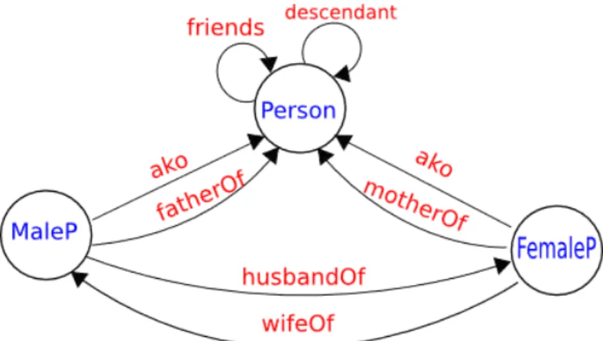
To better illustrate an ontological model graph, above an example is present, mapped

from the OKB2 of Example 1.

Example 2. Given the OKB2

social presented at Example 1, the ontological model graph

Gm= (Vm, Em) mapped by it would be:

• Vm ={P erson, M aleP, F emaleP};

• Em = {ako < M aleP, P erson >, ako < F emaleP, P erson >, f riends< P erson,

P erson >, f atherOf < M aleP, P erson >,...};

Figure 3.1: _{Ontological Model Graph Example}

The Figure 3.1 is the graphic representation of the graph presented in Example 2.

An Ontological Instances GraphGi= (Vi, Ei, X) is the graph that will be the network of

the instances of the KB. The set of nodesVi is composed by labeled nodes, representing

the instances (the parameters of the predicates∈I). The set of edgesEi is composed by

labeled edges that represents relations among two instances. The setX is the category

(32)

Definition 4. Given an Ontological Knowledge Base OKB2 = (C, H, R, Ic ∪Ir) and

Ontological Model GraphGm = (Vm, Em) mapped fromOKB2, an ontological instances

graphGi = (Vi, Ei, X) can be created to map the instances ofOKB2 such as:

• ∀pc(t)∈Ic ∃v ∈Vi|v.label =t;

• Ei ≡Ir: ∀pr(t1, t2)∈Ir ∃e∈Ei |e=pr < t1, t2 >;

• X≡Ic: ∀pc(t)∈Ic ∃x∈X |x= (t, pc);

To better illustrate an ontological instances graph, above an example is present, mapped

from the OKB2 _{of Example 2.}

Example 3. Given the OKB2

social presented at Example 1, the ontological instances

graphGi = (Vi, Ei) mapped by it would be:

• Vi ={Lucas, Jose, Raquel, Vinicius, Leo, Julia, ...};

• Ei ={friends(Lucas, Leo), descendant(Lucas, Jose), fatherOf(Jose, Vinicius),

re-lationship(Lucas, Julia), ...};

• X = {(Lucas, Person), (Lucas, MaleP), (Raquel, Person), (Raquel, FemaleP),

(Leo, Person), ... }

(33)

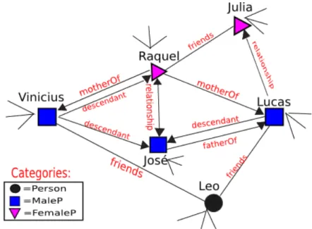
The Figure 3.2 is the graphic representation of the portion of the graph presented in

Example 3 (mapped from I of Example 1). The categorization setX is represented by

the node colors and shapes.

An alternative format for aNo_{, that can be also very interesting to apply graph-mining}

algorithms, is a format with just one unified graph:

No′ = (Vm∪Vi, Em∪Ei∪X)

In No′

there is just one graph, unifying the ontological model with the instances. In

practice this network generally will look like a small world network[32], with the category

nodes being the hubs.

We use anOKB2 to build (and define) and Ontological Network, but anNo _{can exists}

by itself, and not just mapped from an OKB. Actually, OKB2 _and _N

o are equivalent

models. It is possible to represent anyone of the two of them using the other.

3.4 Setting a second example

Now that OKB2 and No models are already defined, in this section a second example is presented. It will be an OKB containing sport-related data. This example and the

social network example will both be used in the next chapters to exemplify the algorithms

created in this project. OKB2andNo_{will be presented to better exemplify the mapping}

process.

3.4.1 OKB_sports2

Consider an ontological knowledge base OKB_sports2 = (C, H, R, I) used to store data from knowledge related to sports:

• C={Athlete, SportsTeam, SportsLeague, Stadium, Continent};

• H={} (empty)

• R={athletePlayedAtCountry(Athlete, Contry), athletePlaysForTeam(Athlete,

(34)

teamPlaysLeague(SportsTeam, SportsLeague),

teamPlayedAtCountry(SportsTeam, Country), leagueUsesStadium(SportsLeague,

Stadium), stadiumLocatedAtCountry(Stadium, Contry),

athletePlayedAtStadium(Athlete, Stadium),

leaguePlacedAtCountry(SportsLeague, Country)}

• I =Ic∪Ir ={Athlete(Neymar Jr,), Athlete(Jorge Valdivia), Country(Spain),

Country(Brazil), Stadium(Camp Nou), Stadium(Vila Belmiro), Stadium(Allianz

Pq) SportsTeam(Barcelona), SportsTeam(Palmeiras), SportsLeague(Champions

League), SportsLeague(Brazillian Cup), athletePlayedAtStadium(Neymar Jr.,

Vila Belmiro), athletePlayedAtStadium(Jorge Valdivia, Vila Belmiro),

athletePlaysForTeam(Neymar Jr., Barcelona), athletePlaysForTeam(Jorge

Valdivia, Palmeiras), athletePlayedAtCountry(Neymar Jr., Spain),

athletePlayedAtCountry(Neymar Jr., Brazil), athletePlayedAtCountry(Jorge

Valdivia Brazil), stadiumLocatedAtCountry(Camp Nou, Spain),

stadiumLocatedAtCountry(Vila Belmiro, Brazil),

stadiumLocatedAtCountry(Allianz Pq, Brazil), teamPlaysLeague(Barcelona,

Champions League), teamPlaysLeague(Palmeiras, Brazillian Cup),

teamPlayedAtCountry(Barcelona, Spain), teamPlayedAtCountry(Palmeiras,

Brazil), leagueUsesStadium(Brazillian Cup, Allianz Pq.),

leagueUsesStadium(Champions League, Camp Nou),

leaguePlacedAtCountry(Champions League, Spain),

leaguePlacedAtCountry(Brazillian Cup, Brazil), ...}

3.4.2 N_sportso = (Gm, Gi)

Given theOKB_sports2 , the ontological model graphGm = (Vm, Em) mapped by it would

be:

• Vm ={Athlete, SportsT eam, SportsLeague, Stadium, Continent};

• Em = {athletePlayedAtCountry<Athlete, Contry>,

athletePlayedForTeam<Athlete, Team>, athletePlaysForTeam<Athlete, Team>,

athletePlayedAtStadium<Athlete, Stadium>, teamPlaysLeague<SportsTeam,

(35)

stadiumLocatedAtCountry<Stadium, Contry>,

athletePlayedAtStadium<Athlete, Stadium>};

Figure 3.3: _{Ontological Model Graph}_G_m_{of Sports Network}

Given theOKB2

sports, the ontological instances graphGi = (Vi, Ei) mapped by it would

be:

• Vi ={Neymar Jr., Jorge Valdivia, Spain, Brazil, Camp Nou, Vila Belmiro,

Allianz Pq, Palmeiras, Barcelona, Champions League, Brazillian Cup, ...};

• Ei ={athletePlayedAtStadium<Neymar Jr., Vila Belmiro>,

athletePlayedAtStadium<Jorge Valdivia, Vila Belmiro>,

athletePlaysForTeam<Neymar Jr., Barcelona>, athletePlaysForTeam<Jorge

Valdivia, Palmeiras>, athletePlayedAtCountry<Neymar Jr., Spain>,

athletePlayedAtCountry<Neymar Jr., Brazil>, athletePlayedAtCountry< Jorge

Valdivia Brazil>, stadiumLocatedAtCountry<Camp Nou, Spain>,

stadiumLocatedAtCountry<Vila Belmiro, Brazil>, stadiumLocatedAtCountry<

Allianz Pq, Brazil>, teamPlaysLeague<Barcelona, Champions League>,

teamPlaysLeague<Palmeiras, Brazillian Cup>,

teamPlayedAtCountry<Barcelona, Spain>, teamPlayedAtCountry<Palmeiras,

Brazil>, leagueUsesStadium<Brazillian Cup, Allianz Pq.>,

(36)

leaguePlacedAtCountry<Champions League, Spain>,

leaguePlacedAtCountry<Brazillian Cup, Brazil>, ...};

• X ={(Neymar Jr., Athlete), (Jorge Valdivia, Athlete), (Spain, Country),

(Brazil, Country), (Camp Nou, Stadium), (Vila Belmiro, Stadium), (Allianz Pq,

Stadium), (Barcelona, SportsTeam), (Palmeiras, SportsTeam), (Champions

League, SportsLeague), (Brazillian Cup, SportsLeague), ... }

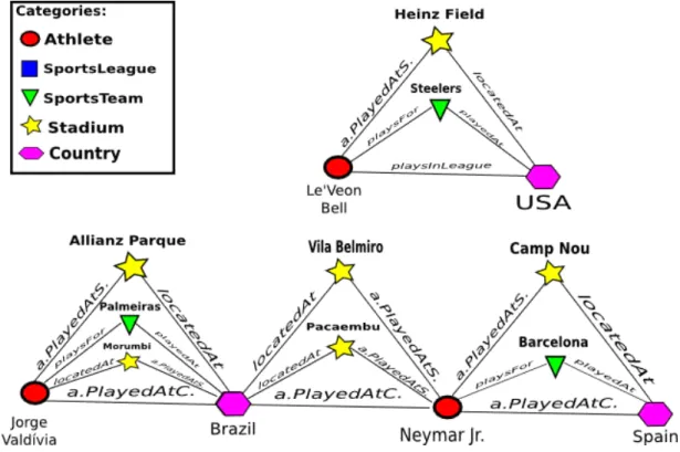
Figure 3.4: _{ontological instances graph}_G_i _{of Sports Network}

In this section we presented the sports OKB OKB_sports2 then we formally present the Ontological NetworkNo

sports with both in text and in figures to the better visualization

of it. One interest observation is that mostly of the projects that uses OKBs such as

NELL, there are a lack of facts (and some wrong facts either). Observing theNo sports

example, a human being might know that Neymar Jr. played at Camp Nou lots of times

because it plays for Barcelona and Camp Nou is Barcelona’s home stadium, but this fact

is missing. This is very common in the OKB of a continuous learning program such as

NELL because it cannot read everything instantaneously, it will be learning more and

(37)

Chapter 4

Finding new facts

Even in a never-ending learning approach, the question of how to develop methodologies

to help populating OKBs with facts and improving their coverage is still a challenge [14].

Thus, the use of a rule-based inference approach (here called Rule Learner - RL) can

have relevant impact in the KB population task. In general, the goal of a RL is to induce

inference rules from structured or unstructured data[33].

An Inference Rule (or just rule) is a logical form, consisting of a conclusion r, and

premises p1, p2, ..., pn. One possible representations is r ⇐= p1 ∧p2 ∧...∧pn. The

premises and the conclusion are literals that can be predicates (p), a logical function

p(x1, x2, ..., xn) that can only return true or false. For example. we can have the following

rule: grandf ather(A, C) ⇐= f ather(A, B)∧f ather(B, C), that indicates that if A is

father ofB, andB father of C, then Ais grandfather of C.

In the context of graphs mapping knowledge bases we can use techniques similar to

link-prediction to find patterns of closed triangles instead of open triangles. Following

there’s an example using the model of No _{proposed to explain how a RL can use these}

patterns to find inference rules.

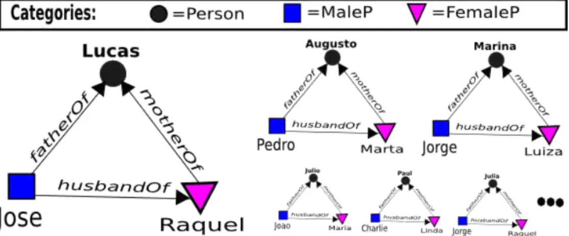
If we create an algorithm that exploits patterns of close triangles, in a graph based on

three category nodes and the relations among them, it could be applied to the graph

of the Figure4.1 and it could find ∆M aleP, P erson, F emaleP as an interesting group

to promote a rule. It would happen because there are a lot of triangles with these 3

categories in the same “position” in terms of relations. In this case, the following rule

could be proposed:

(38)

Chapter 4. Finding new facts 23

Figure 4.1: _{Example of a pattern of closed triangles between MaleP, Person and}

FemaleP

husbandOf(M aleP :X, F emaleP :Y)⇐=

f atherOf(M aleP :X, P erson:Z)∧motherOf(F emaleP :Y, P erson:Z)

The rule says that if a MalePXis father of a Person Zand a FemalePY is the mother

of the same PersonZ, then MaleP Xis the husbandOf FemaleP Y.

This rule can be used to find new instances of the relation husbandOf to the No social,

adding edges toGi (the same thing as adding facts to the OKB).

4.1 The Graph Rule Learner

The Graph Rule Learner (GRL) is an algorithm designed to extract inference rules

from ontological knowledge bases. GRL uses a link-prediction metric called

extra-neighbors[15] to rank possible rules, and also to determine the antecedents and

con-sequents of each induced rule.

Rule induction from data is not a novel task and many different approaches have been

proposed. Due to space constraints, in this section we focus on more recent approaches

and which are closely related to GRL. The Online Rule Learner (ORL) [33] mines

inference rules from explicit information extracted from large corporas using automated

information extraction (IE) systems [34,35]. ORL is similar to GRL in the sense that it

(39)

ORL uses the topology of the created graph to extract rules, instead of link prediction

techniques used in GRL. The Universal Schema proposed in [36] focuses on the benefits

of using latent features for increasing coverage of KBs. Key differences between that

approach and the one proposed in the work described in our paper include our use of

graph-based link prediction measurements as opposed to surface-level patterns in theirs,

and also the ability of the proposed GRL method to generate useful (and comprehensible)

inference rules which is beyond the capability of the matrix factorization approach.

A traditional approach to extract inference rules is the inductive logic programming

(ILP), which deduces rules from ground facts. According to [37], current ILP systems

cannot be applied to KBs who gathers data from web with a large scope of categories

(anything in the world), such as NELL, mainly because they usually require negative

statements as counter-examples, and these projects just hold instances that they consider

correct or have some confidence1. Also, the ILP-based approach don’t scale to the huge amount of data that these kind of KBs store.

Regarding NELL’s, when considering its KB as input to induce inference rules, there

are other previously proposed approaches. In [38] a Markov Logic approach is used to

allow inference over subsets of categories and relations. PRA[12], and the Latent PRA

[14] and Prophet[15] are graph-based approaches. PRA (Path Ranking Algorithm) uses

a combination of constrained, weighted, random walks through NELL’s KB graph to

reliably infer new beliefs for it’s KB. PRA performs such inference by automatically

learning semantic inference rules over the KB [13]. Latent PRA proposes the addition

of edges labeled with latent features mined from a large dependency parsed corpus of

500 million Web documents to improve performance of previous PRA. Recently the

PRA was combined with a vector space representations of surface forms to increase its

performance and be capable of execute with the sparsity of textual representations from

surface text[39].

Prophet, is not an inference component. However, it is important to mention this

component because GRL approach is closely related to Prophet graph mining approach.

Differently from PRA approaches (which are based on random walks), Prophet counts

on NELL’s KB (represented as a graph) as input to (semi-)automatically extend NELL’s

initial KB. As aforementioned, Prophet does not induce inference rules from the KB,

1

(40)

but the same link prediction idea used in Prophet to extend the KB, is adapted in GRL

to induce inference rules.

According to [33], there are two problems with most of the existing inference rule

learn-ers: [40] [41] [42] [43], they do not scale when based on large corpora and they tend to

assume that the training data is largely accurate and complete. However, to be coupled

to a never-ending learning system, such as NELL, a RL must overcome both issues. It

happens mainly because NELL’s KB is continuously growing and continuously being

updated and revised by NELL’s components.

GRL assumes that the training data is mostly (but not completely) accurate and

com-plete. However, it is not a problem if the KB is either imperfect, or incomcom-plete. Actually,

link prediction algorithms assume that the missing links are due to the KB evolution

in the near future, thus it is currently incomplete. To take advantage of more accurate

knowledge, GRL limits its learning process to the specific part of NELL’s OKB called

the set ofbeliefs (composed just by high confidence facts). Regarding scalability, GRL

scales with large graphs (the same as large KB’s), using a graph disk structure called

GraphDB-Tree [44].

4.1.1 GRL Algorithm

GRL needs an ontological instances graph as input, and its output is a list of induced

inference rules.

Algorithm 1 The GRL

Require: Gi= (V, E, X)

Ensure: List of Inference Rules 1: Find all ∆(u, v, w) in Gi

2: for allclosed triangle ∆(u, v, w)do

3: Calculateℵ(u, v),ℵ(v, w) andℵ(w, u) 4: Group ∆(u, v, w) in ∆c(cu, cv, cw)

5: Group Λ(u, v) in Λc(cu, cv), Λ(v, w) in Λc(cv, cw) and Λ(w, u) in Λc(cw, cu)

6: end for

7: for allΛc(ci, cj)do

8: Calculateℵc(ci, cj)

9: end for

10: for all∆c(cu, cv, cw)do

11: Find the category pair with highestℵc:

(ci, cj) =M AX(ℵc(cu, cv),ℵc(cv, cw),ℵc(cw, cu))

12: if ℵc(ci, cj)≥ξthen

13: Validate the rule: rcicj(ci, cj)⇐=rcick(ci, ck)∧rckcj(ck, cj)

14: end if

(41)

Inline 1, GRL finds and lists all closed triangles ∆(u, v, w) present in graphGi. Then,

for each triangle, the number of neighborsℵbetween each pair of nodes is calculated (e.g

ℵ(u, v)), and grouped in the respective open triangle category group Λc2 (e.g Λ(cu, cv)).

The closed triangle is also grouped in the closed triangle category group ∆c(cu, cv, cw). In

line 8, for each open triangle category group Λc(ci, cj), the number of extra neighbors

ℵc is calculated. ℵc is the sum of the ℵ − 1 of all instances Λ(i, j) in the group. If

ℵc(ci, cj) = 0 it indicates that all pair of nodes Λ(i, j) in the group have only one

neighbor in common. In line 11, for each closed triangle category group ∆c(cu, cv, cw),

the pair of categories with the highest extra neighbors value ℵc will be selected (e.g

(cu, cv)). Then, if the extra neighbor value of this pair is greater or equal than a given

thresholdξ, the rulercucv(cu, cv)⇐=rcucw(cu, cw)∧rcwcv(cw, cv) is validated. One literal

rcxcy(cx, cy) indicates a relation(predicate)rcxcy ∈Ec between the categoriescx and cy,

and its parameters must be instances of categories cx and cy respectively.

4.1.2 Example

In Figure 4.2, a simple example of the GRL algorithm for an arbitrary graph is

pre-sented.

We have the closed triangle category group ∆c (Athlete, Stadium, Country), and its

six instances:

∆(N eymarJr., CampN ou, Spain),

∆(N eymarJr., V ilaBelmiro, Brazil),

∆(JorgeV aldivia, AllianzP arque, Brazil)and

∆(N eymarJr., P acaembu, Brazil),

∆(JorgeV aldivia, M orumbi, Brazil),

∆(Le′

veonBell, HeinzF ield, U SA).

2

(42)

Figure 4.2: _{GRL running example}

Now we have to pick the pair of categories among this three categories with the greatest

extra-neighbor value, and the pair with the greatest is Athlete and Country:

ℵc(Athlete, Country) =ℵ(N eymarJr., Brazil)

+ℵ(N eymar, Spain)

+ℵ(JorgeV aldivia, Brazil)

+ℵ(Le′

veonBell, U SA)

− |Λc(Athlete, Country)|

ℵc(Athlete, Country) = 2 + 2 + 3 + 2−4 = 5≥ξ(ξ = 5)

The other two pairs have a lower EN value (ℵc(Stadium, Country) =ℵc(Stadium, Athlete) =

0). If we consider a threshold equals to five (ξ = 5) then we can validate the rule among

the three categories (Athlete, Stadium and Country) with Athlete and Country being

(43)

three categories of the group, the rule will be:

athleteP layedAtCountry(Athlete, Country)⇐=

athleteP layedAtStadium(Athlete, Stadium))

∧stadiumIsLocatedAtCountry(Stadium, Country)

The rule says that if an athleteXplayed at a StadiumYand this StadiumY is located

at Country Z, then athlete X already played at Country Z. The generalization of the

rule to X,Y and Z process will be present in a subsection above.

Figure 4.3: _{Applying a rule to infer new facts}

After GRL found a rule, then it is possible to use the rule to infer new facts to

the input OKB. Let’s suppose we have open triangles Λ(N eymarJr., England) and

Λ(M essi, M essi) (see Figure4.3), using the rule GRL just discover it is possible to add

two facts to the OKB (athleteP layedAtCountry(N eymarJr., England) andathleteP layedAtCountry(M

Spain)), closing the triangles because we have:

1.athleteP layedAtStadium(N eymarJr., S.Bridge)

∧stadiumIsLocatedAtCountry(S.Bridge, England)

=⇒athleteP layedAtCountry(N eymarJr., England)

2.athleteP layedAtStadium(M essi, CampN ou)

∧stadiumIsLocatedAtCountry(CampN ou, Spain)

(44)

In this example, there is also another possible closed triangle category group: ∆c

(Athlete, SportsT eam, Country) but no pair of categories (Λ) that belongs to these

groups achieves an ℵc greater or equal to 5 in this example.

4.1.3 Multi Relation CTCGs

In a closed triangle category group, more than one triple of relations is possible, let’s

sup-pose that the relation athleteP layedAgainstT eam <athlete, SportsT eam > is added

to our sports ontological network (No

sports) with the edges playsAgainst< N eymarJr.,

Real M adrid > and playedAt< Real M adrid, Spain >. With this changes, the graph

of Figure4.2will be changed: see at Figure4.4for the changes.

Figure 4.4: _{GRL example for multi relation CTCGs}

If those two edges exist, then the closed triangle ∆c (Athlete, SportsT eam, Country)

will have a pair for which ℵc is higher than the threshold:

ℵc(Athlete, Country) =ℵ(N eymarJr., Spain)

+ℵ(JorgeV aldivia, Brazil)

+ℵ(Le′

veonBell, U SA)

− |Λc(Athlete, Country)|

(45)

We can then, validate a rule having categories Athlete and Country as the head, but

we have multiple relations among the three categories of this group (see instances:

∆ (N eymarJr., Barcelona, Spain) and ∆ (N eymarJr., RealM adrid, Spain)). The

triple of relations for the first one is (athletePlaysForTeam, teamPlayedAtCountry,

ath-letePlayedAtCountry) and for the second is (athletePlayedAgainstTeam,

teamPlayedAt-Country, athletePlayedAtCountry). Having multiple triples of relations inside the same

group, indicates that multiple rules can be created, so it is necessary to decide how to

choose among these multiple triples of relations.

To solve the problem of choosing one rule from all the possible ones (for a single group)

GRL, for now, just counts the occurrence of each triple inside a closed triangle category

group and pick just the one that occurred more frequently. For the example above, we

have the two rules:

(a) athleteP layedAtCountry(Athlete, Country)⇐=

athleteP laysF orT eam(Athlete, SportsT eam))

∧teamP layedAtCountry(SportsT eam, Country)

(b) athleteP layedAtCountry(Athlete, Country)⇐=

athleteP layedAgainstT eam(Athlete, SportsT eam))

∧teamP layedAtCountry(SportsT eam, Country)

Rule (a) relations combination occurred three times - with (Neymar Jr., Barcelona,

Spain),(Le’Veon Bell, Steelers, USA) and (Jorge Valdivia, Palmeiras, Brazil), while rule

(b) relations combination occurred just once, with (Neymar Jr., Real Madrid, Spain).

Because of that, rule (a) will be validated and rule(b) will be discarded. In this case

rule (a) makes more sense than rule (b), but in some cases more than one rule could be

correct, and because of that, in the future we plan to explore other possibilities to pick

up rules in case of Multi Relation CTCGs.

4.1.4 Grouping and Ranking Rules

When using NELL’s KB (as well as any other OKB) as input, it is expected to find several

(46)

is expected mainly because in such OKBs, there are hierarchy among categories and

multi-categorized instances. See the example below of GRL’s output on NELL’s graph:

teamP laysSport(sportsT eam, sport)⇐= athleteP laysSport(sport, athlete)

∧athleteP laysF orT eam(athlete, sportsT eam)

teamP laysSport(sportsT eam, sport)⇐= athleteP laysSport(sport, personAsia)

∧athleteP laysF orT eam(personAsia, sportsT eam)

teamP laysSport(sportsT eam, sport)⇐= athleteP laysSport(sport, personU sa)

∧athleteP laysF orT eam(personU sa, sportsT eam)

Following along these lines, a grouping and ranking process is applied on the GRL

output. This process consists on simply grouping all rules, which share repeated

predi-cates, in one single generic rule with variables (X,Y andZ) as parameters, and ranking

these rules by the number of occurrences on GRL’s output list. After this process, we

can use this rank to increase confidence in some of the rules. Experiments over this

process are present in Section 5.6.2.

4.1.5 GRL Implementation

One common problem when implementing a graph mining algorithm is scalability, mainly

when working with graphs having a growing number (from hundreds to millions and

sometimes billions) of nodes and edges. To cope with this scalability issue, GRL stores

the graph representation in disk using a structure called GraphDB-Tree [44].

The GraphDB-Tree is a structure created for fast storage and recovery of a graph on

secondary memory. The complexity to recover the neighbor list for any node is O(1),

so this structure is very efficient to graph algorithms that uses just the locality of the

nodes (e.g., find graph cliques – such as triangles -, calculate Adamic/Adar and Jaccard

index, etc).

To achieve high performance in the node’s locality algorithms, GraphDB-Tree stores the

graph partitioned in disk pages, and the entire set of nodes being numeric, sorted and

(47)

does not have such specific characteristics (sorted numeric nodes), so a preprocessing

process is necessary before the storage on GraphDB-Tree.

Figure 4.5: _{GRL Execution Diagram}

InFigure 4.5, we show a simple diagram of GRL implementation: It receives as input

an OKB file (mapped as a graph), pre-processes the file and stores the graph in the

GraphDB-Tree data structure. Then, GRL initiates its execution querying for closed

triangles in the graph and grouping then into their respective category groups. After

all triangles were found, extra neighbors values are calculated and GRL validates the

extracted rules based on the given threshold value. The output will be the list of inference

rules.

4.2 Experiments

In this section we show some results (inference rules) from a GRL experiment using both

NELL’s KB, as well as YAGO’s KB as input. Also, we present experiments running

GRL based on different link-prediction scores in place of extra-neighbors to validate

rules. Last, it is performed a comparative analysis of GRL, AMIE[37] and PRA[12]3.

4.2.1 Finding Inference Rules with GRL

4.2.1.1 GRL applied to NELL’s KB

In this experiment, NELL’s KB, also calledrtwgraph, was used as input for GRL. NELL’s

KB is automatically extended and populated in a iterative fashion. For this experiment

we use the KB from iteration 820. At iteration 820, rtwgraph has around 700.000

3

All the experiments were performed using a personal computer withIntel(R) CoreT M _i₇₂_.₄₉_Hz

(48)

nodes and 500.000 edges.Using threshold equal to ten (xi= 10), the output rule listrl1

contains 3.780 rules before the grouping process. Two examples extracted fromrl1 rules

are presented below, more can be seen in the appendix.

R1. teamplayssport(sportteam, sport)⇐=athleteplayssport(sport, personU sa)

∧athleteplaysf orteam(personU sa, sportteam)

R2. headquarteredin(city, company)⇐=atlocation(company, buildingf eature)

∧atlocation(buildingf eature, city)

4.2.1.2 Grouping and Ranking Repeated Rules.

As we are working with an ontological graph, lots of rl1 rules are repeated, where only

the parameters of relations are different. Thus, as previously mentioned, one extra

grouping step is needed. Grouping this rules into generic ones and ranking them (based

on the number of times it is repeated inrl1) generates a new rule listrl2, with 870 rules.

Two of the top rankedrl2 rules are presented below, see more in the appendix.

R3. athleteplayssport(X, Z)⇐= teammate(X, Y)∧athleteplayssport(Y, Z)

R4. animalistypeof animal(X, Z)⇐= animalistypeof animal(X, Y)

∧animalistypeof animal(Y, Z)

When running this experiments with NELL’s KB, some rules with generic relations, such

as everypromotedthing and proxyfor were induced. This kind of rules is automatically

removed from the output, because it tends to be noisy. As there is just a few generic

relations, it is better to manually create rules for them.

4.2.1.3 GRL applied to YAGO KB

As mentioned before, YAGO[4] is an OKB mined from wordnet4 and wikipedia5. In this experiment, YAGO’s KB was used as input for GRL, its ontology is organized in a

different way than NELL’s, but it also has categories for the instances, so it is suitable to

4

https://wordnet.princeton.edu/

5

(49)

be used as input for GRL. The only problem we had was that YAGO’s ontology has a big

hierarchy with tens of thousands of categories (while NELL has less than a thousand)6_,

so, GRL grouping process was not very effective. It is interesting to notice that YAGO

is currently in its third version, called YAGO3[6], where multi language knowledge was

gathered. In its second version, called YAGO2[5], it had gathered temporal relations

(and instances)7_.

We could extract around 350.000 categorized nodes and 550.000 edges from YAGO’s

KB. Using threshold equal to ten (xi = 10), the output rule listrl1 contains 286 rules

before the grouping process. After the grouping and ranking process, the output rule

listrl2 contains 88 rules. Two examples fromrl2 are presented below, more can be seen

in the appendix.

R5. locatedIn(X, Z)⇐= hasCapital(X, Y)∧locatedIn(Y, Z)

R6. hasP redecessor(X, Z)⇐= hasP redecessor(X, Y)∧hasP redecessor(Y, Z)

Again, the low number of rules, may be due to the detailed (deep hierarchy) ontology,

having lots of weak category groups instead.

4.2.1.4 Validating rules

GRL algorithm (and most other link-prediction algorithms) does not present 100%

pre-cision. We add the group process to make the output rules more generic, and we use

the rank given on this process to help enhance confidence in some rules. In table4.1the

precision curve over this rank is present for NELL and YAGO experiment.

Table4.1contains statistics captured by selecting rules on the grouped list by therank

given on the group process. The columns are respectively: the values ofrank used , the

number of total rules ofrl2 with greater or equal first columns value and the percentage

of correct rules (precision), the two last columns are repeated, one time for GRL running

on NELL, and a second time for GRL running on Yago.

6

Yago has very specific categories, such as: “Bob Dylan albuns” and “String quartets by Ludwig van Beethoven”

7

Mining Ontologies to Extract Implicit Knowledge

Federal University of Sao Carlos

Mining Ontologies to Extract Implicit

Knowledge

Author:

Lucas Fonseca Navarro

Supervisor:

Prof. Dr. Estevam Rafael Hruschka Jr

Federal University of Sao Carlos

Mining Ontologies to Extract Implicit

Knowledge

Author:

Lucas Fonseca Navarro

Acknowledgements

Abstract

Resumo

Contents

List of Figures

Abbreviations

Chapter 1

Introduction

1.1

Context

1.2

Motivation

1.3

Methodology

1.4

Organization

Chapter 2

Literature Review

2.1

Background

2.2

NELL

Chapter 3

Ontological Networks

3.1

Base Definitions

3.2

Defining an Ontological Knowledge Base (OKB)

3.3

Defining an Ontological Network (

N

)

3.4

Setting a second example

Chapter 4

Finding new facts

4.1

The Graph Rule Learner

4.2

Experiments