Modeling, Analysis, Computation Livros e Materiais Online Evandro Marquesone

(1)

(2)

About the Series

In 1997, SIAM began a new series on mathematical modeling and computation. Books in the series develop a focused topic from its genesis to the current state of the art; these books

• present modern mathematical developments with direct applications in science and engineering;

• describe mathematical issues arising in modern applications; • develop mathematical models of topical physical, chemical,

or biological systems;

• present new and efficient computational tools and techniques that have direct applications in science and engineering; and

• illustrate the continuing, integrated roles of mathematical, scientific, and computational investigation.

Although sophisticated ideas are presented, the writing style is popular rather than formal. Texts are intended to be read by audiences with little more than a bachelor’s degree in mathematics or engineering. Thus, they are suitable for use in graduate mathematics, science, and engineering courses.

By design, the material is multidisciplinary. As such, we hope to foster cooperation and collaboration between mathematicians, computer sci-entists, engineers, and scientists. This is a difficult task because different terminology is used for the same concept in different disciplines. Nevertheless, we believe we have been successful and hope that you enjoy the texts in the series.

Mark Holmes

R. M. M. Mattheij, S. W. Rienstra, and J. H. M. ten Thije Boonkkamp, Partial Differential Equations: Modeling, Analysis, Computation

Johnny T. Ottesen, Mette S. Olufsen, and Jesper K. Larsen, Applied Mathematical Models in Human Physiology

Ingemar Kaj, Stochastic Modeling in Broadband Communications Systems Peter Salamon, Paolo Sibani, and Richard Frost, Facts, Conjectures, and Improvements for Simulated Annealing

Lyn C. Thomas, David B. Edelman, and Jonathan N. Crook, Credit Scoring and Its Applications

Frank Natterer and Frank Wübbeling, Mathematical Methods in Image Reconstruction

Per Christian Hansen, Rank-Deficient and Discrete Ill-Posed Problems: Numerical Aspects of Linear Inversion

Michael Griebel, Thomas Dornseifer, and Tilman Neunhoeffer, Numerical Simulation in Fluid Dynamics: A Practical Introduction

Khosrow Chadan, David Colton, Lassi Päivärinta, and William Rundell, An Introduction to Inverse Scattering and Inverse Spectral Problems

Charles K. Chui, Wavelets: A Mathematical Tool for Signal Analysis

Editorial Board

Ivo Babuska

University of Texas at Austin

H. Thomas Banks

North Carolina State University Margaret Cheney Rensselaer Polytechnic Institute Paul Davis Worcester Polytechnic Institute

Stephen H. Davis

Northwestern University

Jack J. Dongarra

University of Tennessee at Knoxville and Oak Ridge National Laboratory

Christoph Hoffmann

Purdue University

George M. Homsy

Stanford University

Joseph B. Keller

Stanford University

J. Tinsley Oden

University of Texas at Austin

James Sethian

University of California at Berkeley

Barna A. Szabo

Washington University

SIAM Monographs

on Mathematical Modeling

and Computation

Editor-in-Chief

Mark Holmes

(3)

Society for Industrial and Applied Mathematics Philadelphia

Partial Differential

Equations

Modeling, Analysis, Computation

R. M. M. Mattheij

S. W. Rienstra

J. H. M. ten Thije Boonkkamp

(4)

10 9 8 7 6 5 4 3 2 1

All rights reserved. Printed in the United States of America. No part of this book may be reproduced, stored, or transmitted in any manner without the written permission of the publisher. For information, write to the Society for Industrial and Applied

Mathematics, 3600 University City Science Center, Philadelphia, PA 19104-2688.

MATLAB is a registered trademark of The MathWorks, Inc. and is used with permission. The MathWorks does not warrant the accuracy of the text or exercises in this book. This book’s use or discussion of MATLAB software or related products does not constitute endorsement or sponsorship by The MathWorks of a particular pedagogical approach or particular use of the MATLAB software. For MATLAB information, contact The MathWorks, 3 Apple Hill Drive, Natick, MA, 01760-2098 USA, Tel: 508-647-7000, Fax: 508-647-7001 [email protected], www.mathworks.com

Library of Congress Cataloging-in-Publication Data Mattheij, Robert M. M.

Partial differential equations : modeling, analysis, computation / R.M.M. Mattheij, S.W. Rienstra, J.H.M. ten Thije Boonkkamp.

p. cm. — (SIAM monographs on mathematical modeling and computation) Includes bibliographical references and index.

ISBN 0-89871-594-6 (pbk.)

1. Differential equations, Partial—Numerical solutions. 2. Differential equations, Partial—Mathematical models. I. Rienstra, S. W. II. Thije Boonkkamp, J. H. M. ten. III. Title. IV. Series.

QA374.M38 2005 515’.353—dc22

2005049795

(5)

Dedicated to Marie-Anne, Rita, and Liesbeth

(6)

(7)

List of Figures

1.1 Sketch of dye diffusion. . . 2

1.2 Sketch of trafﬁc ﬂow. . . 3

1.3 Chain of coupled springs. . . 4

1.4 A transmission line model of a telegraph wire. . . 5

1.5 An array of accommodating individuals. . . 6

1.6 Stencil of Example 1.9(i). . . 9

1.7 Stencil of Example 1.9(ii). . . 9

1.8 Stencil of Example 1.10(ii). . . 10

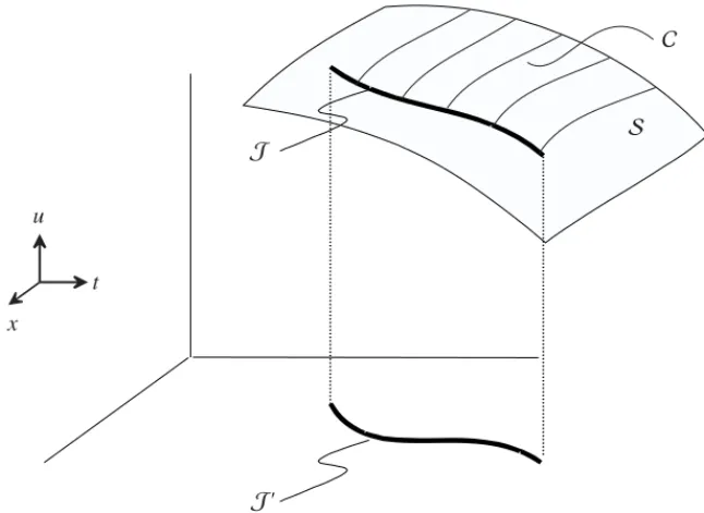
2.1 Initial curveJ and a characteristicCon the integral surfaceS. . . 14

2.2 Base characteristics of(_∗)of Example 2.2. . . 17

2.3 Region of inﬂuence and region of dependence. In the case of constant coefﬁcients these characteristics are straight lines. . . 19

3.1 Sawtooth function. . . 36

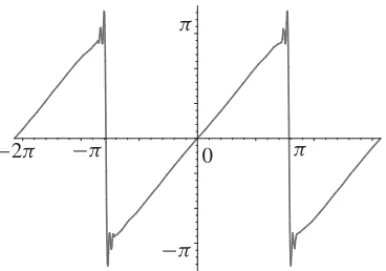
3.2 Example of Gibbs’s phenomenon (50 terms). . . 37

3.3 Aliasing. . . 44

4.1 A top hat delta sequence. . . 56

4.2 An exponential delta sequence (λ₌0.01, 0.04, 0.09, 0.25, 0.49, 1.0). . . 57

5.1 Stencil of the Laplace operator in compass notation (left) and index no-tation (right). . . 81

5.2 Stencil of the Laplace operator near a boundary. . . 82

5.3 Cylindrical (left) and spherical (right) coordinates. . . 84

5.4 Control volume for a cell-centered (left) and a vertex-centered (right) ﬁnite volume method. . . 85

5.5 Two-dimensional control volume for a cell-centered ﬁnite volume method. 87 5.6 The solution(5.84) on the intervals(0,1)(left) and(0,0.02)(right). . . . 93

5.7 Exact and numerical solutions of (5.83a) with initial conditionu(0)₌1. The numerical solution is computed with the forward Euler method with t₌1/45. . . 94

5.8 Grids for the longitudinal (left) and transversal (right) method of lines. . 96

(18)

6.1 Contact angle. . . 120

7.1 Sketch of bar element. Side view (i) and cross section (ii). . . 134

7.2 A temperature distribution. . . 139

7.3 A piece of metal heated by an electric ﬁeld. . . 140

7.4 A semi-inﬁnite bar heated fromx ₌0. . . 144

7.5 A wedge-shaped conductor heated by an electric ﬁeld. . . 146

7.6 Radial temperature distribution in wedge ofν₌ 1₂π (left) andν ₌3₂π (right) forσ A2/4κ ₌1 and 4κt /ρC ₌1₄,2₄,3₄, . . .. . . 147

7.7 A Joukowski airfoil. . . 154

8.1 The eigenvalues contained in the ﬁrst quadrant of the circlek2₊l2<_|λ_|/π. . . 168

8.2 A pointξ _∈and its mirror pointξ∗. . . 174

8.3 Asymptotic boundary condition for the velocityu. . . 181

9.1 Five-point stencil for the difference equation (9.2). . . 188

9.2 Stencil for the Robin boundary condition (9.5) without (left) and with (right) a virtual grid point W. . . 189

9.3 An unconnected grid; grid pointxCis not connected to any other grid point. . . 190

9.4 Stencil at the left boundary. . . 201

9.5 The eigenvalues ofAcompared with the exact eigenvalues forM₌20. . . 207

9.6 Lexicographic ordering of grid points forM₌4. . . 208

9.7 Convergence history of the Gauss–Jacobi and Gauss–Seidel iterative methods for the Dirichlet problem (9.40) withM₌20. . . 211

9.8 Five-point stencil for (9.115). . . 225

9.9 A patch of a staggered grid in the interior (left) and near a boundary (right). . . 225

9.10 The velocity (top) and the pressure ﬁeld (bottom) of a Stokes ﬂow in a rectangular domain. . . 227

10.1 Solution of the heat shock problem at various time levels. . . 239

10.2 Similarity coordinateγof the interface as a function of the Stefan problem parameterα. . . 247

10.3 Enthalpy functionH (T ). . . 248

10.4 Phase portrait of Fisher’s travelling-wave problem (10.71) withc₌2.25. Arrows indicate the positiveξdirection. Note the trajectory that connects saddle point(1,0)T _{with stable node}₍₀_,₀₎T_{. . . 254}

10.5 The (numerically obtained) travelling-wave solution of Fisher’s problem (10.69), (10.70) withc₌2.25 andU (0)₌1₂. . . 255

(19)

List of Figures xix

11.2 Numerical solution of the heat equation computed with the explicit Euler

scheme with time steps t ₌1.2_×10−3 _{(left) and} _t ₌₁_.₃_×₁₀−3

(right). . . 262

11.3 A solution having a sharp moving front of the heat equation with source term at three different time levels. . . 269

11.4 Stencil for the implicit scheme (11.41). . . 270

11.5 Numerical solution of the heat equation computed with the implicit Euler scheme with time steps t ₌1.2_×10−3 _{(left) and} _t =1.3_×10−3 (right). . . 272

11.6 Stencil for theϑmethod (11.49). . . 273

11.7 Numerical solution of the heat equation with discontinuous data, com-puted with theϑscheme. . . 275

11.8 Eigenvalues of the matricesB−_ϑ1 (left) andC(right) forϑ ₌0.5 (✷), 0.75(_◦), and 1(✸). . . 278

11.9 Ampliﬁcation factor ez_{compared with the rational function}_r(z)_for_ϑ = 0.5,0.75, and 1. . . 282

11.10 A two-dimensional spatial grid for initial boundary value problem (11.110) withM₌5 andN ₌4. . . 289

11.11 Patch of the grid with a moving interfacex₌S(t ). . . 299

11.12 Numerical solution of the Stefan problem (11.151). . . 302

12.1 Characteristics of the Burgers’ equation that intersect (left) or fan out (right). . . 312

12.2 The solution of (12.12) att ₌0 and 0.2 andt∗₌1/π and 0.8 for the initial conditionv(x)₌sinπ x. . . 313

12.3 Weak solution, discontinuous acrossE. . . 319

12.4 Illustration of the equal-area rule: The multivalued “solution” on the left should be replaced by the shock on the right. . . 321

12.5 Shock wave and corresponding characteristics. . . 322

12.6 Rarefaction wave and corresponding characteristics. . . 323

12.7 Characteristics corresponding to an expansion shock of the Burgers’equa-tion. . . 324

12.8 Flux function and solution of the Buckley–Leverett equation. . . 326

12.9 Illustration of the method of Massau. . . 334

12.10 Similarity solution of the Riemann problem for a 3_×3 linear system. The triple(β1, α2, α3)denotes the solutionu=β1s1+α2s2+α3s3, etc. 338 12.11 Wave pattern of ak-simple wave. . . 339

12.12 Wave pattern of a contact discontinuity. . . 340

12.13 Wave pattern of ak-shock. . . 341

12.14 Possible wave patterns of the Riemann problem for the shallow-water equations. . . 343

12.15 The 1-wave is either a shock (left) or a rarefaction wave (right). . . 344

12.16 The functiong(z). . . 345

12.17 The 2-wave is either a shock (left) or a rarefaction wave (right). . . 346

(20)

13.1 Stencil for the upwind scheme. The dotted line is the characteristic

through the point(xj, tn+1)facing back to the initial linet=0. . . 365

13.2 Numerical approximation of a sine wave computed with the upwind scheme. . . 367

13.3 Stencil for the Lax–Wendroff scheme. The dotted line is the characteristic through the point(xj, tn+1)facing back to the initial linet=0. . . 368

13.4 Numerical approximation of a sine wave computed with the Lax–Wendroff scheme. . . 370

13.5 Amplitude and phase errors of the upwind scheme (left) and the Lax– Wendroff scheme (right). . . 372

13.6 Numerical solution computed with the upwind scheme (left) and the Lax– Wendroff scheme (right), after 25, 50, and 75 time steps, respectively. . . 374

13.7 Numerical solution of the advection-diffusion equation computed with the central difference scheme. . . 376

13.8 Numerical solution of the advection-diffusion equation computed with the upwind scheme. . . 378

13.9 Stencil for the box scheme. The open circles indicate the intermediate grid points. . . 380

13.10 Phase error of the box scheme. . . 381

13.11 Numerical sine wave (left) and step function (right) computed with the box scheme. . . 382

13.12 Stencil for the leapfrog scheme. . . 382

13.13 Relative phase error of the leapfrog scheme. . . 384

13.14 Numerical group velocity of the box scheme. . . 385

13.15 The effect of the numerical group velocity on a wave packet computed with the box scheme. . . 386

13.16 Piecewise constant numerical solution at time leveltn_{. . . 387}

13.17 Ashock wave solution of the Burgers’equation computed with Godunov’s scheme (left) and the upwind scheme (right). . . 391

13.18 The van Leer, superbee, and minmod limiters in the TVD region. . . 400

13.19 Piecewise linear numerical solution at time leveltn. . . 403

13.20 Numerical solution computed with the slope limiter method, after 25, 50, and 75 time steps, respectively. . . 406

13.21 Rarefaction wave computed with the slope limiter method. . . 408

13.22 Numerical solution of the leapfrog scheme, corrupted by the erroneous boundary conditionu(1, t )₌0. . . 409

13.23 Eigenvalues of the leapfrog scheme with upwind numerical boundary condition. . . 413

14.1 Schematic representation of a similarity solution in the(x, t )plane. . . . 427

14.2 Numerical approximation of the dam break problem at time levels 0.5 (top) and 1.0 (bottom). . . 436

14.3 Schematic representation of a critical 1-rarefaction wave for the shallow-water equations. . . 439

14.4 Stencil for the centred scheme (14.102b). . . 441

(21)

List of Figures xxi

14.6 TheC₂characteristic through the boundary grid point(xM+1, tn+1). . . . 448

14.7 Numerical approximation of the geopotentialϕ ₌ghat time levels 0.3,0.4, . . . ,0.8. . . 450

14.8 Two time levels in the staggered grid for the leapfrog scheme. The vari-ablesuandrare deﬁned at points marked by_•and_◦, respectively. . . . 454

15.1 A plot ofx₊sin(εx)₊e−x/ε_{and its nonuniform asymptotic} approxima-tionx₊εxforε₌0.01. . . 462

15.2 Analysis of distinguished limits. . . 465

15.3 Slowly varying bar. . . 469

15.4 Plots of the approximate solution and a numerically “exact” solution y(t_;ε)of the air-damped resonator problem forε₌0.1. . . 489

16.1 Schematic representation of a three-layer panel. . . 501

16.2 The reaction ratekas a function of the temperatureT. . . 503

16.3 Temperature and concentration distribution in a symmetrically heated panel. . . 506

16.4 Temperature and concentration at the centre of a symmetrically heated panel. . . 507

16.5 Pattern formation in glass by masked erosion (courtesy P.J. Slikkerveer, Philips Research Laboratories, Eindhoven). . . 509

16.6 Cross section of a hole in the substrate. . . 509

16.7 Characteristics and shocks of a two-dimensional trench forδ₌0.1 and k₌2. . . 513

16.8 Solution for the surface position (left) and its slope (right) of a one-dimensional trench. Parameter values areδ₌0.1 andk₌2.33. . . 515

16.9 Analytical solution (left) and measurements (right) of the surface position for a two-dimensional trench att ₌0.5, 1.1, 1.6, and 2.1 (experimental results by P.J. Slikkerveer [155]). . . 516

16.10 Temperature and concentration distribution in a reactor vessel. . . 522

16.11 Temperature and concentration at the centre of a reactor vessel. . . 523

16.12 Viscoelastic material suddenly compressed. . . 524

16.13 uz,trr, andtzz atz=L, z=0.9L,z=0.6L, and z=0, plotted as a function of time. At the left side are the results in the boundary layer, while at the right side are the results for larger time. . . 530

16.14 Impression of a suspended cable consisting of three interconnected spans. 532 16.15 Sketch of cable element stretched under tension. . . 532

16.16 Sketch of cables connected at a suspension string. . . 533

16.17 An oscillating cable section (from top to bottom): the vertical displace-ment dY insLfor various time steps, the position at the middle (s₌ 1₂) of the displacement in time, and the varying part of the tension dT in time. All variables are dimensional. . . 539

16.18 Sketch of groundwater and rain problem. . . 541

16.19 Plot of boundary layer proﬁleψ0(ξ )forK=O(1). . . 543

16.20 Sketch of a silicon bar. . . 547

(22)

16.22 Temperature distribution in the monocrystalline bar. . . 554 16.23 A spherical catalyzer pellet. . . 556 16.24 r1as a function of 1/λ. . . 560

16.25 Leading-order approximation forα_→0 andλ₌O(1). . . 561

16.26 Acoustic refraction in shear ﬂow. . . 563 16.27 A ray tube. . . 568 16.28 A ray tube starting from a circle of radiusεin theY Zplane, refracting

downward in right-running shear ﬂow. . . 569 16.29 Mass conservation between streamlines. . . 575 16.30 Inclined plane surface. . . 576 16.31 Streamlines along a ﬂat plate. . . 577 16.32 Inclined cylinder. . . 578 16.33 Streamlines along an inclined cylinder issuing from a point source in the

wall. Right: analytical solution; left: experiments by one of the authors (SWR). Note the realistic but (strictly speaking) not modeled crossing streamlines! . . . 580 16.34 Sketch of conﬁguration. Rp=Rp(z−zp)is the plunger surface,Rm=

Rm(z)is the mould surface,zp(t )is the position of the plunger top, and

b(t )is the position of the glass surface. . . 583 16.35 Sketch of the control surfaces to calculate the axial ﬂux. . . 587 16.36 Dimensionless position (left) and minus pressure gradient (right)

corre-sponding to a plunger entering a mould fully ﬁlled with ﬂuid glass. . . . 588 16.37 The three events in a laser percussion drilling process where a melting

model is needed: (a) melting, (b) splashing, and (c) resolidiﬁcation. . . . 590 16.38 The geometry of the laser-induced melting problem. . . 592 16.39 The position of the solid-liquid interface for the case of aluminium. The

absorption of latent heat is neglected. . . 594 16.40 Relation between enthalpy and temperature for pure crystalline

sub-stances and for glassy subsub-stances and alloys. . . 595 16.41 Time history plots for temperature at the interface in the

enthalpy problem. . . 597 16.42 Time development of concentration of methyl-hippuric and mandelic acid

after (from left to right) 1, 3, and 5 s of migration. . . 603 16.43 Distribution of local pH (lower trace) and local electric ﬁeld (upper trace)

once the steady state is reached. . . 604 16.44 Migration of mandelic acid from steady state with 2, 5, 10, and 20 s of

diffusion (overlapping proﬁles on the left) and after restoration of the driving current in six 200 ms intervals. . . 604 16.45 A schematic picture of the Stirling-type pulse tube refrigerator: (a) the

(23)

List of Figures xxiii

(24)

(25)

List of Tables

12.1 Number of boundary conditions for the shallow-water equations. . . 358

14.1 Conditions for shocks and rarefaction waves. . . 434

16.1 Parameters involved in the curing process. . . 503

16.2 Parameters for a thermal explosion. . . 518 16.3 Typical parameter values of silicon. . . 548

16.4 Typical values of the parison problem parameters. . . 584

16.5 Parameters for the laser drilling process applied to aluminium using an

Nd:YAG-laser. . . 591

16.6 Component data in the simulation. The mobilities are in

10−9_m2_/(_V_·_s₎_{and the diffusion coefﬁcients are in 10}−9_m2_/_{s. . . 602}

16.7 Physical data for a typical single-inlet pulse tube (values at 300 K). . . . 611

D.1 Coefﬁcients for the BDF. . . 633

D.2 Coefﬁcients for the Adams–Bashforth formula. . . 634

D.3 Coefﬁcients for the Adams–Moulton formula. . . 634

(26)

(27)

Notation

Variables and Operators

t time

x space coordinate inR

x₌(x, y)T,x₌(x, y, z)T space coordinate inRd(d ₌2,3)

v(x, t ), v(x, t ) scalar function

v(x, t ),v(x, t ) vector function

(u, v) inner product of the scalar functionsuandv

u·v inner product of the vectorsuandv

u×v vector product of the vectorsuandv

L(x, t )_[v_] differential operatorL(x, t )applied tov

L∗₍_x_{, t )} _{adjoint operator of}_L(_x_{, t )}

dv

dx, v′ derivative ofv(x)

∂v

∂x, vx partial derivative ofv(x, t )

∂v

∂n,n·∇v directional derivative ofvin the direction ofn

∇v gradient ofv

∇·v divergence ofv

∇×v curl ofv

∇2v Laplace operator applied tov

vdV generic integral over a domain⊂R

d_(d =2,3)

v(x, t )dxdy integral over a domain⊂R

2

∂v·ndS integral over a closed surface∂⊂R

3

Cv·dℓ integral over a closed contourC⊂R

d_(d =2,3)

[v_]+₋ jump ofvacross a discontinuity

ex,ey,ez unit vectors in the Cartesian coordinate system(x, y, z)

er,eφ,ez unit vectors in the cylindrical coordinate system(r, φ, z)

er,eθ,eφ unit vectors in the spherical coordinate system(r, θ, φ)

(28)

Numerical Parameters and Variables

t step size

x grid size inxdirection

h generic grid size

xj jth grid point

xj₊1/2 location of a control volume boundary

tn _{time level}_nt

v_jn numerical approximation ofv(x, t )

at grid pointxj and time leveltn

F_jn₊₁_/₂ numerical approximation of ﬂuxf (x, t )

at control volume boundaryxj+1/2and time

leveltn

C, E, etc. location names of grid points

xC generic grid point

vC numerical approximation ofv(xC)

v grid function

L[vjn] difference operatorLapplied tovjn

L−1

inverse ofL

dn

j =O(x

2₎ _dn

j is of the orderx

2_for_x _→₀

Vectors and Matrices

v₌(v1, v2, . . . , vn)T column vector inRn vT ₌(v1, v2, . . . , vn) row vector inRn

vk _k_{th vector in a sequence}

v p p-norm ofv

A₌(aij) matrix withaij inith row andjth column

A₌(a1,a2, . . . ,an) matrix withaias theith column

AT _{the transpose of}_A

A−1 the inverse ofA

I identity matrix

diag(a1, a2, . . . , an) diagonal matrix withaiinith row and column

detA determinant ofA

A p p-norm ofA

(29)

Notation xxix

Miscellaneous

:=, _=: is deﬁned as, deﬁnes

.

= is equal to when neglecting terms of higher order

∼ is asymptotically equal to

O asymptotic order symbol (“bigO”)

o asymptotic order symbol (“smallo”)

e base of the natural logarithm(e₌2.71828. . .)

i imaginary unit

|z_| absolute value or modulus ofz_∈C

z complex conjugate ofz_∈C

[v_] dimension of variable/constantv(e.g., in SI units)

C characteristic/curve inRd_(d

=2,3)

(30)

(31)

Preface

There exist a number of good textbooks on both the analytical and the numerical aspects of PDEs. So why another book on PDEs, then? Well, most existing texts deal with either analytical or numerical aspects, but not both. There are understandable reasons for this. For one thing, it is the traditional approach. The impressive achievements in understanding a large variety of physical phenomena, long before computers came into use, have made the study of PDEs, often called applied mathematics, a well-established area in its own right, which will no doubt remain so for many years to come. At the same time, although this area has grown impressively, it has become clear that nowadays the power of this branch of mathematics does not so much lie in constructive solutions but rather in giving qualitative answers, thus having a usefulness in its own right. Notwithstanding the achievements it has brought by answering some deep questions such as those regarding existence and uniqueness, and by developing a host of instruments to grasp the solution, its machinery for concretely solving problems is still limited to simplified geometries and the use of expansions in terms of special functions and the like. Yet often the actual solution is the ultimate goal of the scientist or engineer who needs concrete answers. The advent of fast computers and the equally fast development of numerical methods filled this gap to a large extent, so that modern engineers can use a large variety of packages to find numerical approximations to the solutions of their problems. This is reflected in the literature on numerical books. In fact, the latter subject has grown to such an extent that different approaches, like finite elements and finite differences, often appear to be as far apart from each other as they are from a purely analytical text. But despite the importance of standard software, problems are more often than not standard and a thorough knowledge of at least a well-chosen subset of analytical and numerical tools and methodologies is necessary when dealing with real-life problems.

Only when dealing with PDEs in practice does it become clear that numerical treatment and analytical treatment of the subject are both needed. A numerical analyst devoted to computing a Dirichlet problem on a square by yet another method is as esoteric as an applied mathematician who is trying to see the world as built up by spheres and cylinders. This gives the main motivation for this text. We are deeply convinced that we need to treat PDEs by combining analytical and numerical aspects. The two supplement each other but have, conceptually, much in common, too. Nevertheless, concepts and theoretical problems, however sophisticated, are not enough to teach us how to deal with PDEs in practice. In a practical situation one is supposed to make a mathematical model first, obtain insights into the behaviour of the solution, and finally compute the solution (or sometimes be satisfied with a qualitative understanding of the problem). Hence, as a third component, insight into

(32)

modeling real-life problems needs to complement and deepen theoretical and numerical knowledge.

This book, therefore, intends to address three aspects: the analysis of PDEs (including some basic knowledge of tools), numerical solution methods, and, last but not least, model-ing. In a way, the analytical part follows some of the classical lines. As for numerics, we had to make a choice. Most numerical books focus on either finite difference methods or finite element methods (FEMs). This has a simple explanation: the setting is so large that some choices have to be made. The FEM is quite versatile with respect to the domains on which a problem can be defined. Therefore it is most appropriate for boundary value problems. It requires, however, quite a bit of preparatory work, so that a textbook with these ideals would become too big to handle. We wanted to provide a general introduction to solving PDEs numerically, and for this purpose finite differences (and finite volumes, where they come in handy as well) are sufficiently general. Their introduction is straightforward, as is their use. Moreover, given the insights gained from this text, it should not be hard to use FEMs at proper places instead. Another choice we made deals with the number of nonlinear problems one can treat. Due to lack of space (and also because of didactical constraints), we deal with nonlinearities mostly in a generic way, but certainly do not avoid them. As for the modeling part, we believe that dimensional analysis is an obligatory ingredient. Moreover, modeling can only be learned by doing, so we need a larger number of case examples. We have therefore included a separate chapter, with problems from practice, all from the personal experience of the authors.

(33)

Preface xxxiii

variation and method of strained coordinates) and two of which are of singular perturbation type (method of matched asymptotic expansions and method of multiple scales, including rays). It is shown how often remarkably sharp analytic approximations to solutions can be obtained while revealing a lot of the problem’s structure. This plays an important role in actual modeling, as explicit parametric dependence clearly gives more insight than numbers often do. The last chapter, Chapter 16, contains a large number of case studies. Here a true amalgamation of all previous theories and techniques takes place. It can be used alongside other relevant chapters, where references to this chapter enable the user to work out a related practical problem. The various sections in Chapter 16 also give many suggestions for further modeling, which could typically be used in a course with room for larger projects.

The computations for this book were done using MATLAB®. There exists a host of packages and toolboxes to solve PDEs numerically. We have tried to avoid exercises for which elaborate computer usage would be required. A course taught from this book will beneﬁt, however, from assignments dealing with some larger problems, including (less trivial) numerical computations. The exercises at the end of each chapter and in particular the case studies in Chapter 16 should give ideas for this.

The book is intended for use in courses at an advanced undergraduate or a graduate level. It has been designed so that it should be useful both for engineers, who may be more interested in the methods as such, and for more mathematically interested readers. To this end, we have made it self-contained. Teachers may judge for themselves which parts they deem more relevant, given the needs or interests of their audience. By including an extensive index and ample cross-referencing, we hope that this book is also quite suitable for self-study and for reference. The authors have had positive experiences with courses taught from the material of this book. Over the years we have beneﬁted a great deal from the suggestions and remarks of many colleagues, and of course of our students. We owe them a debt, as we will owe to those readers who will share with us their experiences and recommendations. We would like to gratefully acknowledge, nevertheless, the advice of a few people in particular: A.E. Dahoe, J. de Graaf, R. Horvath, I. Lyulina, B. O’Malley, J. Molenaar, V. Nefedov, N.C. Ovenden, M. Patricio, N. Peake, J. Rijenga, W.H.A. Schilders, P.J. Slikkerveer, W.R. Smith, A.A.F. van de Ven, and K. Verhoeven.

We are indebted to the staff of SIAM for their help and patience with this project, which took us much longer to complete than originally anticipated.

(34)

(35)

Chapter 1 Differential and Difference

Equations

In this chapter we give a brief introduction to PDEs. In Section 1.1 some simple prob-lems that arise in real-life phenomena are derived. (A more detailed derivation of such problems will follow in later chapters.) We show by a number of examples how they may often be seen as continuous analogues of discrete formulations (i.e., based on difference equations). In Section 1.2 we brieﬂy summarize the terminology used to describe various PDEs. Thus concepts like order and linearity are introduced. In Chapter 2 we shall dis-cuss the classiﬁcation of the various types of PDEs in more detail. Finally, we introduce difference equations and notions like scheme and stencil, which play a role in numerical approximation, in Section 1.3.

1.1 Introduction

Many phenomena in nature may be described mathematically by functions of a small number of independent variables and parameters. In particular, if such a phenomenon is given by a function of spatial position and time, its description gives rise to a wealth of (mathematical) models, which often result in equations, usually containing a large variety of derivatives with respect to these variables. Apart from the spatial variable(s), which are essential for the problems to be considered, the time variable will play a special role. Indeed, many events exhibit gradual or rapid changes as time proceeds. They are said to have anevolutionary character and an essential part of their modeling is therefore based oncausality; i.e., the situation at any time is dependent on the past. As far as (mathematical) modeling leads to PDEs, the latter will be called evolutionary, i.e., involve the timet as a variable. The other type of problems are often referred to assteady state. We will give some examples to illustrate this background.

A typical PDE arises if one studies the ﬂow of quantities like density, concentration, heat, etc. If there are no restoring forces, they usually have a tendency to spread out. In particular, one may, e.g., think of particles with higher velocities (or rather energy) colliding with particles with lower velocities. The former are initially rather clustered. The energy will gradually spread out, mainly because the high-velocity particles collide with other ones, thereby transferring some of the energy. This is calleddissipation. A similar effect can be

(36)

observed for a material dissolved in a ﬂuid with concentrations varying in space. Brownian motion will gradually spread out the material over the entire domain. This is calleddiffusion.

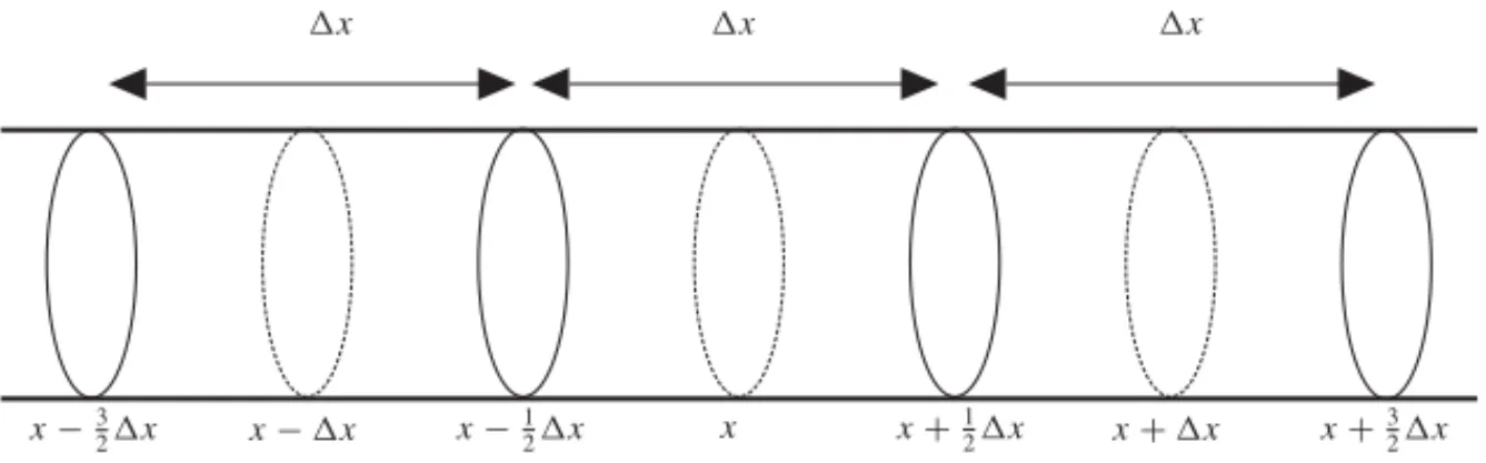
Example 1.1 Consider a long tube of cross sectionAﬁlled with water and a dye. Initially the

dye is concentrated in the middle. Letu(x, t )denote the concentration or density (mass per unit length) of the dye at positionxand timet; then we see that in a small volumeAx, positioned betweenx− 12xandx+

1

2x(Figure 1.1), the total amount of dye equals approximately u(x, t )x. Now consider a similar neighbouring volumeAx betweenx+ 12xandx+ 3

2x, with a corresponding dye concentrationu(x+x, t ). The mass that flows per unit time through a cross section is called the mass flux. From the physics of solutions it is known that the dye will move from the volume with higher concentration to one with lower concentration such that the mass fluxf between the respective volumes is proportional to the difference in concentration between both volumes and is thus given by

f

x+1₂x, t

=α

u

x+1₂x, t

_u(x

+x, t )₋u(x, t ) x ,

whereα, the diffusion coefﬁcient, usually depends onu. This relation is called Fick’s law for mass transport by diffusion, which is the analogue of Fourier’s law for heat transport by conduction.

As there is a similar ﬂux between the centre volume and its left neighbour, we have a rate of change of total amount of mass in the centre volume equal to the difference between both ﬂuxes given by

∂

∂tu(x, t )x=f

x+1₂x, t

−f

x−1₂x, t

.

If the diffusion coefﬁcientαis a constant, we have

∂

∂tu(x, t )=α

u(x+x, t )−2u(x, t )+u(x−x, t )

x2 . (∗) By taking the limits for small volumes (i.e.,x_→0), we ﬁnd

∂

∂tu(x, t )=α ∂2 ∂x2u(x, t ),

which is called the one-dimensionaldiffusion equation. As heat conduction satisﬁes the same equation, it is also called theheat equationifudenotes temperature. ✷

x−3

2x x−x x− 1

2x x x+

1

2x x+x x+ 3 2x

x x

x

(37)

1.1. Introduction 3

Another kind of PDE occurs in the transport of particles. Here a ﬂow typically has a dominant direction; mutual collision of particles (which is felt globally as a kind of internal friction, or viscosity) is neglected.

Example 1.2 Consider a road with heavy trafﬁc moving in one direction, say thexdirection

(Figure 1.2). Let the number of cars at timeton a stretch[x, x+x]be denoted byN (x, t ). Furthermore, let the number of cars passing a pointxper time periodtbe given byf (x, t )t. In that period the number of carsN (x, t₊t )can only be changed by a difference between inﬂow atxand outﬂow atx+x; i.e.,

N (x, t₊t )₌N (x, t )₋f (x₊x, t )₋f (x, t )t.

Rather than the number of carsNper interval of lengthx, it is convenient to consider acar densityn(x, t ), which is deﬁned by

N (x, t )=n(x, t )x. Hence we obtain the relation

n(x, t₊t )₋n(x, t ) t = −

f (x₊x, t )₋f (x, t ) x .

Assuming sufﬁcient smoothness (which implies that we have to allow for fractions of cars. . .), this leads in the limit oft, x→0 to

∂n ∂t +

∂f ∂x =0,

which takes the form of aconservation law. We may recognizef again as a flux. If this flux only depends on the local car density, i.e.,f =f (n), andf is sufficiently smooth, we obtain

∂n ∂t +f

′_(n)∂n ∂x =0,

also known as thetransport equation. ✷

x _x₊_x

Figure 1.2.Sketch of trafﬁc ﬂow.

An important class of problems arises from classical mechanics, i.e., Newtonian sys-tems.

Example 1.3 Consider a chain consisting of elements, each with massm, and springs, with

spring constantβ >0 and lengthx; see Figure 1.3. Denote the elements byV1, V2, . . . with position of the massesx=u1, u2, . . .. Assuming linear springs, the force necessary to increase the original lengthxof the spring of elementViby an amountδi=ui−ui−1−xis equal toFi=βδi. Apart from the endpoints, all masses are free to move in thexdirection, their

inertia being balanced by the reaction forces of the springs. Noting that each elementVi(except

for the endpoints) experiences a spring force from the neighbouringith and(i+1)th springs, we have from Newton’s law for theith element that

md 2_u

i

(38)

V1 V2

u1 u2

Δ_x ␦

i

ui–1 ui

Figure 1.3.Chain of coupled springs.

If the chain elements increase in number, while the springs and masses decrease in size, it is natural and indeed more convenient not to distinguish the individual elements, but to blend the discrete description of (_∗) into a continuous analogue. The small masses are conveniently described by a densityρsuch thatm=ρx, while the large spring constants are best described by a stiffnessσ₌βx. Then we obtain from (_∗) for the position functionu(x, t )the PDE

∂2u ∂t2 =

σ ρ

∂2u

∂x2. (†)

As solutions of this equation are typically wave like, it is known as thewave equation, with a wave velocity equal to√σ/ρ. In our example it describes longitudinal waves along the suspended chain of masses. In the context of pressure-density perturbations of a compressible ﬂuid like air, the equation describes one-dimensional sound waves, e.g., as they occur in organ pipes. In that case the air stiffness is equal toσ ₌γp, whereγ ₌1.4 is a gas constant andp is the atmospheric pressure (see Section 6.8.2). ✷

In the following example we mention the analogue in electrical circuits of the motion of coupled spring-dashpot elements.

Example 1.4 The time-behaviour of electric currents in a network may be described by the

variables potentialV, currentI, and chargeQ. If the network is made of simple wires connecting isolated nodes, resistances, capacities, and coils, and the frequencies are low, it may be modeled (a posteriori conﬁrmed by analysis of the Maxwell equations) one dimensionally by a series of elements with the material properties resistanceR, capacitanceC, and inductanceL. Such a model is called an electrical circuit. If the frequencies are high, such that the wavelength is comparable with the length of the conductors, we have to be more precise. As the signal cannot change instantaneously at all locations, it propagates as a wave of voltage and current along the line. In such a case we cannot neglect the resistance and inductance properties of the wires. By considering the wires as being built up from a series of (inﬁnitesimally) small elements, we can model the system by what is called a transmission line, leading to PDEs in time and space.

(39)

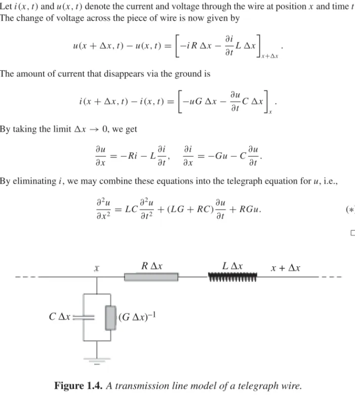
1.1. Introduction 5

A famous example is thetelegraph equation, where an inﬁnitesimal piece of telegraph wire is modeled (Figure 1.4) as an electrical circuit consisting of a resistanceRxand an inductance Lx, while it is connected to the ground via a resistance(Gx)−1_{and a capacitance}_Cx_. Leti(x, t )andu(x, t )denote the current and voltage through the wire at positionxand timet. The change of voltage across the piece of wire is now given by

u(x₊x, t )₋u(x, t )₌ ₋iR x₋∂i ∂tL x

x+x .

The amount of current that disappears via the ground is

i(x+x, t )−i(x, t )= −uG x−∂u ∂tC x

x .

By taking the limitx→0, we get

∂u

∂x = −Ri−L ∂i ∂t,

∂i

∂x = −Gu−C ∂u

∂t.

By eliminatingi, we may combine these equations into the telegraph equation foru, i.e.,

∂2u ∂x2 =LC

∂2u

∂t2 +(LG+RC) ∂u

∂t +RGu. (∗)

✷

CΔ_x

RΔx LΔx _{x +}Δ_x

(GΔx)–1

Figure 1.4.A transmission line model of a telegraph wire.

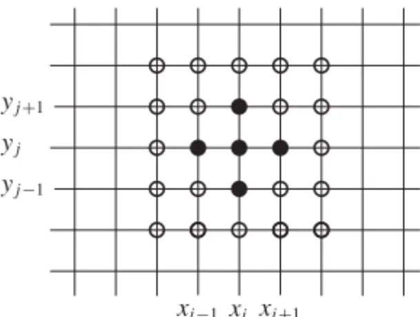
Example 1.5 Consider the following crowd ofN2very accommodating people (Figure 1.5),

for convenience ordered in a square of sizeL_×L, while each person, labelled by(i, j ), is positioned atxi=ih, yj=j h, withh=L/N. Each person has an opinion given by the

(scalar) numberpijand can only communicate with his or her immediate neighbours. Assume

that each person tries to minimize any conﬂict with his or her neighbours and is willing to take an opinion that is the average of their opinions. So we have

pij =

1 4

(40)

xi xi+1 xi−1 yj

yj−1 yj+1

Figure 1.5.An array of accommodating individuals.

If the number of people becomes so large that we may take the limitN→ ∞(i.e.,h→0) and pbecomes a continuous function of(x, y), (∗) becomes

p(x, y)= 1

4(p(x+h, y)+p(x−h, y)+p(x, y+h)+p(x, y−h)). This may be recast into

p(x+h, y)−2p(x, y)+p(x−h, y)+p(x, y+h)−2p(x, y)+p(x, y−h)=0. If this is true for anyh, we may divide byh2, and the equation becomes in the limit

∂2p ∂x2 +

∂2p ∂y2 =0.

This equation is called theLaplace equationand describes phenomena where, in some sense, information is exchanged in all directions until equilibrium is achieved. From the above sociological example it is not difﬁcult to appreciate that discontinuities and sharp gradients are smoothed out, while extremes only occur at the boundary. The best-known problem de-scribed by this equation is the stationary distribution of the temperature in a heat-conducting

medium. ✷

1.2 Nomenclature

In the previous section we met a number of equations with derivatives with respect to more than one variable. In general, such equations are calledpartial differential equations. Letx

andtbe two independent variables and letu(x, t )denote a quantity depending onxand t.

Furthermore, let

t _{∈ [}0, T_], 0_≤T _{≤ ∞}, x_{∈ [}a, b_{] ⊂}R. (1.1)

For an integerna general form for a scalar PDE (in two independent variables) reads

F

∂nu ∂tn ,

∂nu ∂t ∂xn−1, . . . ,

∂nu ∂xn,

∂n−1u ∂tn−1, . . . ,

∂n−1u ∂xn−1, . . . ,

∂u ∂t,

∂u ∂x, u, x, t

=0. (1.2)

The highest-order derivative is called the order of the PDE; not all partial derivatives

(41)

1.2. Nomenclature 7

implicit formulation, i.e., the highest-order derivative(s), the principal part, do(es) not

appear explicitly. If the latter is the case, we call it anexplicitPDE. The generalization to more than two independent variables is obvious.

Example 1.6 Some important examples of PDEs are as follows:

(i) ∂u ∂t +c

1+3₂u

∂u ∂x +

1 6ch

2∂3u

∂x3 =0 (Korteweg–de Vries equation). This is a third order PDE.

(ii) ∂u ∂t +

∂

∂xf (u)=0 (nonlinear transport equation). Iff is differentiable, we see that this is a ﬁrst order PDE inu.

(iii) ∂u ∂t +u

∂u ∂x =ε

∂2u

∂x2 (the Burgers’ equation).

Ifε₌0, this may be referred to as the inviscid Burgers’ equation, which is a special case of the transport equation.

(iv) ∂ 2_u ∂t2 −c

2∂2u ∂x2 −

1 3h

2 ∂4u

∂x2_∂t2 =0 (linearized Boussinesq equation). (v) EI∂

4_u ∂x4 −T

∂2u ∂x2 +m

∂2u

∂t2 =0 (vibrating beam equation). (vi) ∂u

∂y ∂2u ∂y∂x −

∂u ∂x

∂2u ∂y2 =ν

∂3u

∂y3 (Prandtl’s boundary layer equation). ✷

In quite a few cases the order can only be deduced after some (trivial) manipulation.

Example 1.7 ∂u ∂t − ∂ ∂x D(u)∂u ∂x

=f (x) (nonlinear diffusion equation).

It is clear that this PDE is second order. There is no analytical, numerical, or practical need to rework this and have ∂2

∂x2uappear explicitly. ✷ Usually, the variables are space and/or time. Although the variables in (1.2) are generic, we shall use the symbolt to indicate thetimevariable in general. The variable

xwill refer tospace. There are major differences between problems where time does and does not play a role. If the time is not explicitly there, the problem is referred to as a

steady state problem. If the PDE possesses solutions that evolve explicitly witht, we call it an evolutionary problem; i.e., there is causality. Most of the theory will be devoted to problems in one space variable. However, occasionally we shall encounter more than one such space variable. Fortunately, problems in more such variables often have many analogues of the one-dimensional case. We shall indicate vectors by boldface characters. So in higher-dimensional space the space variable is denoted byx, or by(x, y, z)T. The PDE can still be scalar. We have obvious analogues for vector-dependent variables of the foregoing.

Example 1.8 A few other examples are as follows:

(i) ∂u ∂t −α

∂2u ∂x2 +

∂2u ∂y2 +

∂2u ∂z2

(42)

We prefer to write this as ∂ ∂tu−α∇

2

u=0.∇2is referred to as theLaplace operator.

(ii) ∂ 2_u ∂t2 −c

2

∇2u₌0 (wave equationin three dimensions). (iii) _∇2

u+k2u=0 (Helmholtz or reduced wave equation). (iv) (1₋M2)∂

2_u ∂x2 +

∂2u ∂y2 +

∂2u

∂z2 =0 (equation for small perturbations in steady sub-sonic (M2<1) or supersonic (M2>1) ﬂow). ✷

Sometimes one also denotes a partial derivative of a certain variable by an index:

ut:= ∂u

∂t, ut x:= ∂2u

∂t ∂x. (1.3)

If we can write (1.2) as a linear combination ofuand its derivatives with respect toxand

t, and with coefﬁcients only depending onxandt, the PDE is calledlinear. Moreover, it is calledhomogeneousif it does not depend explicitly onx and/ort. If the PDE is a linear combination of derivatives but the coefﬁcients of the highest derivative, sayn, depend on

(n₋1)th order derivatives at most, then we call itquasi-linear[29].

For any differential equation we have to prescribe certain initial conditions and bound-ary conditions for the time and space variable(s), respectively. In evolutionbound-ary problems they often both appear as initial boundary conditions. We shall encounter various types and combinations in later chapters.

We ﬁnally remark that we may look for solutions that satisfy the PDE in a weak sense. In particular, the derivatives may not exist everywhere on the domain of interest. Again we refer to later chapters for further details.

1.3 Difference Equations

Initially, the actual form of the equations we derived in the examples in Section 1.1 was of a difference equation. Like a PDE, we may define a partial difference equation as any relation between values ofu(x, t )where(x, t )_∈F _{⊂ [}a, b_{] × [}0, T ),Fbeing a finite set of points of the domain[a, b_{] × [}0, T ). We shall encounter difference equations when solving a PDE numerically, so they should approximate the PDE in some well-defined way. The simplest way to describe the latter is by defining ascheme, i.e., a discrete analogue of the (continuous) PDE. Since we shall mainly deal with finite difference approximations in this book, we perceive a scheme as the result of replacing the differentials by finite differences. To this end we have to indicate some (generic) points in the domain_[a, b_{] × [}0, T )at which

the function valuesu(x, t )are taken. The latter set of points is called astencil. We shall

clarify this with some examples.

Example 1.9

(i) Consider Example 1.1 again. If we replace ∂

∂tu(x, t )in equation (∗) by a straightforward

discretisation, then we obtain the scheme

u(x, t+t )−u(x, t ) t =α

(43)

1.3. Difference Equations 9

t t₊t

x₋x x x₊x

Figure 1.6. Stencil of Example1.9(i).

(ii) Consider the wave equation (†) of Example 1.3. A discrete version may be found to be

u(x, t+t )−2u(x, t )+u(x, t−t ) t2

= σ ρ

u(x+x, t )−2u(x, t )+u(x−x, t ) x2 . The stencil is given in Figure 1.7. ✷

t₋t t t₊t

x₋x x x₊x

Figure 1.7. Stencil of Example1.9(ii).

Given the special role of time and the implication it has for the actual computation, which should be based on the causality of the problem, we may distinguish schemes ac-cording to the number of time levels involved. If(k₊1)such time levels are involved, we

call the scheme ak-step scheme. If the scheme involves only spatial differences at earlier time levels, it is calledexplicit; otherwise it is calledimplicit.

Example 1.10

(i) The schemes in Example 1.9 are both explicit, the ﬁrst being a one-step and the second a two-step scheme.

(ii) We could also approximate theuxxterm in the heat equation at time levelt+tand

obtain the scheme

u(x, t+t )−u(x, t ) t

(44)

This scheme has the stencil given in Figure 1.8. Clearly, it is an implicit one-step

scheme. ✷

t t₊t

x₋x x x₊x

Figure 1.8. Stencil of Example1.10(ii).

1.4 Discussion

• The use of the variablesxandy in an equation does not mean that the PDE cannot

have an evolutionary character. There are some cases where they refer to spatial coordinates, yet the corresponding equation may be hyperbolic, a type of equation we will encounter in the next chapter as an instance of evolutionary type.

• If in a system of time-dependent PDEs all spatial derivatives are replaced by suit-able difference approximations, we obtain a system of ODEs in time. If one of the PDEs is independent of time, we obtain adifferential-algebraic system. A typical example is the condition that an incompressible ﬂow is divergence free (equivalent to conservation of mass), as in the Stokes equations. This problem will be discussed in Section 8.7.