*e-mail: [email protected]
Simulation of the Solidification of Pure Nickel Via the Phase-field Method
Alexandre Furtado Ferreira*, Alexandre José da Silva, José Adilson de Castro
Program in Metallurgical Engineering, Universidade Federal Fluminense – UFF/EEIMVR,
Av. dos Trabalhadores, n. 420, 27255-125 Volta Redonda - RJ, Brazil
Received: April 25, 2005; Revised: November 30, 2006
The Phase-Field method was applied to simulate the solidification of pure nickel dendrites and the results compared with those predicted by the solidification theory and with experimental data reported in the literature. The model’s behavior was tested with respect to some initial and boundary conditions. For an initial condition without supercooling, the smooth interface of the solid phase nucleated at the edges of the domain grew uniformly into the liquid region, without branching. In an initially supercooled melt, the interface became unstable under 260 K supercooling, generating ramifications into the liquid region. The phase-field results for dendrite tip velocity were close to experimental results reported in the literature for supercooling above 50 K, but they failed to describe correctly the nonlinear behavior predicted by the collision-limited growth theory and confirmed by experimental data for low supercooling levels.
Keywords: solidification, phase-field, mathematical modeling, nickel
1. Introduction
Understanding dendritic solidification is highly important because the microstructural scales of the dendrite determine the proprieties of the material. Although significant advances have been achieved in understanding dendritic structures in past decades, our knowledge concerning dendritic growth phenomena is largely based on experi-ments and idealized theoretical models.
The first well-known paper about the Phase-field Method, pro-posed by Caginalp1, dates back to 1980. Since then, the method has proved to be suitable for describing the complex growth of the unstable solid/liquid interface during solidification phenomena. This method is especially attractive because it considers all the governing equations in the whole domain, without direct tracking of the interface position dur-ing numerical calculations. Several phase-field models have recently been developed, mainly for the solidification of pure materials1-6, and have also been extended to the solidification of binary alloys7-15.
For this type of work involving solidification of pure materials, we can cite Kim et al.6. In that paper, the authors present a double-grid method that significantly reduces the CPU time. This method is based on the difference in phase-field diffusivity and thermal diffusivity in a pure material, enabling one to use a large time step. The phase variable (φ) is calculated adaptively within the solid/liquid interface and the thermal field is calculated within the thermal boundary layer. The results obtained by Kim et al. point to a well-developed nickel dendrite with tertiary and secondary arms forming side branches. Kobayashi2 proposes a similar work for pure materials, showing the influence of the isotropic mode on the solid/liquid interface in a sys-tem cooled from the boundaries. In one simulation, the solid/liquid plane interface is stable, with no branching, and advances uniformly into the liquid region. In another, Kobayashi studies the effect of latent heat on the shapes of the solid/liquid interface. For low latent heat in a supercooled system, the plane solid/liquid interface is slightly destabilized. At high latent heat, also in a supercooled system, a cel-lular structure is visible. One can also see that the branches compete with each other. The anisotropy constant (δM) is also studied in this paper2. Kobayashi shows the relations between δ
M and dendrite
shapes. In the first computation, where δM= 0, patterns similar to
the amorphous shapes are noted. The results for anisotropy constants different from zero (δM= 0.010) show one typical dendritic structure with side branches.
The simulation of the solidification process is an intriguing problem. The formation of complex microstructures during the so-lidification of metals and alloys in the liquid phase have fascinated researchers in materials science and related areas for hundreds of years. A question a researcher in this area might come across is: How does the phase-field method generate results that resemble the morphology of a dendrite? To answer this question, this paper presents a study of some fundamental features of the method under different boundary and initial conditions. In the results section, we first present the equations of the phase-field method solved by finite volumes versus finite differences. This is a strategy adopted to validate our numerical procedure. The second section presents a simulation of solidification without supercooling. In this case, the plane inter-face is stable. In the third section discusses the simulation of the solidification of a pure metal with supercooling. In this condition, the solid/liquid interface becomes unstable, generating ramifications into the liquid. In the fourth section, the Phase-Field Method is used to predict solidification rates. We calculated the solidification for different supercooling levels from 10 to 160 K. The model success-fully reproduced the general behavior and the predicted velocities were of the same order of magnitude found in experimental data. The phase-field model, however, was not able to reproduce the nonlinear dependence between solidification velocities and supercooling levels. The last section presents the development of the thermal field for the system. For the formation of a dendritic morphology, it is important that the thermal diffusivity become greater than its phase diffusivity so that asymmetrical secondary dendrites can be formed.
2. Phase-field Modeling for Pure Materials
phase and the solid/liquid interface. The state of the entire domain is represented by the distribution of a single variable known as the order parameter, φ, or phase-field variable. The solid material is represented by φ = 1 while, in the liquid region, φ = 0. The region in which φ changes from 1 to 0 is defined as the solid/liquid interface. The time evolution equation of the phase-field φ is described by6:
M t y x
1 2
$ 22 d$ d 2 2 2 2 i z
f i z f i f i z
= + l
-^ h c ` ^ h j md ^ h ^ h n (1)
x y wg h TH Tm T
m
2 2
2 2
f i f i z z z D
- e ^ l^ - l _ - l _ ^
-n h h o i i h
where M is defined as the solid/liquid interface mobility7, the angle θ is given by the orientation of a vector perpendicular to the solid/liquid interface, e.g., ∇φ. DH is the latent heat and Tm the melting tempera-ture. The function g’(φ) that multiplies w determines the distribution of the excess free-energy at the interface. h(φ) is a function that satis-fies the condition h’(0) = h’(1 ) = 0. As in Ref. 7, we chose
h(φ) = φ3(10 – 15φ + 6φ2) (2)
g(φ) = φ2 (1 – φ)2 (3)
Equations 2 and 3 are widely used in combination with the Phase-field Method. Note that the term wg h
TH Tm T
m
z z D
- l _ i- l _ i ^ - h
disappears when φ = 0, in which case only liquid is present. Similarly, when φ = +1, only solid is present. As expected, this term is different from zero only in the presence of both the solid and liquid phases. The method most widely used6,7 to include anisotropy for two-dimensional calculations is to assume that ε in Equation 1 depends on θ, the orien-tation of the normal to the interface with respect to the x-axis:
ε(θ) = ε(1 + δM cos j(θ – θo)) (4)
where δM is the anisotropy constant. The value of j controls the number of preferential directions of the material’s anisotropy, equal-ling 0 for the isotropic cases, 4 for anisotropy of 4 directions, and so on. The constant θo is the interface orientation with respect to the maximum anisotropy, while ε and w are parameters associated with the interfacial energy (σ) and interface thickness (λ), as proposed by Boettinger et al.7:
w
3 2
v= f (5)
.
w
2m , 2 2 2f (6)
For the interface mobility, we follow Refs. 6 and 7:
. M H T 2 73 o m D m n = (7)
where µ is the linear interface kinetic coefficient. The Phase-field Method particularized for a pure material, subjected to a nonuniform thermal field, includes an energy transport equation:
t
T D T
CpH h t
2 2 2 d 2 2 tD z
z
= + l _ i (8)
In Equation 8, D is the thermal diffusivity, DH is the phase-change latent heat, considered positive for solidification, ρ is the material’s density, assumed to be the same for both solid and liquid, and Cp is the specific heat. The parameters and physical properties are presented in the results section.
3. Numerical Solutions
Equations 1 and 8 were solved using the Finite Volume Method16, in a mesh sufficiently refined to describe details of the dendrites. The energy equation was solved by an implicit scheme, which ensures convergence for longer time steps. For the phase-field equation, an ex-plicit scheme was used. Considering the case of pure nickel, ε(θ)2 < D, convergence is then already possible for values of Dt≤Dx2 / 4ε(θ)2. However, in order to observe the growth of thermal dendrites, the calculation must be done according to the time scale of the thermal diffusion. For this reason, it was necessary to use Dt≤Dx2 / 4D.
The anti-symmetrical side branching from primary arms around the dendrite tip is known to be possible only with the existence of a noise source in the phase-field Equation 1. Therefore, random noise was added to Equation 1, in the same way as described by Warren and Boettinger:8
Noise = 16 arφ2 (1 – φ)2 (9)
r is a random number generated between + 1 and – 1 and a is a noise amplitude factor. An analysis of Equation 9 indicates that the maxi-mum noise is at φ = 0.5, with zero at φ = 0 and φ = + 1. The calculations were made on a Pentium 4, 1200MHz, with 1 GB RAM.
4. Results and Discussion
4.1. The phase-field method by finite volumes vs. phase-field
by finite differences
The Phase-field Method has been developed over the two last decades. The equations pertaining to the method are usually solved by finite differences. In this work, Equations 1 and 8 were solved by the finite volume technique16. The strategy adopted to validate the numeri-cal procedure developed here was to compare our results against those of Kobayashi2 for the numerical simulation of a dendritic crystal. The parameters and properties adopted for this simulation were the same as those used by Kobayashi2 and are shown in Table 1 and 2. Figure 1 shows the simulation results for a latent heat of 1.6. The boundary condition for φ is zero-flux condition. An adiabatic process was as-sumed for the heat flux. The initial temperature of the domain is equal to - 1.0, which is below the melting temperature (Tm= 0).
In Figure 1, the similarity between the dendrite obtained in this work a) and the one obtained by Kobayashi2 b) under the same condi-tions is evident. Small differences between the secondary arms are due to the random characteristics of the noise source.
Table 1. Material properties2.
Melting temperature (Tm) 1
Thermal diffusivity (D) 1
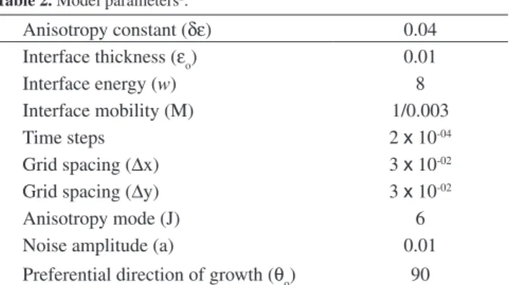
Table 2. Model parameters2.
Anisotropy constant (δε) 0.04
Interface thickness (εo) 0.01
Interface energy (w) 8
Interface mobility (M) 1/0.003
Time steps 2 x 10-04
Grid spacing (Dx) 3 x 10-02
Grid spacing (Dy) 3 x 10-02
Anisotropy mode (J) 6
Noise amplitude (a) 0.01
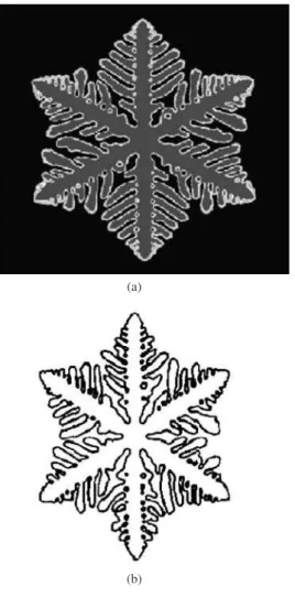
Figure 2a depicts the simulation of a nickel dendrite calculated here with a numerical grid of 1200 x 1200 points, while Figure 2b depicts the results obtained by Kim et al.6. A “seed” was set at the top left-hand corner, as done before by Kim et al.6. Both figures show: a) the secondary and tertiary arms; b) the secondary arm increases with the distance behind the primary dendrite tip; and c) the asym-metry in the side branch found in the secondary and tertiary arms. The initial and boundaries conditions we used in this simulation are identical to those adopted by Kim et al.6
4.2. Simulation of the solidification of a pure metal without
supercooling
Table 3 summarizes the values of the model’s parameters used here to simulate a nickel dendrite, while Table 4 lists the values of the material’s properties.
The initial temperature of liquid nickel was set to equal its melting temperature (Tm = 1728 K). The domain discretization was a mesh of 600 x 600 points. The four boundaries were cooled at identical rates. The temperature in the region neighboring the domain is 300 K. The cooling rate obeys the convection law for heat transfer. The regions closer to domain boundaries present lower temperatures, since the system is being cooled at the boundaries at a prescribed heat transfer coefficient of h = 45 Wm-1 K-1.
A thin layer of solid (φ = 1) was placed on the left, right and top borders of the domain, while a rectangular layer of solid was placed
Table 3. Parameters model (Ni)6.
Anisotropy constant (δε) 0.025
Thickness interface (εo) 2.01 x 10⁻⁴ (J/m)1/2 Free energy factor (w) 0.61 x 10⁸ J/m3
Mobility interface (M) 13.47 m3/sJ
Grid spacing (Dx) 2 x 10-08 m
Grid spacing (Dy) 2 x 10-08 m
Time steps (Dt) 1 x 10-12 (s)
Noise amplitude factor (a) 0.025
(b)
Figure 1. a) Present calculation and b) Kobayashi’s Dendrite calculation2, both with DH = 1.6.
(a)
(b)
Figure 2. Dendrite calculated with a 1200 x 1200 point grid, where the den-drite started to grow from a seed at the top left-hand corner toward the bottom right-hand corner of the box. Solidification time was 6.26 x 10⁻⁷ s.
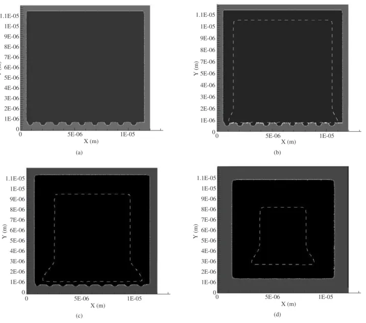
on the bottom border (Figure 3a). The objective of this simulation is to verify that, in a non-supercooled melt, the interface advances uniformly into the liquid region, with no branching. This type of plane interface is stable. These results are illustrated by the time evolution of the interface shown in Figures 3b to 3d.
The phase-field model is also able to reproduce solidification con-ditions in which the solid/liquid interface is stable and no dendrites are
(a)
Y (m)
2x 10⁻⁵
1.5x 10⁻⁵
1x 10⁻⁵
5x 10⁻⁶
0
0 1x 10⁻⁵ 2
x 10-5
Table 4. Properties material (Ni)6.
Interface energy (σ0) 0.37 J/m2
Coefficient kinetic interfacial 2 m/sK
Melting temperature (Tm) 1728 K
Latent heat (DH) 2.35 x 10⁹ J/m3
Thermal diffusivity (D) 1.55 x 10⁻⁵ m2/s
Specific heat (Cp) 5.42 x 10⁶ J/m3 K
Interface width (2λ0) 8 x 10-08 m
Figure 3. Development of the smooth interface from an initially disturbed region. Solidification time is a) t = 0; b) t = 6.9 x 10⁻⁹ s; c) t = 9.5
x 10-9 s; and d) t = 2.2 x 10⁻⁸ s, and the melting temperature isotherm (Tm = 1728 K) is also presented.
1.1E-05
1E-05
9E-06
8E-06
7E-06
6E-06
5E-06
4E-06
3E-06
2E-06
1E-06
0
Y (m)
0 5E-06 1E-05
X (m)
(a)
1.1E-05
1E-05
9E-06
8E-06
7E-06
5E-06
4E-06
3E-06
2E-06
1E-06
0
Y (m)
0 5E-06 1E-05
X (m)
(b)
1.1E-05
1E-05
9E-06
8E-06
7E-06
6E-06
5E-06
4E-06
3E-06
2E-06
1E-06
0
Y (m)
0 5E-06 1E-05
X (m)
(c)
1.1E-05
1E-05
9E-06
8E-06
7E-06
6E-06
5E-06
4E-06
3E-06
2E-06
1E-06
0
Y (m)
0 5E-06 1E-05
X (m)
(d)
formed. Such is the case of a pure metal that undergoes solidification due to heat extraction through the walls of a mould, with no supercool-ing of the bulk of the liquid. Under these circumstances, even large perturbations in the solid/liquid interface are damped and the solidifica-tion front becomes flat. Stabilizasolidifica-tion of a planar interface in a domain with no supercooling is also reported in Chalmers17 and is exemplified in Figure 3a-d, which shows the solid/liquid interface at four different moments during solidification. Figure 3a shows the initial condition,
where a pattern of rectangles was set as a seed for the solidification front. In Figure 3c-d, this pattern evolves to a planar front.
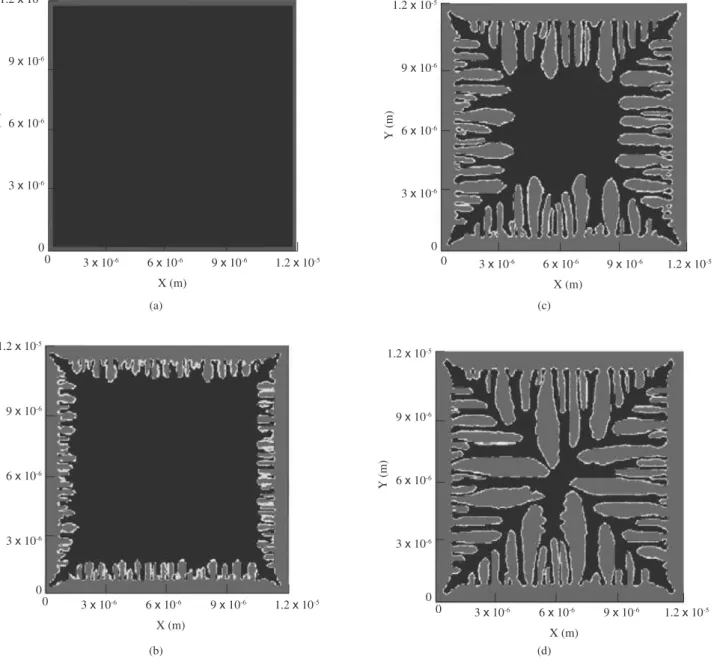
4.3. Solidification of a pure metal with supercooling effects
In this simulation, a fine solid layer was added to the domain boundaries and there is 260 K supercooling. The objective of this simulation is to demonstrate that the plane interface becomes unstable in a supercooled domain, with branching advancing into the liquid region. Figure 4a-d illustrates the advance of the interface. Note that regions close to domain corners solidify more slowly than other re-gions, which is due to the fact that there is a greater release of latent heat in the corners, causing the local temperature to increase and thus delaying solidification in this region. Figure 4d shows the primary arms; note that some of the arms located in the central region are well developed, including some secondary arms.
4.4. Solidification speed
of a linear dependence between the solidification speed and super-cooling17. A consequence of this assumption is the introduction of a constant linear kinetic coefficient, µk, in Equation 7. The coefficient µk
should be considered constant only for small ranges of supercooling. Disregarding this dependence could cause the linear behavior shown in Figure 5b. However, this assumption requires further investigation and will be the focus of the upcoming Ref. 18. However, the model predicted a velocity magnitude very close to that of the experimental results, especially at higher supercooling, where the experimental results scatter and do not rule out a linear behavior.
4.5. Development of the thermal field
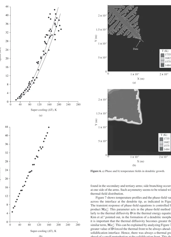
Figure 6a shows the solidification of initially supercooled (DT = 260 K) pure nickel with adiabatic boundary conditions and zero flux for φ, while Figure 6b shows the thermal field. In Figure 6a the dendrite started to grow from a solid nucleus at the top left-hand corner toward the bottom right-hand corner of the domain. One of the interesting phenomena is the asymmetry in the side branching
Figure 4. Evolution of an unstable interface into a supercooled melt. Solidification time is a) t = 0; b) 2.6 x 10⁻⁸ s; c) t = 7.5
x 10-8 s; and d) t = 4.6 x 10⁻⁷ s.
1.2x 10⁻⁵
9x 10⁻⁶
6x 10⁻⁶
3x 10⁻⁶
0
Y (m)
X (m)
0 3x 10⁻⁶ 6
x 10-6 9
x 10-6 1.2
x 10-5
(a)
1.2x 10⁻⁵
9x 10⁻⁶
6x 10⁻⁶
3x 10⁻⁶
Y (m)
X (m) 0
0
3x 10⁻⁶ 6
x 10-6 9
x 10-6 1.2
x 10-5
(c)
1.2x 10⁻⁵
9x 10⁻⁶
6x 10⁻⁶
3x 10⁻⁶
Y (m)
X (m) 0
0
3x 10⁻⁶ 6
x 10-6 9
x 10-6 1.2
x 10-5
(b)
1.2x 10⁻⁵
9x 10⁻⁶
6x 10⁻⁶
3x 10⁻⁶
Y (m)
X (m) 0
0
3x 10⁻⁶ 6
x 10-6 9
x 10-6 1.2
x 10-5
(d)
(a)
Data 2x 10⁻⁵
1.5x 10⁻⁵
1x 10⁻⁵
5x 10⁻⁶
0
Y (m)
0 1x 10⁻⁵ 2
x 10-5
X (m)
T (K) 1735 1682 1575 1484
(b)
T (K) 1735 1682 1575 1484 2x 10⁻⁵
1.5x 10⁻⁵
1x 10⁻⁵
5x 10⁻⁶
0
Y (m)
0 1x 10⁻⁵ 2
x 10-5
X (m)
44
40
36
32
28
24
20
16
12
8
4
0
0 40 80 120 160 200 240 280
Super-cooling ($T), K
Speed (m/s)
(a)
44
40
36
32
28
24
20
16
12
8
4
0
0 40 80 120 160 200 240 280
Super-cooling ($T), K
Speed (m/s)
(b)
Figure 5. Dendrite tip speed vs. thermal supercooling (DT), a) experimental17; and b) predicted in this work using the phase-field model.
Figure 6. a) Phase and b) temperature fields in dendritic growth.
found in the secondary and tertiary arms; side branching occurs only at one side of the arms. Such asymmetry seems to be related with the thermal-field distribution.
5. Conclusions
The phase-field model is a powerful tool for simulating details of solidification of crystalline materials. The model can be described as a transport-like equation for the solid phase formulated in terms of a phase-variable, φ, which determines whether the phase is solid or liquid. This transport equation was solved by a finite-volume scheme, explicit in time, together with a finite-volume scheme and an implicit-in-time scheme for the energy equation. The simulations of pure nickel dendrites carried out in this work were first compared with previous simulations reported in the literature to validate the present computational code. Calculations of the solidification of pure nickel were then used to investigate the model’s ability to reproduce both stable and unstable solid/liquid interfaces. Predictions of the phase-field method for the solidification velocities at dendrite tips were compared with data from the literature17. Our model was able to reproduce the general behavior and the predicted velocities were of the same order of magnitude found in experimental data. The phase-field model, however, could not reproduce the nonlinear dependence between solidification velocities and supercooling levels. The likely reason for this discrepancy was “built into” the phase-field model due to the use of a constant interface mobility, M, through a kinetic coefficient µk, originally postulated as a constant.
1
0.9
0.8
0.7
0.6
0.5
0.4
0.3
0.2
0.1
0
- 0.1
T
emperature (K)
1700
1650
1600
1550
1500
1.175E-05 1.2E-05 1.225E-05 1.225E-05
X (m)
V
ariable phase f
ield (
F
)
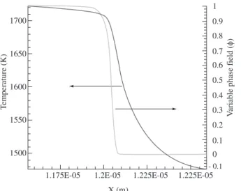
Figure 7. Temperature and phase-field variable profiles across the solid/liquid interface.
References
1. Caginalp G, Fife P. Phase-Field methods for interface boundaries. Physical Review B. 1986; 33:7792-7794.
2. Kobayashi R. Modeling and numerical simulations of dendritic crystal
growth. Physical D. 1993; 63:410-423.
3. Andersson C. Phase-Field simulation of dendritic solidification. [Unpub-lished PhD Thesis]. Stockholm: Royal Institute of Technology; 2002.
4. McFadden GB, Wheeler AA, Braun RJ, Coeriell SR. Phase-Field model for anisotropic interfaces. Physical Review E. 1993; 48:2016-2024.
5. Wheeler AA, Murray BT, Schaefer RJ. Computation of dendrites using
a phase-field model. Physical D. 1993; 66:243-262.
6. Kim SG, Kim WT, Lee JS, Ode M, Suzuki T. Large scale simulation of dendritic growth in pure undercooled melt by phase-field model. ISIJ International. 1999; 39(4):335-340.
7. Boettinger WJ, Warren JA, Beckermann C, Karma A. Phase-field simulation of solidification. Annual Review of Materials Research. 2002; 32:163-194.
8. Warren JA, Boettinger WJ. Prediction of dendritic growth and micro-segregation patterns in a binary alloy using the phase-field method. Acta Metallurgical Materials. 1995; 43(2):689-703.
9. Lee JS, Suzuki T. Numerical simulation of isothermal dendritic growth by phase-field model. ISIJ International. 1999; 39(3):246-252.
10. Ode M, Suzuki T. Numerical simulation of initial microstructure evolu-tion Fe-C alloys using a phase-field model. ISIJ International. 2002; 42(4):368-374.
11. Ode M, Lee JS, Kim SG, Kim WT, Suzuki T. Phase-field model for so-lidification of ternary alloys. ISIJ International. 2000; 40(9):870-876.
12. Ode M, Kim SG, Kim WT. Suzuki T. Numerical prediction of the second-ary dendrite arm spacing using a phase-field model. ISIJ International. 2001; 42(4):345-349.
13. Ode M, Suzuki T, Kim SG, Kim WT. Phase-field model for solidification
of Fe-C alloys. Science and Technology of Advanced Materials. 2000;
1:43-49.
14. Kim SG, Kim WT, Suzuki T. Phase-field model for binary alloys. Physical Review E. 1999; 60(6):7186-7197.
15. Kim SG, Kim WT, Suzuki T. Interfacial compositions of solid and liquid in a phase-field model with finite interface thickness for isothermal solidi-fication in binary alloys. Physical Review E. 1998; 58(3):3316-3323.
16. Patankar SV. Numerical Heat Transfer and Fluid Flow.
McGraw-Hill-Hemisphere Publication, Minnesota, USA, 1979.
17. Chalmers B. Principles of Solidification, USA: John Wiley & Sons; 1964.
Appendix
From the hypothesis of equilibrium, a solution exists when T=Tm for a one-dimensional transition zone between liquid (φ=0) and solid (φ=0), where φ varies in the x direction normal to the interface. In this case, Equation 1 becomes:
dx d
w d dg
2 2 2 f z
z z
= _ i (10)
g(φ) is here represented as follows:
g(φ) = φ2 (1 – φ)2 (11)
and
d dg
2 1 1 2
z z
z z z
= -
-_ i _ i_ i (12)
Inserting Equation 12 into 10, one has:
dx
d 2w
1 1 2
2 2
2 z
f z
z z
= _ - i_ - i (13)
The solution is:
tgh w x
2 1
1
2
o
z
f
= > - e oH (14)
The goal here is to show that Equation 14 is a solution of Equa-tion 13 and that it satisfies the boundary condiEqua-tions, where φ = 1 (solid) when x → - ∞ and φ = 0 (liquid) when x → + ∞. Rearranging Equation 14,
tgh w x
2f = 1-2zo
e o (15)
The relation between the hyperbolic functions is:
sech w x tgh w x
2 1 2
2 2
f = - f
e o e o (16)
Taking Equation 15 into Equation 16,
sech w x
2 1 1 2 o
2 2
f = - - z
e o _ i (17)
Differentiating Equation 14 twice:
sec tanh
dx
d w w
x w x
2 h 2 2
2 2
2 2
2 $ z
f f f
= f p e o (18)
Using Equations 15 and 16 in 17 and rearranging the terms, one has:
dx
d 2w
1 1 2
2 2
2 z
f z
z z
= _ - i_ - i (19)