Automated Detection of Bone structure keypoints on Magnetic Resonance imaging - Sternum and Clavicles

(1)

FACULDADE DE

ENGENHARIA DA

UNIVERSIDADE DO

PORTO

Automated Detection of Bone structure

Keypoints on Magnetic Resonance

Imaging - Sternum and Clavicles

Beatriz Gonçalves Rocha

MESTRADO INTEGRADO EM BIOENGENHARIA- ENGENHARIA BIOMÉDICA Supervisor: Hélder Filipe Pinto de Oliveira

Co-Supervisor: João Pedro Fonseca Teixeira

(2)

c

(3)

Abstract

Breast cancer is one of the most prevalent types of carcinogenic diseases worldwide, meaning that is a pathology very appealing to be explored in terms of cure and methods to help the diagnose and treatment processes.

With the evolution of technology applied to science, much work has been developed in order to find solutions to improve the treatments of pathologies like breast cancer. One of those, relates to this dissertation work, where a strategy for personalized surgical treatment is being explored in order to increase the quality of life for the patients who have to be submitted to oncoplastic surgical procedures.

This dissertation work, focuses on the automatic segmentation of the Sternum and the Clav-icles in Magnetic Resonance Imaging (MRI). The identification of these specific bones will be used as reference to help a three dimensional reconstruction of patient digital model through their individual MRI acquisition. To achieve this, is important to have body structures identified in the acquisitions such as bones to serve as reference to create the individual radiological atlas and multi-modal fusion.

The segmentation of this structures proposed is achieved using the gradient of the images elliptically transformed, where the boundaries are emphasized. The minimum cost pixel path, after an intensity modification, is estimated and corresponds to the object contours. Classification approaches using Support Vector Machine and Random Forest models were also tested, using different sets of features extracted.

The dataset used in this work had 14 MRI T1-weighted breast cancer patient acquisitions, from their thoracic area. The classification methods for the sternum the clavicles achieved Dice Similarity Coefficient (DSC) of 0.087 and 0.25. In the gradient based segmentation the DSC was 0.58 for the sternum and 0.36 for clavicles.

The developed method, based on image gradient to detect the objects after being transformed, revealed to be a great disclosure to achieve the sternum and clavicles automated detection in MRI. It is a promising starting point to develop a robust segmentation method for these bones.

(4)

(5)

Acknowledgements

This dissertation represents the culmination of long five years.

They were certainly the most intense years of my life, so far, and I am grateful that I embrace this opportunity.

Firstly, I would like to thank my supervisors, João Pedro Teixeira and Hélder Oliveira, for playing a crucial role during the development of this work, guiding and encouraging me. This work was funded by the ERDF - European Regional Development Fund through the Norte Por-tugal Regional Operational Programme (NORTE 2020), under the PORTUGAL 2020 Partnership Agreement and through the Portuguese National Innovation Agency (ANI) as a part of project BCCT.Plan–NORTE-01-0247-FEDER-01768.

I would like to thank all my Professors. Beginning in my Pre and Elementary school teachers, Leninha and Susana, to every High School and University Professors. All of you, somehow, taught me something that I will carry for my life.

I would also like to thank all my friends, especially the ones that had to deal with me and my moods during this process. Thank you for cheering me up, even in my darkest days. I know it was not easy, but I at least hope it was funny.

I would also like to give a special thanks to my friends who welcome me in my first days in university. Those were not easy days, with many doubts and insecurities about my choices, but with your help I managed to finish my degree in five years!

At last, but definitely not least important, I would like to give the biggest thanks my family. Without them I would never have the possibility to even dream to achieve this. My real, Marcos and Mizé, and fake uncles, Amélia e João for always be there for me, when I needed the most. My cousin, Mariana, for being my partner in everything during this past year. Also, my grandparents, Alice and Rodolfo who accommodate me and my bad moods and always missed me when I was not home, and my grandfather Henrique for always support me during weekend quick visits and lunches. My stepmother, Zélia for the understanding about dealing with engineering courses. My brother, Francisco, who grow up watching me studying to achieve this. Thank you for all the times you distract me and made me realize that there are things much more important and unique than work. I hope I will help you in your journey even more than you helped me. My mother and father! Without whom I could not even image to pass the elementary school. I want to give you the biggest thank you, from the bottom of my heart, for all the support. Despite every distance, you were always there for me. Thank for not giving up on me and on my insecurities, tears, mournings and fears. I hope I made and will always make you proud!

All of you shaped the person I become today. I don’t know what is coming next, but I hope I will count on you for many years more and you will help me reaching other things that seem impossible for me now to accomplish.

Beatriz Gonçalves Rocha.

(6)

(7)

“Science works on the frontier between knowledge and ignorance. We’re not afraid to admit what we don’t know. There’s no shame in that. The only shame is to pretend that we have all the answers.”

Neil deGrasse Tyson, Cosmos: A Spacetime Odyssey.

(8)

(9)

List of Figures

1.1 Global distribution estimated age-standardized of female breast cancer (a) and its

incidence worldwide (b)Imaging[2018]. . . 1

2.1 Ken Saladin[2003] representation of Sternum . . . 6

2.2 Ken Saladin[2003] representation of Clavicles . . . 7

2.3 Ken Saladin[2003] representation of the Thoracic Cage and Pectoral Girdle . . . 8

2.4 MRI acquisition representation [Reeve,2018]. . . 9

2.5 MR image example from an axial cut. . . 10

2.6 Dam et al.[2015] algorithm scheme . . . 15

2.7 Balsiger et al.[2015] algorithm scheme . . . 17

2.8 Bourgeat et al.[2006] representation of the Gabor bank filter. . . 20

2.9 Lu et al.[2006] algorithm iteration demonstration from a) to e) . . . 21

2.10 Oliveira et al.[2012] algorithm demonstration comparing the ground truth (solid red line) and the detected contour (dashed white line), zoomed on the right. . . . 22

3.1 General Feature extraction and Classification methods pipeline. . . 26

3.2 Magnitude (a) and phase (b) representations of chest MRI in axial cut. . . 27

3.3 Balsiger et al.[2015] preprocessing on MRI chest acquisitions. . . 28

3.4 Gradient based segmentation method pipeline. . . 30

3.5 Sternum segmentation detailed pipeline. . . 31

3.6 Clavicles detection detailed pipeline. . . 32

3.7 MR slice in the axial cut. . . 32

3.8 Otsu threshold with sternum roughly defined limits in the center axial view. . . . 33

3.9 Sagittal view of the sternum (a) and its correspondent gradient image (b). . . 34

3.10 Initial point definition based on central profiles representation. . . 34

3.11 ROI limits representation. . . 35

3.12 ROI example. . . 35

3.13 MR image containing clavicles. . . 36

3.14 ROI clavicles examples from left (a) and (b) right side. . . 36

3.15 Sternum shapes detected after object selection (a) and the correspondent content (b). 37 3.16 ROI clavicle representation (a) and the correspondent Canny filter application (b). 38 3.17 Detected objects after Canny edges filling (a) and correspondent clavicle selection (b). . . 38

3.18 Ellipse representation [Therézio et al.,2017]. . . 39

3.19 Two different sternum ROI examples. . . 41

3.20 Correspondent two elliptical transformation examples. . . 41

3.21 Minimum paths pipeline. . . 42

3.22 Sternum compressed coronal view. . . 42

(12)

x LIST OF FIGURES

3.23 RG coronal mask to identify the sternum content slices. . . 43

4.1 Minimum path result for sternum contour fisrt example. . . 49

4.2 Minimum path result for sternum contour second example. . . 49

4.3 Minimum path result for sternum contour third example. . . 50

4.4 Minimum path result for clavicle contour first example. . . 50

4.5 Minimum path result for clavicle contour second example. . . 51

4.6 Minimum path result for clavicle contour thrid example. . . 51

4.7 SVM and RF classification methods in Bourgeat et al.[2007] andBalsiger et al. [2015] features results in sternum compared to the ground truth. . . 52

4.8 SVM and RF classification methods in Bourgeat et al.[2007] andBalsiger et al. [2015] features results in clavicles compared to the ground truth. . . 53

4.9 Minimum paths missing sternum contours. . . 54

(13)

List of Tables

2.1 Review on Segmentation techniques for MRI leg images [Gandhamal et al.,2017]. 13

4.1 Bourgeat et al.[2007] methodology implementation results for sternum identifica-tion. . . 47

4.2 Balsiger et al.[2015] methodology implementation results for sternum segmentation. 47

4.3 Bourgeat et al.[2007] methodology implementation results for clavicle identifica-tion. . . 48

4.4 Balsiger et al.[2015] methodology implementation results for Clavicles identifi-cation. . . 48

4.5 Gradient based sternum segmentation results. . . 50

4.6 Minimum path result for clavicle contour example. . . 51

(14)

(15)

Abbreviations and Symbols

2D Two Dimensional 3D Three Dimensional AAM Active Appearance Model ASM Active Shape Model AvgD Average Distance

BCCT Breast Cancer Conserving Therapy CT Computed Tomography

DRLSE Distance Regularized Level Set Evolution DSC Dice Similarity Coefficient

FN False Negative FP False Positive

GAC Geodesic Active Contours GC Graph minimum-Cut

GLCM Grey-Level Co-occurrence Matrix k-NN k Nearest Neighbors

LDA Linear Discriminant Analysis LWV Locally Weighted Vote MR Magnetic Resonance

MRI Magnetic Resonance Imaging MSE Mean Square Error

PDM Point Distribution Model RF Random Forest

RG Region Growing

RMSD Root Mean Square Distance ROI Region of Interest

Sens Sensitivity

SNR Signal to Noise Ratio Spec Specificity

SSM Statistic Shape Model SVM Support Vector Machine TN True Negative

TP True Positive

(16)

(17)

Chapter 1

Introduction

1.1 Context

Breast cancer is one of the most common types of cancer worldwide. Among female population, is the most prevalent cause of death as a non-skin type of cancer. The statistics from 2012 indicated that there were about 1.60 million new diagnoses and 0.52 million deaths caused by this type of cancer. Demographic changes related to the population growth and regional risks are indicated as the main factors to the increasing of the disease burden (Figure1.1) .

Figure 1.1: Global distribution estimated age-standardized of female breast cancer (a) and its incidence worldwide (b)Imaging[2018].

Being the incidence higher in Western countries, the burden of the disease is major located in East and Central Asia, with 41.5% of deaths and 36.3% of the cases. In Europe, the statistics for diagnosis and deaths is about 25%. In general, though the years between 1994 and 2012 the incidence of the cancer has been increasing 0.6% per year between women at ages of 20 to 39. The mortality rate has been declining due to the combination of treatment improvements and the early detection but still high: 21.52%. The risks of developing this cancer relies mainly on the genetic predisposition and some habits like the alcohol consumption and unhealthy weight [Imaging,2018].

(18)

2 Introduction

Cancer is characterized as being the presence of a malignant tumor, which is an abnormal development of cells that creates a mass of tissue. There are a few treatments available nowadays to try to eliminate that, being its early detection and treatment options largely studied. Many of the treatments rely on chemical attack to the tumor, however some patients still need to fight it physically, removing the tumor itself. In the case of breast surgery, it is removed part or the entire breast where the tumor relies, in order to help to overcome the pathology.

The decisions to be made concerning the treatment are numerous, complex and differ from patient to patient. They still rely almost exclusively on the perspective of the surgeon, concerning the post-surgical aesthetic result.

1.2 Motivation

The fact that the breast cancer mortality rates have been decreasing, makes that many survivors still have to deal with the consequences of the disease treatment for a considerable amount of their lives. In particular, the breast surgery consequences usually are related with the psychological recovery which can be compromised if the patient rejects or stays unsatisfied with the aesthetic result.

Breast cancer conservative treatment (BCCT) came as an alternative to the traditional mastec-tomy, having the main objective of locally control the tumor, having the same positive results of the traditional surgery but taking in consideration a satisfactory aesthetic result.

Some decisions concerning the surgery remain on the physician’s perspective, leading some-times to unsatisfactory outcomes due to the fact of being a quite subjective analysis due to the lack of concrete visualization of the anatomical condition of the patient and the lack of methods to keep the patient involved in the process.

An objective evaluation of the process and its results would improve these techniques, increas-ing the objectivity, reproducibility and the communication between the physician and the patient.

Developing a three dimensional (3D) individual model of the breast area enables the achieve-ment of a better perspective on the surgical options and their consequences, being an evident alternative to the current methodology. It would allow a better surgery planning, giving the dig-ital model of the body structures through a large number of angles. I would also provide a vol-ume/volume deficit estimation and it would allow the patients to get more involved and understand better the procedures and the possible results [Oliveira et al.,2014].

The conceptualization of this 3D model relies on the digital reconstitution of the patient body structures based on their Magnetic Resonance (MR) images. Together with an external reconstitu-tion, the inner parts of the body have to be connected with the external ones. To achieve that, it is necessary an automatic identification of some keypoints in the MRI acquisitions to connect these two reconstituted parts of the patient. With this kind of personalized model, it would provide tools to perform the digital examination and surgery planning in a more objective and realist way.

(19)

1.3 Objectives 3

1.3 Objectives

This dissertation work was developed in line with the goals of the Portugal2020 BCCT.Plan Project, where tools for clinical teams are being built and different strategies for personalized surgical treatment for patients are being explored. This will allow to adjust and plan each surgery. This project is inserted in a three years partnership between INESC TEC, the Champalimaud Foundation and NEADVANCE.

It will take in consideration the MR images from each oncologic breast patients that were subjected to an oncoplastic surgery. From this scan, there are many structures that can be detected in those images. Some can be considered as references for the 3D reconstruction, working as key points to guide the digital model creation.

In this dissertation, the human skeleton is the main part considered. In particular, the Clavicles and the Sternum automatic detection is the main objective of this work. The detection of these bones will help in the reconstitution of each 3D model, giving reference keypoints to provide the precision of multi-modal registration tasks. As they are the most superficial bones, in this area, they will support the connection of the most external reconstituted body parts with the internal content.

1.4 Contributions

With this dissertation work, it is expected to develop a technique to automatically identify the sternum and the clavicles in T1-weighted MR volumes which will constitute a new tool to help achieve the main research line objectives of the project where this dissertation is inserted. The automatic detection of this structures will provide the model in development key points to serve as reference in the process of transformation the MRI acquisitions into a digital 3D model.

A scientific paper was also written, focusing on the sternum segmentation. This achievement also has the potential to be a new approach in the biomedical imaging science field, since the most common techniques for bone chest detection use X-Ray images. This method can become useful for other applications where the detection of this bones in MRI is necessary or even to serve as inspiration for other object detection in similar conditions.

1.5 Structure

The present document is a dissertation work. It is divided in the following chapters and topics: The Chapter2, has two main sections. The Background is where the main concepts that sup-port the whole work are explained and described. In the section of the Segmentation Techniques the algorithms already described in the literature, that are somehow related to this work, are pre-sented and the ones that can be more relevant for the desired implementation are explained. At the end of this chapter, a brief summary is made.

(20)

4 Introduction

In Chapter3it is made a short introduction to contextualize the implementation process. Clas-sification methods applied during the dissertation work are exposed. The last section is the de-scription of the gradient based method, which explains an algorithm developed to segment each structure (sternum and clavicles) to achieve the intended objective.

In Chapter4an initial characterization of the dataset that was used to test the algorithms is made. Then, the results are exposed through tables with statistical measures used to evaluate the performance of the methods and some visual examples are also exposed. After that, the results are explained and justified during the Discussion section.

In the final Chapter,5, the conclusions of the work developed are made and the possible future approaches and improvements are referred.

(21)

Chapter 2

Literature Review

2.1 Medical and Anatomical Background

It is important to understand the theoretical components of the topics that are going to be addressed during this dissertation work to understand better its characteristics, the way the structures appear in the images, their shape and constitution and the technique involved in their acquisition.

2.1.1 Bone Structure

Bone is a hard connective tissue with matrix (mineralized) and cells (living part). Its matrix con-sists of collagen fibers, the organic portion, and hydroxyapatite, the inorganic portion containing calcium and phosphate.

There are two types of bone structure: the compact and the cancellous one. The compact bone is composed by osteons, it is hard and dense, making the outside surface and the shaft of long bones. The spongy one has a thin and irregular shaped plate called trabeculae, arranged in a lattice work, being less dense.

Bones have rich blood supply which provides them the capacity to repair themselves quicker than other parts like cartilage [Rod Seeley and Philip Tate,2003].

2.1.2 Skeletal System

The skeletal system is constituted by all of the bones and joints present in the whole body, being the solid framework that supports, protects and anchors the rest of the body parts. It has two distinctive portions: the axial and the appendicular skeleton, being the axial constituted by a total of eighty bones. It includes the vertebral column, the rib cage and the skull. The appendicular has a total of one hundred and twenty-six bones composed by the remaining ones.

The skeleton acts as a scaffold to provide support, it protects organs and the soft tissues that surrounds, it is an attachment points provider for muscles allowing movement at the joints and it also owns nerves and the production of new cells that occurs in the red marrow. It is located inside of bones in their medulla cavities, transforming in yellow bone marrow through adulthood

(22)

6 Literature Review

and storing energy in lipidic forms. It also stores different type of essential elements like calcium, iron and and hormones to help the growth and body repair.

The skeleton expands throughout childhood being the foundation for the other body parts to grow along with. It begins to form in fetal development as a hyaline cartilage and dense irregular connective tissue which makes the structure flexible being a soft framework and a placeholder for the future replacement osseous tissue (calcification)[Rod Seeley and Philip Tate, 2003,Ken Saladin,2003].

2.1.3 Sternum

The sternum is a component of the thoracic cage region of the skeleton, as represented in the Figure2.3, articulating with the right and left clavicle and some ribs. It is a long, narrow flat bone located at the anterior aspect of the thorax and the heart, lies in the mid-line of the chest and has a shape roughly similar to a “T”. It is composed by three pieces: the manubrium, the body and the xiphoid process (Figure2.2).

In average, a sternum has about 15 to 20 centimeters length, and 2.5 centimeters wide and thick, and it is a bone mainly spongious and highly vascularized due to the presence of red marrow in its interior. The sternum is commonly known as the breastbone, since it serves as keystone for the rib cage, connecting with it, and stabilizes the thoracic skeleton. It also gives protection for several vital components located in the chest such as the heart, lungs, thymus gland, aorta and vena cava. There are many muscles that allow movements of the arms, neck and head that derive from the sternum.

(23)

2.1 Medical and Anatomical Background 7

The manubrium part has a superior concave shape, with a depression denominated as jugular notch which articulates with the medial ends of the clavicles to form the sternoclavicular joints. On the lateral edges of the manubrium, there is a facet that articulates with the costal cartilage of the first rib and a demifacet to articulate with part of the costal cartilage of the second rib. In the lowest part it forms the sternal angle to articulate with the body part of sternum.

The body is the longest part of the sternum and has an irregular rectangular shape. Some costal cartilages of ribs, starting from the second one, connect there forming the bulk of the rib cage. Also, in this part are slight indentations, the articular facets, to provide the attachment points for the costal cartilages, preventing rib separation.

The xiphoid process is the smallest and the most inferior region of the sternum and it has a variable shape and size. It is not always an ossified part of the body: in the early life stays as a flexible hyaline cartilage region and ossifies throughout childhood and adulthood until around the age of 40 when all its cartilage is replaced by bone. Regardless of its degree of ossification, serves as an important point for attachment diaphragm tendons and of abdominal muscles such as rectus abdominis, and transversus abdominis [Rod Seeley and Philip Tate,2003,Ken Saladin,2003].

2.1.4 Clavicle

The clavicle is a slender bone, as represented in the Figure2.3, classified as a long bone having a slightly “S” shape. It has three main functions: attachment, protection and force transmission. Being convex in the medial aspect from the front view and concave from the lateral, it is crucial to sustain the forces applied from the pectoralis muscles and can be divided in two ends (the sternal and the acromial) and a shaft.

Figure 2.2:Ken Saladin[2003] representation of Clavicles

The sternal end contains a facet to articulate with the manubrium of the sternum in the ster-noclavicular joint. It has a rough oval depression in the inferior surface for the costoclavicular ligament. The acromial end has a small facet to articulate with acromion of the scapula and serves as attachment for two ligaments: the conoid tubercle and the trapezoid line.

It is doubly present in a normal human body, being each clavicle (right and left) connected to the sternum by their sternal ends [Ken Saladin,2003,Rod Seeley and Philip Tate,2003].

(24)

8 Literature Review

Figure 2.3:Ken Saladin[2003] representation of the Thoracic Cage and Pectoral Girdle

2.1.5 Magnetic Resonance Imaging

Magnetic Resonance (MR) was firstly developed as a superior computed tomography (CT) scan-ning technique, in 1970s, to visualize soft tissues.

By definition, magnetic resonance is a property of the elements that when submitted to a magnetic strong field and excited by radio waves in a specific frequency (Lamor frequency), they emit radio signal that can be captured by aerials or transformed into images.

Protons and neutrons have a property called spin or angular momentum which is a rotation around their own axis, having the protons also a magnetic moment which allows them to behave like a magnet. A magnetic moment, present in every proton, not only produces a magnetic field but also reacts to any other exterior magnetic field, so protons can be excited by powerful magnets producing a strong magnetic field changing the direction of the rotational axis.

Magnetic resonance imaging (MRI) uses a powerful magnetic field, radio frequency pulses and a computer to produce three dimensional detailed anatomical images being used to help the detection, diagnosis and monitoring of many conditions located in the chest, abdomen and pelvis. It is a non-invasive exam, without any ionizing radiation being an advantage comparing to other tools, and it can produce detailed images of every kind of body structures: organs, soft tissues and bones.

To acquire this kind of exam, the patient lies inside a large cyllindrical magnet chamber and has to remain still to avoid blurring the images (Figure 2.4). The environment creates a strong magnet field (3000 to 6000 stronger than the field of the Earth). Often, an intravenous contrast agent is given to the patient to increase the brightness in the resulting images.

When the radio waves reach the patient, the protons of hydrogen present in the body are stimulated and spin out of their equilibrium, aligning with the magnetic field. Then, when the

(25)

2.1 Medical and Anatomical Background 9

Figure 2.4: MRI acquisition representation [Reeve,2018].

radio frequency is turned off, the sensors capture the energy released while the protons abruptly realign. The time taken to align with the magnetic field, the amount of energy released, and time spent to realign, called the relaxation time, depend on the environment and on chemical nature of the molecules, allowing to differentiate tissues by their magnetic properties.

Since the hydrogen has only a single proton it has the ability to produce the largest radio signal. It is an element very abundant in the human body, integrating the water molecule structure, it is the most suitable for the magnetic resonance image capture where the signal is produced by its magnetic moment after the realignment.

Tissues have different relaxation times, and the kind of acquisition is determined by the type of relaxation that is captured: T1 is the longitudinal one and T2 the transverse. This is what creates the images, being the relaxation times chosen the predominant source of contrast. T1-weighted images are the ones created by the longitudinal relaxation time acquisitions. They were chosen to be explored in this work since they are the most common technique used to chest MRI, providing better anatomic detail. They are characterized by the high magnetization from the tissues that have a lower relaxation time, being the brightest parts in the images. In this kind of acquisition, bones appear as dark parts, muscles with gray tones, bone marrow equal or brighter than muscles, fat with the brighter appearance and air is dark [Ken Saladin,2003,Paul B, Adam M,2007,Hage and Iwasaki,2009].

(26)

10 Literature Review

as bones, showing complex structures which can lead to the presence of inadequate brightness and poor contrast in boundaries between hard and soft types of tissues [Gandhamal et al.,2017].

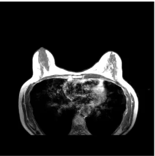
In long bones, like clavicle, the cortical bone thins out closer to the joints depending on the imaging process parameters, such as noise, bias fields and the partial volume effect. This makes the boundaries with other kind of bone and tissues more prone to be blurred, leading to segmentation issues and errors since none of the MR contrasts mode provide clear delineation (Figure2.5) [Dam et al.,2015].

Figure 2.5: MR image example from an axial cut.

2.2 Segmentation Techniques

Today, there are many techniques already developed to segment bone parts in MRI but to the best of our knowledge, there are not techniques specifically to the bones of interest in this work: the sternum and the clavicles and for this particular acquisition setup.

Despite that, it is important to acknowledge the work already done and published in this field in order to understand which are the best candidate approaches to the achieve the aim of this work. For that, it will be taken in consideration the techniques that have already shown to produce relevant results.

2.2.1 MRI Bone Segmentation

There are some interesting approaches to general MRI bone segmentation, although not directly applicable, they allow extracting concrete information or segmenting a specific bone or body struc-ture.

(27)

2.2 Segmentation Techniques 11

Hofmann et al. [2011] proposes a segmentation algorithm that combines image thresholds, Dixon fat–water segmentation, and component analysis to detect the lungs, in MRI from the whole body, acquired with patients with their arms up. The data preparation involves a low pass filter using a Gaussian kernel and morphological operations to eliminate information from the regions outside of the body of the patients. The segmentation itself includes a 5-class approach: air, lungs, fat tissue, fat and non-fat mixture and water where is applied a intensity based thresholding. Air and non-fat tissue were separated by thresholding the intensity-normalized in-phase images. Low intensity voxels were set as air with the help of a close operation to avoid misclassification. Fat and water voxels were separated based on Dixon images, being the fat characterized by having more than the double of the intensity value comparing to the water ones. The lungs were detectable as the largest connected group of low intensity voxels.

To segment bone parts present in MRI, Schmid et al.[2011], presented his approach which involves the use of statistical shape models (SSM). The process involves the creation of the SSM with a training set of shapes that resulted from images that were progressively segmented by a deforming template mesh guided by a radiologist. The statistics were inferred by this process. The initialization process attempts to find the best pair of rigid transform and shape parameters that minimize a cost function and its evolution is based on forces that are applied to these particles. The resulting discrete differential equations are solved by a stable Euler implicit numerical scheme. The external image forces appeal to go towards the desired boundaries by using image features, in order to isolate the desired objects.

To a semi-automatic approach,Ozdemir et al.[2017] described the use of the random forests classifier to train the model and a random walker algorithm to segment bone regions. It extracts statistical features from different orders using cubic patches of edge length centered at each voxel: the mean, the variance, the skewness and the kurtosis making a total of 12 features dimension. Also, the texture and curvature maps are extracted with the Gabor filters and anisotropic features to pronounce different orientation structures, especially in cancellous and cortical bone and their surrounding muscles. It is also referred the relevance of extracting context-integrating and lo-cation features in the proximity of the humerus since the shoulder has a dense constitution of muscles, tendons and fat. It incorporates contextual information of the spatial neighborhood and spatial shifts at multiple scales of different image maps. They were previously smoothed with a cubic kernel, to have relative orientation and distance-dependent information for each voxel that will help to characterize this kind of areas. For the segmentation, the random walker algorithm was chosen, being necessary to select the seed points and pairwise edge weights to perform the labelling to each voxel.

2.2.2 MRI Leg Bones segmentation

The majority work developed in the MRI bone segmentation field targets leg bones, such as the femur, the tibia and the patella.

(28)

Given the diversity of approaches already developed and reported, it is interesting to explore if any of those works use techniques that could be applied in the present work, or even if several techniques may be combined to produce better results.

In a paper byGandhamal et al.[2017], beyond presenting their own approach for knee bone segmentation, a review on the existing techniques is made. This is shown in Table2.1.

The main technique categories presented in the table are going to be explained and the ones with the most interesting contents are going to be described.

2.2.2.1 Semi-Automatic Techniques

Although semi-automatic algorithms may not be directly the intended approach for this work, they can contain some techniques that could be useful to understand the segmentation approaches already done.

A semi-automatic method is intended as a method in which in some phase of the process they require the use intervention. Usually, in this kind of approaches, the interaction occurs on the initial segmentation stage, to be chosen the starting points (seeds) on the regions of interest to give a reference for the segmentation initialization. This restriction leads to reliability issues, being a limitation of the performance of the algorithms, making them unsuitable for many purposes [Gandhamal et al.,2017].

Distribution and Texture-based active contours

From both methods presented in the compilation table the one proposed inGuo et al.[2011] has reported the best performance, evaluated using Dice Similarity Coefficient (DSC).

They present a hybrid active contour model in order to compensate the individual limitations of both methods that were fused: Geodesic active contours (GAC) model and histogram based Bhattacharyya gradient flow. The GAC model is an energy active contours model based on the classical snakes and uses the statistical overlap constrain to prevent method to the boundary’s leak-age, improving the image segmentation performance. The use of Bhattacharyya distance relates to the search for mismatched zones. It corresponds to boundaries between objects and background, such that were the distance value is bigger the greater is the probability that functions are different and correspond to a boundary.

Multiphase Chan-Vese model

InJiang et al.[2008], an approach using the Chan-Vese model was proposed. It is a region-based deformable method for active contours region-based on energy minimization. It can detect objects whose boundaries are not necessarily well defined by the gradient but has the problem that can only isolate two scales of intensity of the image. To fight that, the Chan-Vese is used as the basal algorithm and then two improvements are performed. The multiphase Chan-Vese model is first applied and divides the images into two intensity regions, then, based on the type of intensity variance in the region, an area term is added to set the initial curves and regulate them. Finally,

(29)

2.2 Se gmentation T echniques 13

Table 2.1: Review on Segmentation techniques for MRI leg images [Gandhamal et al.,2017].

Type Key Segmentation Algorithms Author, Year Performance Metrics Dependability

Semi-automatic

Distribution and Texture-based active contours [Guo et al.,2011] DSC- 0.94

Depends on users for seed or contour initialization

Lorigo et al., 1998 DSC- 0.89

Multi-phase Chan-Vese Model [Jiang et al.,2008] not specified

Thresholding and Adaptative Region Growing, Bayesian Classification

[Dalvi et al.,2007] (Femur) Sens.- 97.05, Spec.- 98.75 (Tibia) Sens.- 96.95, Spec.- 98.33

Lee et al., 2005 Not specified

Kapur et al., 1998 Not specified

Fully-automatic

Multi-atlas registration and voxel classification

Tamez-Pena et al., 2016 (Femur) DSC – 0.95

(Tibia) DSC – 0.95

Most algorithms depend on models, atlas designs and training dataset set for classification [Dam et al.,2015] DSC – 0.97

[Lee et al.,2014] (Femur) AvgD–0.63 mm, RMSD–1.05 mm (Tibia) AvgD–0.53 mm, RMSD– 0.90 mm

Shan et al., 2014 (Femur)DSC – 0.96

(Tibia) DSC – 0.96

Graph Cut Algorithm [Ababneh et al.,2011] DSC – 0.95

Ray Casting technique Dodin et al., 2011 (Femur) DSC – 0.94

(Tibia) DSC – 0.92 Random and Semantic Context Forests Learning [Balsiger et al.,2015] DSC– 0.92

Wang et al., 2013

(Femur) DSC – 0.94 (Tibia) DSC – 0.95 (Patella) DSC – 0.94

Active and Statistical Shape Models, Appearance Models

[Neogi et al.,2013] Not specified

Bindernagel et al., 2011 (Femur) DSC – 0.94

(Tibia) DSC – 0.89 Seim et al., 2010 (Femur) AvgD – 1.02 mm, RMSD– 1.54mm (Tibia) AvgD – 0.84 mm, RMSD – 1.24 mm Williams et al., 2010 (Surface)Seg. Err. – 0.648

(Volume)Seg. Err. – 0.431 [Fripp et al.,2007] (Femur) DSC – 0.96

(Tibia) DSC – 0.96 Phase information for texture and feature based classification [Bourgeat et al.,2007] [Bourgeat et al.,2006] DSC – 0.87

DSC - Dice Similarity Coefficient, Sens.- Sensitivity, Spec. – Specificity, AvgD. – Average Surface distance, RMSD – Root mean square distance, Seg. Err. – Mean Segmentation Error.

(30)

the re-initialization is removed meaning that the evolving curves will stay stable and close to the signed distance functions.

Thresholding, Adaptive Region Growing and Bayesian Classification

From the methods analyzed in this sector the work ofDalvi et al.[2007] is the most relevant, since it uses images from the T1-weighted multi contrast acquisitions. Despite not being exactly intended for this work, since in this acquisitions the bone structures have high intensities and it is a semi-automatic method, it showed to have a good performance.

The semi-automatic method proposed inDalvi et al.[2007] starts with a noise reduction by using the curvature anisotropic diffusion filtering that prevents the edge information loss while improves the other parts of each image. Then, a Canny filter is applied to set the edge pixels to zero.

The segmentation starts with a rough threshold to separate high intensity pixels, where bone is supposed to be, from the lower ones. The bone class is morphologically eroded to ensure under segmentation and a seed must be manually added. The estimated area is then refined with a Laplacian level set segmentation.

2.2.2.2 Fully-Automatic Techniques

Multi-Atlas Registration and Voxel Classification

InDam et al.[2015] it is combined rigid multi-atlas registration with voxel classification in a multi-structure setting, having the better result presented in this sector of techniques analyzed.

The registration step has the aim of producing a transformation from a given scan to a training space center. This allows the determination of the region of interest (ROI) for each anatomical part and transformation of scan features to a common feature space. This registration is a similarity transformation. The optimization of the method is achieved in two steps with Gaussian blurring of the scans firstly with a rough scale and then with a fine scale, as described in the Figure 2.6. With the resulting similarity transformations, the conversion to a training space center was defined as an element-wise median. When segmenting a new scan, it is registered to all training scans, without initialization, resulting in similarly transformations. The compositions of the new scan with the training space provide an estimation of the training space center via a training scan. Their element-wise median defined a robust estimate of the final multi-atlas transformation. The ROI is defined as the coordinate extrema encountered in the registered training scans giving a margin of 5% of the scan size in each direction, so the structures with margin for feature filter support are assuredly inside of the ROI. The features chosen for the voxel’s classification were Gaussian derivatives up to order 3, nonlinear combinations of these such as the Hessian and structure tensor eigenvectors and values, intensity and position. The position and the Gaussian derivative features for a given scan were changed utilizing the similarity transform from voxels in a breadth-first man-ner until a connected component was formed. The number of seed voxels is set to ensure that all components of a suitable size are hit by a seed point applying sample-expand sparse classification

(31)

for the structures to be segmented. For each seed, the one versus all k-NN classifier resulted in classification strengths in the classified voxels and the ones not visited are set to -1 strength value. The structure-wise strength maps were combined to give origin to a single map of class labels by assigning each voxel to the structure with the highest strength.

Figure 2.6:Dam et al.[2015] algorithm scheme

There is also a relevant technique to highlight in this sector, in Lee et al.[2014], since it is intended to be used in T1-weighted MRI despite having gradient echo and fat suppression.

So, Lee et al. [2014] proposed a segmentation based on three steps: multi-atlas building, locally weighted vote application (LWV) and region adjustment.

The multi-atlas phase includes intensity stretching, to set the intensities range, Gaussian blur-ring and after saving the similarity metric values the best matched atlases are selected.

LWV is used to merge the information from the obtained atlases and give origin to the ini-tial segmentation result. Then, a Hessian matrix decomposition is applied to extract the unique intensity structure at a given local volumetric neighborhood. Being an Eigen decomposition, it produces three eigenvectors and eigenvalues to each voxel.

These eigenvectors represent the local orientation angles for each voxel and the eigenvalues give the magnitudes of the second-order derivatives along the orientation directions determined by the correspondent eigenvectors.

A Hessian-based analysis is also preformed using 3D Gaussian filtering which reduces noise and enhances the continuity in the local intensity fields. Then, the probability of correspondence between atlas voxels and the experimental ones and the correspondent LWV are calculated.

The statistical information, like means and standard deviation, allows to automatically deter-mine seed points inside and outside bone regions for the graph-cut based method and the globally optimal segmentation is achieved with the max-flow-min-cut algorithm.

(32)

Graph Cut Algorithm

Ababneh et al.[2011] proposes a method that starts with image preprocessing, followed by a training data collection, to be used as reference for the block-wise feature extraction. It is followed by the application to classify images block to regions of interest (ROI) and background blocks.

The content of each block in the image is compared to representative training set constituted by blocks of ROI and background. The features used are empirically selected after showing a discrimination power. Then, a weight function is created combining sub-weights based on those features. The set chosen was the Grey-Level Co-occurrence Matrix (GLCM) derived features showing to be a good approach to separate bone from fat tissue. Once a new block is introduced its relevant features are extracted and saved, then it is determined which are most likely to be a ROI block trough high-likehood. The blocks that did not show high similarity are compared to the blocks that were now selected as having high-likehood to the training ones. The aim is to verify if the ones initially excluded as ROIs have similarities to the selected blocks, and if they have, they are considered as possible ROIs.

The ROIs and background blocks discovered are then used as seed points for the initialization of the graph construction. It is performed using a global cost function that uses regional and boundary weights and then applied a graph minimum-cut (GC) algorithm to generate the minimum cut mask image, a binary mask that represents all the segmented regions. This mask is subjected to a refinement based on its content, where the objects classified as background are filtered. To the remaining objects are applied morphological operations and leak detection to enhance the segmentation outcome.

The GC algorithm requires the construction of a source and sink (s-k) graph where each pixel is represented by a vertex in the graph and two terminal vertices are also added to the graph in order to represent the ROI and background respectively. The graph can be constructed creating an edge between each edge-pixel vertex and their four immediate neighbors being also an edge created between each pixel vertex and the terminal (s and k) vertices. A non-negative weight value is assigned to each edge and reflects the degree of the similarity between the two connected pixels. Each t-edge weight value assigned reflects the pixel similarity to both ROI and background. After the graph construction, the maximum-flow algorithm is applied to compute the GC that yields the optimal segmentation.

A specific regional cost function is utilized to measure the distance between each pixel value and the mean intensity of both ROI and background regions. The boundary cost function is ob-tained by the similarity measure between two pixels being the cost value inversely proportional to the dissimilarity between two pixels. A high penalty is paid in the GC when two very similar pixels are assigned to different regions.

The next phase is the refinement based on the content of the output from the GC algorithm since it does not always result in a clear segmentation. This happens due to the possibility of the lack of an exclusive set of seed points and due to the limited discriminative power of the cost function that defines the regional and boundary edges. This refinement includes the filtering out of the background and on the segmentation mask that contains a mix of ROI and background

(33)

segments. It is submitted to a Canny detector, since the edges are higher in fat tissues comparing to bone. There is also a leak detection, starting with an image opening and followed by a threshold segmentation to identify small elements that were segmented and are artifacts that do not belong to the ROI. Big segmented fragments are evaluated in order to discover if they belong to the ROI based on their edges content, intensity mean value and histogram distance. If the fragment is considered to be connected to bone objects they are preserved, if not, they are removed.

Random and Semantic Context Forests Learning

InBalsiger et al. [2015] it is proposed the use of Random forest (RF) voting, consisting the whole method in two main phases, as shown in Figure2.7, the training and the segmentation.

Figure 2.7:Balsiger et al.[2015] algorithm scheme

The preprocessing involves the use of z-score normalization to equalize the intensities and to remove noise a slice-wise Wiener filtering is applied, improving the signal-to-noise ratio (SNR) and also a slice-wise median. The z-score normalization is characterized as being very efficient, specially for Gaussian distributed data, but not very robust [Jain et al.,2005]. Then, the Wiener filtering is used to remove noise while it is kept as much as possible the signal characteristic features. To finish this phase, the application of a slice wise median filter improves the cohesion of the regions, preventing the excessive smoothing deriving from the previous steps.

The training phase relies on the extraction of features from the previously processed images followed by the RF classifier training with those images’ voxels and their respectively labels. The set of of feature extracted is mainly statistical.

The first features are related to the spatial location, which is the relative position of each pixel in each slice. The distances are normalized and give the information of the approximately location to provide a standard measure. Then, volumetric features are calculated based on the 3D surroundings: the volumetric mean, volumetric variance and volumetric entropy. The next features are related to the data distribution, which implies the need of a sliding window, having the pixels whose feature is being extracted in the center.

The skewness, which is a measure of data asymmetry, in this case, calculates the symmetry that exists between the input pixel and it’s the local neighborhood. The kurtosis is related to the tail of the data distribution. It measures the tail-heaviness, in this case, present in the local window. They both use the mean and the standard deviation of the neighborhood [McNeese,2016].

(34)

Then, the Canny filter, an edge detector, is used in order to locate the edges in each slice, giving as the output a binary image where the pixels established as edges are positive and the others negative [Canny, 1986]. The last set of features extracted are the Hessian coefficients, calculated per slice.

The training itself is made using only 5% of the voxels labeled as bone and 5% labeled as non-bone by the ground-truth. The RF algorithm was built by bagging 20 decision trees to classify the pixels that were not in the training set.

The RF algorithm is a fusion of tree predictors, in the way that each tree depends on the values present in a random vector independently sampled in order to have the same distribution for all trees. The forests consist of using randomly selected combinations of inputs at each node to grow each tree to increase the result.

The bagging method choice is associated to the random feature selection. Each training set is designed, with replacement, from the original training set having the number of bags in account to the random feature selection. The use of bagging is taken as an enhancer of the accuracy when random features are used and it can be used to give progressing estimates of the error derived from the combined ensemble of trees [Breiman,2001].

The post-processing step consists on morphological operations on classification previous re-sults. Firstly, the binary image is eroded and it is extracted its largest connected volume. Then the holes are filled within areas and dilated in order to smooth the contour and eliminate artifacts that might be present at the borders of the segmented objects.

Active, Statistical and Appearance Shape Models

Neogi et al.[2013] published a method to segment the knee in MRI based on the shape pre-diction. With a set of training knees, it is applied active appearance models (AAMs): statistical shape model forms that learn from the objects in training sets based on their variation in shape and texture and encode them as principal components. Then, they are able to segment automatically MR images from the bones of interest using the matching of the characteristics that acquired from the training with the new images searching for the least squares sum of residuals. A second train-ing set was used to identify vectors within shape space, able to discriminate the classes trough a linear discriminant analysis (LDA). This is a supervised form of learning that identifies a multidi-mensional function that separates the best the two classes reducing the shape dimultidi-mensionality into a single scalar value representing the distance to the LDA vector for each portion of bone seg-mented. To train the LDA vectors, the images were searched using the AAMs and for each one, the values for the principal components were saved for each kind of bone knee (femur, tibia and patella). Then, they were combined and the LDA was performed with the principal components for each bone as input, with the examples already labeled. The dimension reduction is made, the bone shapes can be represented as principal components and projected in the LDA vector. The distance is then recorded and normalized.

TheFripp et al.[2007] approach uses a point distribution model (PDM) with the aim of rep-resenting the shape of bones and the variability among the database is modeled by 3D statistical

(35)

shape models. Then, a hybrid segmentation scheme based on 3D active shape model (ASM) is used to segment bones. This method reveled a high performance.

The individual statistics shape models (SSM) of each bone structure was obtained and they were combined using landmarks. Each structure gives origin to the whole knee SSM, providing the spatial relationship information.

The segmentation itself consists in SSM and matching criteria being performed in two steps. The deformation, where the position of each point is moved in 3D to best nearby match, and the shape restriction, where the pose and the shape parameters are estimated with the SSM help. The matching criteria is calculated finding the strongest gradient in the profile, satisfying the internal bone tissue constraint.

The segmentation is initialized through atlas and registration. The surface associated with the atlas propagates using an affine transform from registering the atlas to the image, SSM is used to estimate the pose and shape parameters of the surface in propagation being then utilized in the seg-mentation trough ASM. This method uses three-level multi-resolution Gaussian pyramid for the combined knee SSM and each image in the pyramid is smoothed along the sagittal plane with a median filter. The segmentation procedure is obtained using the Otsu method for an initial thresh-olding. Then, the bone intensity properties are estimated by their Gaussian distribution. Finally, the segmentation using the ASM method is applied, followed by a relaxation to the boundaries. It is achieved by a Laplacian operator and Humphrey’s classes algorithm. After each iteration, the tissues previous parameters are updated using samples from the points with higher matching probability.

Phase information for feature and texture

Textural analysis has become a common way to perform segmentation of anatomical struc-tures. One possible way to achieve to extract textural information is to submit images to different frequency subbands with different scales and then apply a filter and the features are extracted after those filter responses. InBourgeat et al.[2007,2006] it is proposed an automatic bone segmenta-tion based on this textural informasegmenta-tion.

In this approach, the planes the images are considered in their coronal and sagittal plane where is expected that this kind of images have more textural information, especially in the sagittal plane. The preprocessing step, the images are decomposed in their magnitude and phase components. The magnitude images are normalized in order to remain with a zero mean and a standard deviation of one, which is the effect of application of the z-score normalization [Jain et al.,2005].

Then, a bank of non-symmetric 2D Gabor filters is created with five different scales and six orientations as shown in the Image2.8.

In the sagittal plane, where is expected to extract more textural information, the five scales of the Gabor filters were applied, but in the coronal plane only the first three scales where utilized, were it is expect to have less high frequency contents.

So, after the phase and magnitude extraction from the two planes, those images are subjected to the different Gabor filters. After that, to the magnitude of those responses it is applied a 3D

(36)

Figure 2.8:Bourgeat et al.[2006] representation of the Gabor bank filter.

Gaussian filter in order to smooth them. Then, the magnitude of those responses is summed across the slices to preserve the rotation invariance.

Applying the same bank of Gabor filters is expected to produce different results in phase and magnitude images and in their different planes, giving a large set of different features.

To the classification step, the authors used the Support Vector Machine (SVM) classifier with a Radial Basis Function (RBF) kernel [Suykens and Vandewalle,1999].

Phase revealed to be a good discriminator between bones and surroundings, but not from the background. The magnitude revealed to be a good characteristic to separate bones from the background, but not from the other tissues. The combination of both sets of features produced the desired segmentation of bones from both kind of structures.

Distance Regularized Level Set Evolution

Lastly, the authors ofGandhamal et al.[2017] also present their own approach to the problem. To provide better tissue contrast and to normalize the brightness present in knee MRI regions, a gray-level S-curve transformation is applied, which improves the gradient image magnitude, sharpening the edges between soft and hard tissues. Then, the contour initialization locations, that will be the seed points, are located through a 3D multi-edge overlapping technique. These will be used on the next step, the bone region extraction, by the distance regularized level set evolution (DRLSE). The region is expanded in the image, from the centered MR slice, what is considered as bone gives origin to a new centroid that is going to be used in the following slices. Then, the seed points are updated in each slice where the bone region is segmented.

For the post processing, the final regions extracted by the DRLSE algorithm are redefined in order to eliminate the outliers from the surrounding tissues in the regions due to over segmentation. The boundary displacement is identified by the point-to-point Euclidean distance between the region contours and the two consecutive slices and if it exceeds a certain threshold it is considered as leakage and it is adjusted. The boundaries are then smoothed by the Newton-Cotes method.

(37)

2.2.3 Chest Components Segmentation

Other works in the field of the chest components segmentation might give some glimpse on alter-native approaches to segment the desired parts, since they consider the anatomical environment where the sternum and the clavicles are placed in the human body and all that surrounds them.

The aim in the work presented in Lu et al. [2006] is not for bone structure segmentation, although it is centered in the chest region MRI with the aim of isolating the breast, which is located in front of the sternum. The relevance of this work comes from the usage of the sternum as a pilot point to guide the breast segmentation, as shown in Figures2.9.

Figure 2.9:Lu et al.[2006] algorithm iteration demonstration from a) to e)

First, the breast-air boundary is located through region growing, using the Bernstein spline as the initial curve to the active contour model. Then, to locate the breast-chest boundary is used the previously obtained curve to identify the left and the right axilla. They are used as end points of the curve, being the mid-sternum the lowest point in the center of the curve. The three connected points make the initial boundary. Then, the muscle structure is searched through its gradient values, since it has lower densities, reflecting negative gradient in the upper border and positive in the lower one. The lower border points are refined into a smooth Bernstein spline and then with an active contour model.

Applied to breast images,Oliveira et al.[2012] detects breast contour and peak points. Despite working with images that contain depth information, which is the distance of each object to the camera, giving more information about its anatomical shape and relative position, the algorithm uses a threshold based on that depth information in order to exclude the background. After that, the contour detection phase begins. Since the breast boundary manifests as an accentuated gray-level intensity transition, between the breast itself and the rest of the body or background it gives origin to edges. In this way, if the image is interpreted as a graph in which every pixel is a node and edges connecting the adjacent pixels, applying an appropriate weight function, the contour

(38)

corresponds to a low-cost path through edge pixels. Being the breasts roughly circular shaped, the low-cost path is more easily achieved using polar coordinates. So, in the correspondent polar image each column represents the gradient during each radial line in the original image.

To get the intended minimum cost path, it is necessary to have a correspondent gradient polar image, which is the used as a weighted graph where pixels are considered as nodes and the edges are the connection between the neighborhood. Each pixel arc neighborhood consists on a weight calculated by an exponential law using the gradient of each two incident pixels. The minimum cost set of gradient pixels corresponds to the intended object, in this case the breast, contour (Figure

2.10).

Figure 2.10: Oliveira et al.[2012] algorithm demonstration comparing the ground truth (solid red line) and the detected contour (dashed white line), zoomed on the right.

InTeixeira and Oliveira[2017] it is presented a detection algorithm to apply in T1-weight MR images using a minimum path approach using four main steps: thresholding for object selection, Region Growing segmentation over an entropy map, Convex Hull calculation to hone the previous results and to finish a minimum path algorithm is applied to achieve the intended result.

Initially, a first segmentation is made based on the intensity’s histogram. This allows the elimination of the objects outside the profiles obtained through the algorithm iterations.

Then, the Region Growing is applied, based on an algorithm adaptation, requiring three inputs such as seed points, a 3D map, and inclusion criteria. The seed points were given by the previous step, being the objects eroded and thinned in a light way in order to generate contours. The 3D map was obtained using the probability of a voxel to belong to the object rather than the background based on its intensity. For the inclusion criteria, an eight-neighborhood connectivity and the mean and standard deviation of the intensities from the seed points are used.

The next step is the calculation of the Convex Hull, to refine the previous results due to the prevalent convex shape in artifacts located in the shoulder area.

The minimum path step is inspired in theOliveira et al.[2014] but suffered some adaptations to this concrete application. The polar minimum path is described as behaving poorly with objects with small dimensions. The solution to overcome this problem was to bi-part the original process-ing, alternating between the sagittal to the axial plane in top slices and centroid of the previous slice segmentation serves as center to the new slice.

(39)

2.3 Summary 23

2.3 Summary

The techniques described have an important role in comprehending which approaches have already been applied in the field and their success.

It is evident that to the best of our knowledge there no examples of implementations for the intended objective in this thesis. Despite that, it is essential to learn what already had produced relevant results for solving segmentation problems in MR images even if they were created to segment other bones with different surrounding characteristics.

Most of the works described were made to be applied in leg bones which have different repre-sentation in MRI. This could mean that the implementation of these algorithms in the dissertation dataset may have to be adjusted to produce relevant results for the intended purpose.

The algorithms applied to segment chest components despite not having the same purpose, can be essential tools to achieve the intended objective, since they already are adjusted to the type of MRI acquisitions used in this work and deal with the components present in them.

(40)

(41)

Chapter 3

Methodology

3.1 Introduction

During this work, several approaches were tested in the available dataset in order to understand which one would lead the most satisfactory result. The implementation of the algorithms has been reproduced and developed in MATLAB which is the software chosen to execute the whole project, where this dissertation is inserted.

To achieve the main objective, the segmentation of sternum and clavicles structures in MRI, a few algorithms that worked in other conditions were tested in this context. It is expected, since we were exploring techniques used with another purpose, that they would not preform exactly in the same way in our work conditions and do not achieve the same results. Also, some adaptations or adjustments might be required. To start it is essential to recreate exactly how algorithms are described in the respectively literature, forming the baseline of the work.

Despite the large number of techniques mentioned in the Section2.2.2most of them did not seem appropriate for this work purpose, due to the type of MRI acquisitions used or even the type of approach they use to reach their aims. The approaches that seemed more relevant to initially reproduce used classification techniques were theBourgeat et al.[2007] and the Balsiger et al.

[2015], both use feature extraction, meaning that different set of features and types of classification methods were tried. In addition, another algorithm, inspired inOliveira et al.[2012] andTeixeira and Oliveira[2017] was developed. Firstly, it is defined the ROI, where the objects are estimated to be in, then the slices are elliptical transformed and the gradient of each image is weighted in order to set the low cost pixel path as the object contours.

In the following Sections the pipelines of the algorithms above mentioned will be given in detail, starting with the classification methods and then to the gradient based segmentation, where the approaches for the sternum and clavicles are individualized and will be properly explained.

(42)

26 Methodology

3.2 Feature Extraction and Classification Based Methods

The classification methods based on feature extractions demand an initial definition of sets, the training and the test set, in order to develop a model that fits properly the data given as positive. The aim is to identify as object of interest and discard data given as being of no interest. To achieve that, the training set has to be annotated, to identify the pixels of interest, and just after that the preprocessing and features extraction is performed. It allows to take into consideration both kinds of data, to cross validate and train the model properly with both kinds of examples (Figure3.1).

Figure 3.1: General Feature extraction and Classification methods pipeline.

Having a model adjusted to the training set, it is possible to classify the new pixels, from the test set, after they are being preprocessed in the same way and then extract their features. The model evaluates the features belonging to each pixel and then classifies it as object of interest or not.

In this case, two different classification methods were applied to two different set of features, providing from different algorithms. Their performance was evaluated in order to realize if any of them could constitute the desired solution for the bone identification problem.

Textural features method

Firstly, theBourgeat et al.[2007] algorithm, which was designed in order to obtain segmen-tation results in knee MR raw images, achieves it extracting textural information from the sagittal and coronal planes, as explained in the previous chapter in Section2.2.2.2, with good performance measure and quite applicable to the chest imaging context.

This method uses the magnitude and the phase components of each image which are charac-terized by the following relation with the original image (I) (equation3.1):

I(x, y, z) = A(x, y, z) × ejϕ(x, y, z) (3.1) Where A(x,y,z) is the magnitude and ejf(x,y,z) is the phase portion, representing different information about image intensities transitions. The magnitude quantifies those transitions and the phase represents their direction (Figures3.2a,3.2b).

(43)

3.2 Feature Extraction and Classification Based Methods 27

(a) (b)

Figure 3.2: Magnitude (a) and phase (b) representations of chest MRI in axial cut.

The preprocessing step consists on the intensity’s normalization of the magnitude, using the z-score method [Jain et al.,2005] which is calculated using the arithmetic mean (m) and standard

deviation (s) of the data. In this case the intensities of pixels (Equation3.2): sk0 =

sk− µ

σ (3.2)

The output (sk’) is obtained based on the input (sk) distribution. The resultant set of magnitude

and phase images extracted from sagittal and coronal planes are subjected to different Gabor filters which frequencies and scale influence its effect on images. The results of every filtering frequency rotation are summed across the acquisitions slices in order to produce features dependent on fre-quency cycles but rotation invariant. The five pixel frefre-quency scales and six rotations, from the original algorithm, were maintained in a first approach and then also smaller cycles scales were also used to produce different Gabor filters, in order to evaluate if the results would increase the final results.

The resultant features per MRI slice are: • Magnitude;

• Magnitude after Gabor filtering in every rotation and summed all the responses (one per scale);

• Magnitude after 3D Gaussian filtering the previous Gabor filtering (one per scale);

• Phase;

• Phase after Gabor filtering on every rotation and summed all the responses (one per scale).

The correspondent features of each randomly sampled pixel are passed to the modeling and cross-validation step, serving as guiding examples for the classification model adjustment. Several sample sizes were tried in order to optimize the method, maintaining the number of objects of in-terest and non-inin-terest pixels extracted equal and homogeneously distributed per object containing slice.