Returns and intergenerational mobility of education during period of falling earnings inequality in Brazil
27
0
0
Texto
(2) Os artigos publicados são de inteira responsabilidade de seus autores. As opiniões neles emitidas não exprimem, necessariamente, o ponto de vista da Fundação Getulio Vargas.. ESCOLA DE PÓS-GRADUAÇÃO EM ECONOMIA Diretor Geral: Rubens Penha Cysne Vice-Diretor: Aloisio Araujo Diretor de Ensino: Caio Almeida Diretor de Pesquisa: Humberto Moreira Vice-Diretores de Graduação: André Arruda Villela & Luis Henrique Bertolino Braido. Neri, Marcelo Returns and intergenerational mobility of education during period of falling earnings inequality in Brazil/ Marcelo Neri, Tiago Bonomo – Rio de Janeiro : FGV,EPGE, 2017 25p. - (Ensaios Econômicos; 793) Inclui bibliografia. CDD-330.
(3) RETURNS AND INTERGENERATIONAL MOBILITY OF EDUCATION DURING THE PERIOD OF FALLING EARNINGS INEQUALITY IN BRAZIL Marcelo Neri1 Tiago Bonomo2. Abstract Education related changes are often argued as the main reasons for changes in earnings distribution. However, omitted variable and measurement error biases possibly affect econometric estimates of these effects. Brazil experienced a sharp fall of individual labour income inequality between 1996 and 2014. Coincidently, there are special supplements of PNAD on family background in these two years that allow us to better address the role played by falling education returns. This note takes advantage of this information to provide new estimates of the level and evolution of the returns to education in Brazil using variable premiums by education level, quantile regressions and pseudo panels. Regarding measurement error, the empirical strategy is to make use of the information of who responded the PNAD questionnaire but controlling for availability biases. We find evidence of attenuation bias which reduces mean returns from education between 14 per cent and 31.5 per cent. On the other hand, omitting parents’ education information also accounting for selectivity issues reduces the premium estimates by 24 per cent. Perhaps more importantly, the fall of education premium is underestimated when we do not take into account family background. The highest fall of returns occurred in intermediary levels of education and income. Cohort effects also show that the reduction in the educational premium has been going on over several generations. Finally, we assess how parents’ education affect the educational outcomes of their children and how the intergenerational mobility of education has evolved over the last years. We find a reduction on the intergenerational persistence of education from 0.7 to 0.47 between 1996 and 2014. Cohort effects regarding intergenerational mobility also show that the fall in the persistence of education is also stronger for younger cohorts, which coincides with the fall of education premiums. Keywords: 1. Education Returns; 2. Intergenerational Mobility; 3. Omitted Variable Bias; 4. Brazil; 5. Earnings Inequality.. 1 2. FGV Social and FGV EPGE. FGV EPGE. 1.
(4) Resumo Mudanças relacionadas a educação são frequentemente consideradas as principais razões para mudanças em distribuição de rendas. Porém, variáveis omitidas e vieses de erros de mensuração possivelmente afetam as estimativas econométricas desses efeitos. O Brasil experimentou uma queda aguda na desigualdade de renda do trabalho individual entre 1996 e 2014. Coincidentemente, existem suplementos especiais da PNAD com histórico familiar nesses dois anos que nos permitem melhor abordar o papel da queda dos retornos de educação. Essa nota aproveita a disponibilidade dessa informação para fornecer novas estimativas do nível e da evolução dos retornos de educação no Brasil usando prêmios variáveis por nível educacional, regressões quantílicas e pseudo painéis. Em relação aos erros de mensuração, a estratégia empírica é usar a informação dos que responderam o questionário da PNAD mas controlar para vieses de disponibilidade. Encontramos evidência de viés de atenuação que reduz a média dos retornos de educação entre 14 e 31,5%. Do outro lado, a informação omitida da educação dos pais, também contabilizada para problemas de seletividade, reduz a estimativa de prêmio em 24%. Talvez o mais importante seja que a queda do prêmio da educação é altamente subestimada quando não se leva em consideração o histórico familiar. A maior queda de retornos ocorreu nos níveis intermediários de educação e renda. O efeito-coorte também mostra que a redução no prêmio educacional vem acontecendo há várias gerações. Finalmente, avaliamos como a educação dos pais afeta os resultados educacionais das suas crianças e como a mobilidade intergeracional de educação evoluiu nos últimos anos. Encontramos uma redução na persistência intergeracional de educação de 0.7 para 0.47 entre 1996 e 2014. Efeitos de Coorte em relação a mobilidade intergeracional também mostram que uma queda na persistência de educação é também forte para coortes mais novos, o que coincide com a queda dos prêmios de educação.. 2.
(5) RETURNS AND INTERGENERATIONAL MOBILITY OF EDUCATION DURING THE PERIOD OF FALLING EARNINGS INEQUALITY IN BRAZIL. 1. Introduction In contrast to what is happening in most developed countries, in the past two decades there was a significant decrease in inequality in Latin American Countries. In the case of Brazil, after increasing in the 1960s and 1970s, earnings inequality started to fall in the mid 1990s and this fall persisted even more sharply in the 2000s until 2014. Using data from representative national household surveys, income inequality measures present a strong fall in household per capita income inequality in the 2000s; when we look only at labour earnings inequality, inequality started falling some years earlier. This recent period of inequality reduction has a strong correlation with recent movements in the returns to education. While in most developed countries and many developing countries, the educational premium has been increasing altogether with inequality levels, for Brazil we observed the opposite movement. (Lam, Finn and Leibbrant 2015; Chetty et al. 2017). The paper has two main objectives. First, to provide new estimates of the level and evolution of the returns to education in Brazil based on a recently launched dataset of a representative household survey that contains a rich and unique variety of characteristics which include family educational background, more precisely the level of education of both parents, which permit us to address some important econometric issues regarding omitted variable bias. Also, we have information on who actually responded the questionnaire of the survey, which will used as an instrument to assess and deal with measurement error bias. We will make use of two supplements from the Brazilian national representative household survey PNAD that cover the recent period of labour income inequality reduction, more precisely the supplements on intergenerational education for 1996 and 2014. Second, using this information, we assess how parent’s education affect the educational level of their children and how the intergenerational mobility of education has evolved over the last years. We will also explore the rich information available in PNAD to assess differences in wage premiums and in the intergenerational mobility of education for different groups. In particular, we 3.
(6) will examine closely the operation of cohort and distributive effects using pseudo panels and quantile regressions. The paper is organized as follows. In the next section, we estimate the returns to education in Brazil for the recent period of inequality reduction. We start by assessing measurement error bias using the information on who responded the PNAD questionnaire. Then, we use the information on the education of the parents to see how the inclusion of these previously omitted variable affect the estimated returns. We also examine cohorts and distributive effects by using pseudo panels and quantile regressions, respectively. In the last section, we assess the level of intergenerational mobility in education and how the persistence has evolved over the past two decades in the country, as well as how it varies among different generations and along the income distribution.. 2. Returns to Education It is well known in the labour economics literature that there are important econometric problems to estimate returns to education or wage premiums based on standard Mincerian equations (Mincer 1974; Lemieux 2006). Education premium estimation requires ideally evaluating related measurement errors and omitted variable biases (Card 2001). Our strategy is to start with a basic Mincerian model and then look at different extensions for 2014 and compare with the estimations for 1996. Consider the following regression: 𝑦𝑖 = log(𝑌𝑖 ) = 𝛼 + 𝛽𝑆𝑖 + 𝑥𝑖′ 𝛾 + 𝜀𝑖 (1) , where 𝑌𝑖 is the labour income of individual 𝑖, 𝑆𝑖 is the level of education of individual 𝑖 measured by years of schooling, 𝑥𝑖 is a vector of controls and 𝜀𝑖 is an error term. In the basic model, we will use as controls age, age squared, gender, geographic region of residence, race and a dummy for urban area.. 4.
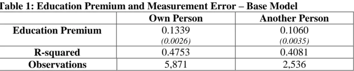
(7) With this simple model, we can evaluate more clearly changes of the impacts of education on the earnings distribution including different proxies of family educational background one by one.. Measurement Error and Attenuation Bias. Regarding measurement error, the empirical strategy pursued is to make use of the information of who responded the PNAD questionnaire on income and education, which is available in the 2014 supplement, as a proxy for measurement error and try to provide better estimates. The idea is that the measurement error will be smaller if the individual responded the questions for himself than if it was another person. In PNAD 2014, almost half of the sample responded the questionnaires for themselves, which suggest a potential large problem often ignored in household survey analysis. We split the sample in two parts: one considering only the cases in which the own person responds his labour earnings and education and another considering only the cases in which another person in the dwelling and in some rare cases outside the household answers at least one of the questions. We will use the impacts of the identity of who answers the questionnaire on the estimated R-squared and educational premium coefficients of the regression as proxies for measurement error. Therefore, the magnitude of the measurement error can be grasped intuitively by this sample split. We start by estimating a Mincerian regression controlling for the information on the parent’s education as well age, age squared, gender, geographic region of residence and dummies for urban areas. The results presented in the table below can be seen as potential indicators of the impacts of measurement error.. Table 1: Education Premium and Measurement Error – Base Model Own Person Another Person 0.1339 0.1060 Education Premium (0.0026). (0.0035). 0.4753 0.4081 R-squared 5,871 2,536 Observations Source: Author’s calculation based on PNAD 2014 supplement microdata. Obs: The numbers in bracket are the standard errors for the estimated coefficients.. The table shows that, consistent with the effects caused by measurement error that tend to spread the variance of income, the overall R-squared of the regression for 5.
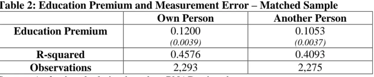
(8) those who answer the question for themselves is substantially higher than in that when another person answers. A key implication of measurement error in the Mincerian regression is the occurrence of attenuation bias in the education coefficient. As we can see, the years of schooling coefficient is also significantly greater in the sample of those who declared their own income and education. Just to make sure that the attenuation bias is statistically significant, we piled up the two samples and run a similar regression with dummies for the different sample of responders as well as these dummies interacting with the years of schooling coefficient. We have that the last coefficient turns out to be greater and statistically significant in the sample of own respondents. More precisely, the coefficient is 0.027 (with standard error 0.004), which means that the estimated education premium is approximately 2.7 per cent greater for the sample of own respondents. One final problem with the estimation above is that there may be selectivity in the generation process of different responders’ samples according to availability to answer the questionnaire, which could result in a disposability bias. For example, spouses that are mothers with small kids are more likely to be at home to answer the household survey questionnaires. Indeed, while only 46 per cent of the male responded the question about education for themselves, the corresponding number for the women is 65 per cent, which may well affect the education premium results. To deal with this selectivity bias, we used a standard logistic regression matching procedure in which we created two equal sized and more comparable samples regarding the profile of the respondents. The selection model incorporated the following variables: position in the household, if the respondent is a mother, the age of the youngest child, the type of family and individual working class.. Table 2: Education Premium and Measurement Error – Matched Sample Own Person Another Person 0.1200 0.1053 Education Premium (0.0039). 0.4576 R-squared 2,293 Observations Source: Author’s calculation based on PNAD microdata.. 6. (0.0037). 0.4093 2,275.
(9) The results using the matched sample suggest that indeed the initial comparison was probably somewhat affected by selectivity bias. The variance of the logs of income is 18.6 per cent smaller in the matched sample than in the original one. Also, the respective proportion of these inequality measures explained differs as expected for the two subsamples. In the matched sample, the difference of the R-squared of those who answered the question for themselves in comparison to the information of non-direct respondents is still significant but a little bit smaller, the same happening for the years of schooling coefficient. The difference of the R-squared of the two regressions according to the type of respondent, which was 16.47 per cent, becomes 11.8 per cent, while the difference between the years of schooling coefficient also falls from 31.53 per cent to 13.96 per cent. When we replicate the interactive model of years of schooling with the identity of the respondent, the education premium difference also falls. In sum, when we take into account both measurement error and selectivity bias issues, there is still a significant difference in the explanatory power of education in terms of individual earnings inequality and wage premiums, suggesting the presence of attenuation bias.. Omitted Variable. To start addressing the problem of omitted variable bias, we take advantage of the PNAD special supplement on intergeneration mobility, which has information on parents’ educational background. Information on parental education is rare to find in Brazilian household surveys and was available in the PNAD only for the years of 1976, 1982, 1988, 1996 and more recently 2014. Some studies have used this information to provide more precise estimates of the returns to education in Brazil. Lam and Shoeni (1993) used the PNAD 1982 supplement and found indeed that the estimated returns falls considerably when family background variables are included; Reis and Ramos (2011) find similar results using the PNAD 1996. We will focus on the 1996 and 2014 supplements, which capture the recent period of labour earnings inequality reduction in the country.. 7.
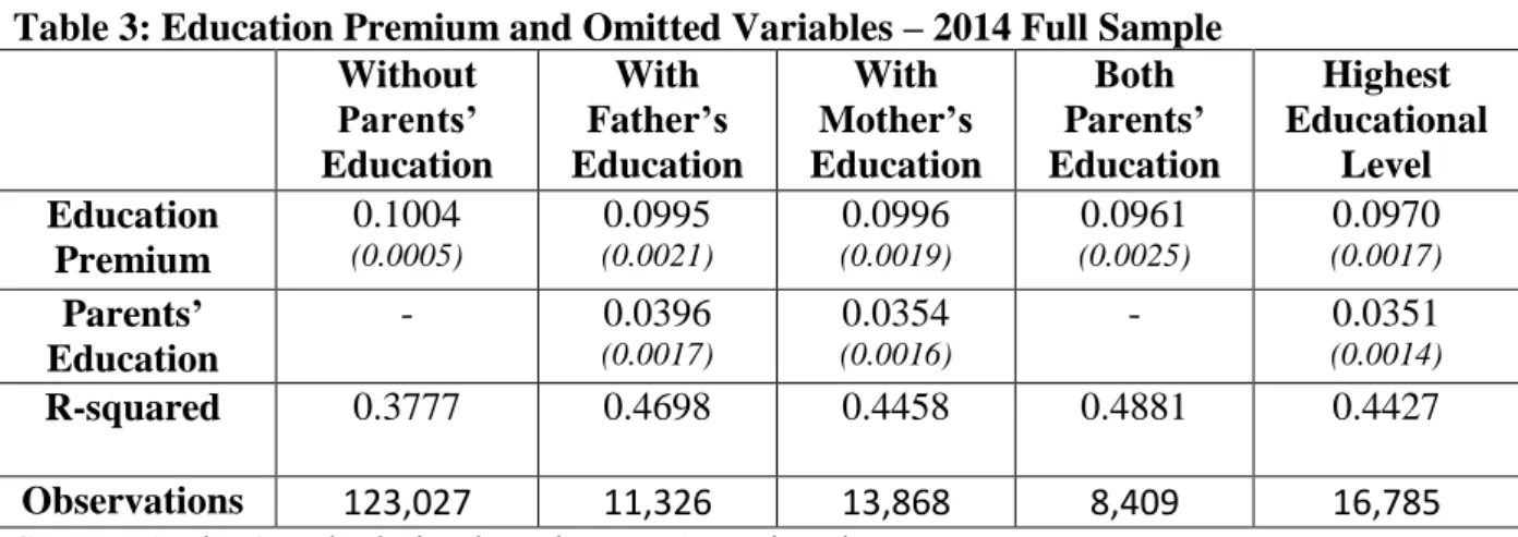
(10) Mean Years of Schooling. We start by looking at the results for 2014 using the full sample of individuals that responded the PNAD questionnaire. The results show a reduction in the wage premiums when we include the education of the parents, although the magnitude is not particularly high. We also ran a model using the highest level of education between the two parents, finding very similar results.. Table 3: Education Premium and Omitted Variables – 2014 Full Sample Without With With Both Parents’ Father’s Mother’s Parents’ Education Education Education Education 0.1004 0.0995 0.0996 0.0961 Education (0.0005) (0.0021) (0.0019) (0.0025) Premium 0.0396 0.0354 Parents’ (0.0017) (0.0016) Education 0.3777 0.4698 0.4458 0.4881 R-squared. Highest Educational Level 0.0970 (0.0017). 0.0351 (0.0014). 0.4427. Observations 123,027 11,326 13,868 8,409 16,785 Source: Author’s calculation based on PNAD microdata. Obs: The number in brackets are the standard errors for each estimated coefficient.. On the other hand, we have that the R-squared of the regressions increases significantly when we include the previously omitted variables, going from 0.3777 in the most basic specification to 0.4881 when we included both parents’ levels of education, which represents a 29 per cent increase. It is interesting to note that for the model using both levels of education, the coefficient of the education of the father is significantly larger than of the mother, 0.032 against 0.017. However, for the models using only one of the levels, the coefficients are closer: 0.0396 for the father 0.0354 for the mother and 0.0351 for the highest level. One concern is that the sample profile that responded the questions regarding parents’ education differ, as the number of observations presented in the table above may suggest. This selectivity could also bias the results found. To deal with this problem, we ran the same specifications of the model using a reduced sample containing only the individuals who responded the question for both parents. Although the results for the restricted sample point in the same direction as the ones for the full 8.
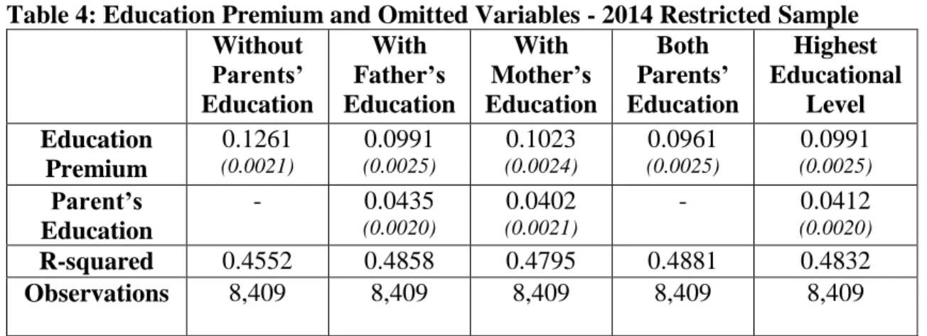
(11) sample, in the sense that there is a reduction in the wage premiums when we include information on the parents’ background, we have that the magnitudes of the reductions are much greater.. Table 4: Education Premium and Omitted Variables - 2014 Restricted Sample Without With With Both Highest Parents’ Father’s Mother’s Parents’ Educational Education Education Education Education Level 0.1261 0.0991 0.1023 0.0961 0.0991 Education (0.0021) (0.0025) (0.0024) (0.0025) (0.0025) Premium 0.0435 0.0402 0.0412 Parent’s (0.0020) (0.0021) (0.0020) Education 0.4552 0.4858 0.4795 0.4881 0.4832 R-squared 8,409 8,409 8,409 8,409 8,409 Observations Source: Author’s calculation based on PNAD microdata.. The results for the reduced sample show that the wage premiums fall significantly when we include parents’ educational background variables. While the results without including parents’ education show a wage premium of 0.1261, when we include the education of both parents it falls to 0.0961, which represents a 24 per cent reduction. Although there is also an increase in the R-squared of the regressions when we include the parents’ levels of education, the increase is smaller than for the estimations using the full sample. As for the models using the full sample, the coefficient for the education of the father is larger than for the mother when we include these two variables, 0.032 against 0.017, although the comparison between the regressions using each of the levels separately are closer, 0.0435 against 0.0402. Note that the estimated coefficients for the parent’s education using the restricted sample are always higher than for the full sample, as well as the R-squared of the regressions. The results for 1996 show that, in spite of the estimated wage premiums being higher than in 2014, there are also significant reductions in the returns to schooling when we include the previously omitted variables regarding the parents’ background. Another difference in relation to the results for 2014 is that in 1996 the coefficient of the education of the mother is larger than of the father in the model using both levels of education, 0.027 against 0.023, as well as in the models using each level separately, 0.042 against 0.038.. 9.
(12) Table 5: Education Premium and Omitted Variables - 1996 Without With With Both Parents’ Father’s Mother’s Parents’ Education Education Education Education 0.1277 0.1121 0.1118 0.1079 Education (0.0007) (0.0009) (0.0009) (0.0009) Premium 0.0383 0.0425 Parent’s (0.0012) (0.0013) Education 0.5008 0.5114 0.5118 0.5144 R-squared 55,881 55,881 55,881 55,881 Observations. Highest Educational Level 0.1116 (0.0009). 0.0363 (0.0011). 0.5109 55,881. Source: Author’s calculation based on PNAD microdata.. To assess the changes in the wage premiums from 1996 to 2014, we piled up the PNADs for the two years and ran the same specifications of the model described above with the inclusion of mean years of schooling, year dummies and a variable that captures the interaction of years of schooling with the year of 2014. Therefore, we can interpret this coefficient as the change in education returns for the period we are analysing3.. Table 6: Changes in the Educational Premium from 1996 to 2014 Without With With Both Parents’ Father’s Mother’s Parents’ Education Education Education Education Education Premium Parents Coefficient Change R-squared Observations. Highest Educational Level. 0.1277. 0.1110. 0.1136. 0.1090. 0.1105. (0.0019). (0.0020). (0.0020). (0.0020). (0.0020). -. 0.0416. 0.0403. (0.0017). (0.0018). -0.0018 *. -0.0117. -0.0125. -0.0141. -0.0114. (0.0026). (0.0026). (0.0026). (0.0026). (0.0026). 0.4940 15,912. 0.5135 15,912. 0.5106 15,912. 0.5159 15,912. 0.5122 15,912. Source: Author’s calculation based on PNAD microdata. * Not statistically significant.. 3. In 1996, all household members were assigned the question on parents’ education. In 2014, however, only one person was randomly selected. To make the two parts of the pilled samples comparable in size, we selected a random sample of PNAD 1996 with the same number of observations.. 10.
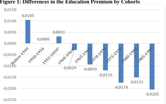
(13) The estimates point out to a reduction in the educational premium from 1996 to 2014, although the coefficient which captures this change is not statistically significant in the most basic specification without the education of the parents. However, when we include the information on the parents’ educational background, the reductions in the wage premiums for the period are higher and the coefficient becomes statistically significant. Therefore, we may be underestimating the changes if we do not consider the level of education of the parents. Our next step is to focus on a richer model with cohort dummies to see how the educational premium changes for different generations. For this purpose, we use dummies for different 5-years cohorts as well as the interaction of these dummies with years of schooling. The model with cohorts works much better when we include the previously omitted variables to assess the changes in the returns from 1996 to 2014, in the sense that all the coefficients becomes statistically significant with the expected signs. Looking directly at the cohort effects, the reduction in the educational premium has been going on for many decades and over several generations. In particular, we have that the fall in the educational premium was stronger for younger cohorts and that the relation is almost monotonic, although for the cohorts that were born between 1955 and 1959 and 1960 and 1964 the effects are not statistically different from zero.. Figure 1: Differences in the Education Premium by Cohorts 0,0150. 0,0105 0,0100 0,0031. 0,0050 0,0000. 0,0000. -0,0050 -0,0100. -0,0029. -0,0093 -0,0119. -0,0150. -0,0151 -0,0174. -0,0200. -0,0205 -0,0250. Source: Author’s calculation based on PNAD microdata. * Not statistically significant. 11.
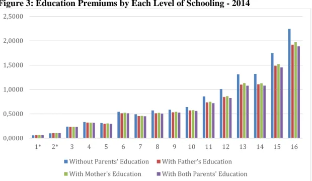
(14) Years of Schooling Distribution We also use another specification for our model in which instead of considering the mean level of schooling for the estimations of the wage education premiums, we use different dummies for each level of education, more precisely from 0 to 16 years of schooling, to assess how the wage premiums differ depending on the particular level of schooling. Following Lam and Shoeni (1993), we assess how the wage premiums change for each level of education when we add in different ways the information on parents’ background. We can see clearly that, as well as in the previous model, there are reductions in the returns to schooling when we include the information on the parents’ background. However, this disaggregated model shows that this happens not only for the average schooling but for all levels of education, the biggest reductions being observed when we include both parents’ levels of education. Also, we have that the biggest reductions happen at the higher levels of education. We did the same exercise for 1996 and found similar results.. Figure 2: Education Premiums by Each Level of Schooling - 2014 2,5000. 2,0000. 1,5000. 1,0000. 0,5000. 0,0000 1*. 2*. 3. 4. 5. 6. 7. 8. 9. 10. 11. 12. 13. 14. Without Parents' Education. With Father's Education. With Mother's Education. With Both Parents' Education. Source: Author’s calculation based on PNAD microdata.. 12. 15. 16.
(15) Figure 3: Education Premiums by Each Level of Schooling - 2014 2,5000 2,0000. 1,5000 1,0000 0,5000 0,0000 1*. 2*. 3. 4. 5. 6. 7. 8. 9. 10. 11. 12. 13. Without Parents' Education. With Father's Education. With Mother's Education. With Both Parents' Education. 14. 15. 16. 14. 16. Source: Author’s calculation based on PNAD microdata.. Figure 4: Education Premiums by Each Level of Schooling - 1996 2,5000. 2,0000. 1,5000. 1,0000. 0,5000. 0,0000 1. 2. 3. 4. 5. 6. 7. 8. 9. 10. 11. 12. 13. Without Parents' Education. With Father's Education. With Mother's Education. With Both Parents' Education. Source: Author’s calculation based on PNAD microdata.. 13.
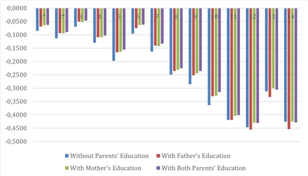
(16) Figure 5: Education Premiums by Each Level of Schooling - 1996 2,5000. 2,0000. 1,5000. 1,0000. 0,5000. 0,0000 1. 2. 3. 4. 5. 6. 7. 8. 9. 10. 11. 12. Without Parents' Education. With Father's Education. With Mother's Education. With Both Parents' Education. 13. 14. 16. Source: Author’s calculation based on PNAD microdata.. The comparison between the years of 1996 to 2014 shows reductions in the wage premiums for all levels of education in the period and for all the specifications of the model, with the bigger effects also happening at the top of the distribution.. Figure 6: Changes in the Education Premiums by Each Level of Schooling – 2014 versus 1996 0,0000. -0,0500. 1*. 2*. 3. 4. 5. 6. 7. 8. 9. 10. 11. -0,1000 -0,1500 -0,2000 -0,2500 -0,3000 -0,3500 -0,4000 -0,4500 -0,5000 Without Parents' Education. With Father's Education. With Mother's Education. With Both Parents' Education. Source: Author’s calculation based on PNAD microdata.. 14. 12. 13. 14.
(17) Quantile Regressions. To assess distributive effects in terms of income, we ran a series of quantile regressions dividing the income distribution in vintiles. We worked with two different specifications: a basic model without including the educational level of the parents and another including both parents’ levels of education. The two figures below show the distribution of the wage premiums by income vintiles for the different specifications of the model. We estimated the models for the years of 1996 and 2014. While for 1996 we have that the returns to education are reduced when we include the information on the educational background of the parents for the entire income distribution, for 2014 the results are somewhat different. While in the upper part of the distribution we also see a reduction in the wage premiums when we include the additional variables, the reverse happens in the lower part.. Figure 7: Education Premiums by Vintiles of the Income Distribution - 1996 0,14 0,13 0,12 0,11 0,1 0,09 0,08 0,05 0,1 0,15 0,2 0,25 0,3 0,35 0,4 0,45 0,5 0,55 0,6 0,65 0,7 0,75 0,8 0,85 0,9 0,95 Without Parents' Education. With Both Parents' Education. Source: Author’s calculation based on PNAD microdata.. 15.
(18) Figure 8: Education Premiums by Vintiles of the Income Distribution - 2014 0,13 0,12 0,11 0,1 0,09 0,08 0,07 0,06 0,05 0,1 0,15 0,2 0,25 0,3 0,35 0,4 0,45 0,5 0,55 0,6 0,65 0,7 0,75 0,8 0,85 0,9 0,95 Without Parents' Education. With Both Parents' Education. Source: Author’s calculation based on PNAD microdata.. When we compare the same specification across the two different years, we find that the wage premiums are smaller in 2014 in comparison with 1996 for the entire distribution, with the exception of the first vintile. On the other hand, the reductions are smaller at the basis and at the top of the income distribution and bigger at the middle of the distribution for both specifications.. Figure 9: Education Premiums by Vintiles of the Income Distribution - Without Parents’ Education 0,16 0,14 0,12 0,1 0,08 0,06 0,04 0,02 0 0,05 0,1 0,15 0,2 0,25 0,3 0,35 0,4 0,45 0,5 0,55 0,6 0,65 0,7 0,75 0,8 0,85 0,9 0,95 1996. 2014. Source: Author’s calculation based on PNAD microdata.. 16.
(19) Figure 10: Education Premiums by Vintiles of the Income Distribution – With Both Parents’ Education 0,14 0,12 0,1 0,08 0,06 0,04 0,02 0 0,05 0,1 0,15 0,2 0,25 0,3 0,35 0,4 0,45 0,5 0,55 0,6 0,65 0,7 0,75 0,8 0,85 0,9 0,95 1996. 2014. Source: Author’s calculation based on PNAD microdata.. 17.
(20) 3. Intergenerational Mobility In this section, we go beyond estimating the impacts of parental education backgrounds on wage premiums of the next generation and how it changes the estimation of the returns to education and use the information available to assess how education is transmitted across generations. Behrman, Gaviria and Székely (2001) assessed the intergenerational mobility of education in Latin America and compared with developed countries, finding significantly lower levels of mobility for the LACs, which is correlated to the high inequality levels of the region. For Brazil, they use the PNAD 1996 Supplement. Ferreira and Velloso (2003) also use the PNAD 1996 to estimate levels and effects of the transmission of education in Brazil along different dimensions, finding similar results. We provide new estimates of the level of intergenerational mobility of education in Brazil and how this relation has evolved over the period from 1996 to 2014. We make use of the same information on the parents’ education for the PNADs supplements to estimate a simple Markovian regression model of transmission of education given by: ′ 𝑆𝑖 = 𝛼 + 𝑆𝑝𝑖 𝛽 + 𝑥𝑖′ 𝛾 + 𝜀𝑖. (2). where 𝑆𝑖 is the level of schooling of the individual 𝑖, 𝑆𝑝𝑖 is a 2x1vector with the level of schooling of the parents, 𝛽 is a 2x1 vector and 𝑥𝑖 is a vector of covariates. When 𝛽 is a scalar representing the level of education of one of the parents, we have that it can be interpreted as a measure of the level of intergenerational persistence of education. Different from Behrman, Gaviria and Székely (2001) and Gasparini et al. (2017), which use the highest level of education between the two parents, we chose to focus on the level of education of the father to assess how the intergenerational transmission of education changed from 1996 to 2014 (Ferreira and Veloso 2003 follow the same strategy for 1996). To have a first idea on the educational mobility in Brazil, we estimated a transition matrix from PNAD 2014 data using the level of education of the individuals 18.
(21) and the level of education of their fathers. We restricted our analysis to individuals aged from 15 to 59 years old.. Table 7: Transition Matrix for Individuals with 15 to 59 years old - 2014 Education of the Children Elementary Middle Preschool School School High School Undergraduate Graduate 0.06 4.84 31.27 40.24 18.07 0.82. Total Education of the Father Preschool 2.41 6.84 32.91 Elementary School 0.05 5.56 30.6 Middle School 0.12 0.04 20.47 High School 0 0.2 7.25 Undergraduate 0.03 0.05 2.19 Graduate 0 0 1.32 Source: Author’s calculation based on PNAD microdata.. 33.52. 14.97. 0. 42.1 56.35 45.47 19.55 8.27. 17.64 21.6 44.25 70.66 65.96. 0.86 0.79 2.24 7.09 22.75. On the top of the distribution, we have that among fathers with an undergraduate degree, approximately 70.66 per cent of their children achieved the same level and 7.09 per cent got a graduate degree. Among fathers that completed high school, 45.47 per cent achieved the same level and 44.25 percent got an undergraduate degree. Therefore, it looks like there is some upward mobility even though the persistence is still high. The next step is to estimate equation (2) for 1996 and 2014. We controlled for age, age squared, race, geographic region of residence and dummies for urban areas. The results are presented below.. Table 8: Intergenerational Mobility in Education – 1996 and 2014 1996 2014 0.7045 0.4730 Persistence (0.0038) (0.0058) (Father’s Education Coefficient) 0.3897 0.3974 R-squared 92,978 16,284 Observations Source: Author’s calculation based on PNAD microdata.. 19.
(22) While for 1996 the estimated level of persistence was approximately 0.70, the number for 2014 is 0.47, which represents a 32.85 per cent reduction. Therefore, we have that, although the intergenerational persistence of education is still high in Brazil compared to developed countries and even other developing ones, there was a strong reduction in its level over the last two decades. To assess cohort effects, we follow a similar strategy as presented on the estimation of wage premiums. We also piled up the PNADs 1996 and 2014 and use dummies for different 5-years cohorts, as well as the interaction of these dummies with the father’s years of schooling variable to capture how the persistence changed across different generations. The results show two main findings. First, younger cohorts are more educated than older ones, as we can see by the estimated coefficients for each cohort presented in the figure below.. Figure 11: Mean Education Level by Different Cohorts 2,5000 2,0441 2,0000 1,6339 1,5000 0,9462. 1,0000. 0,7340 0,5533. 0,5000. 0,3623 0,1826 0,0000. 0,0000. -0,5000. -0,2653. Source: Author’s calculation based on PNAD microdata.. Second, we have that the fall in the intergenerational persistence of education, measured by the interaction of the education of the father with the dummies for specific cohorts, is stronger for younger cohorts, and the relation is monotonic.. 20.
(23) Figure 12: Intergenerational Mobility of Education by Different Cohorts 0,1000 0,0309. 0,0000. -0,1000. -0,2000. 0,0000. -0,0451 -0,0959 -0,1788 -0,2679. -0,3000. -0,3006 -0,3623. -0,4000. -0,4277 -0,5000. Source: Author’s calculation based on PNAD microdata.. We finish this section by estimating quantile regressions to see how the intergenerational persistence in education change along the income distribution. Again, we divided the income distribution in vintiles and estimated the level of persistence for each one considering the education of the father. The results for 1996 show that the persistence is smaller at the bottom part of the income distribution and increases as we move to the top of the distribution, reaching a maximum level of 0.81 for the 70th percentile. Then, it starts to fall until it reaches in the 95th percentile the same level of persistence as in the 10th percentile.. 21.
(24) Figure 13: Intergenerational Mobility of Education by Vintiles of the Income Distribution - 1996 0,9 0,8 0,7 0,6 0,5 0,4 0,3 0,2 0,1 0 0,05 0,1 0,15 0,2 0,25 0,3 0,35 0,4 0,45 0,5 0,55 0,6 0,65 0,7 0,75 0,8 0,85 0,9 0,95. Source: Author’s calculation based on PNAD microdata.. The results for 2014 are pretty different. We have that the persistence is higher at the bottom of the distribution and falls monotonically until it reaches the lowest level at the 95th percentile.. Figure 14: Intergenerational Mobility of Education by Vintiles of the Income Distribution - 2014 0,7 0,6 0,5 0,4 0,3 0,2 0,1 0. 0,05 0,1 0,15 0,2 0,25 0,3 0,35 0,4 0,45 0,5 0,55 0,6 0,65 0,7 0,75 0,8 0,85 0,9 0,95. Source: Author’s calculation based on PNAD microdata.. 22.
(25) Comparing directly the coefficients for the two years, we have that, except for the first two vintiles, the persistence is smaller for 2014 in comparison with 1996, specially at the middle and upper part of the income distribution. That is, we have stronger reductions in the intergenerational persistence of education for the richest individuals.. Figure: Changes in the Persistence of Education by Vintiles of the Income Distribution – 2014 versus 1996 0,30 0,21 0,20 0,10. 0,02. 0,00 -0,10 -0,20. 0,05 0,1 0,15 0,2 0,25 0,3 0,35 0,4 0,45 0,5 0,55 0,6 0,65 0,7 0,75 0,8 0,85 0,9 0,95 -0,05 -0,08 -0,12 -0,15 -0,18. -0,30 -0,40. -0,24. -0,30 -0,34-0,35 -0,36-0,37. -0,29. -0,37 -0,40 -0,44. -0,50. -0,50 -0,53. -0,60. Source: Author’s calculation based on PNAD microdata.. 4. Conclusions The paper has two main objectives. First, to provide new estimates of the level and evolution of the returns to education in Brazil based on a recently launched dataset that contains a rich and unique variety of characteristics which include family educational background. This information permits us to address some important econometric issues regarding omitted variable and measurement error biases. Second, we assess how parents’ education affect the educational level of their children and how the intergenerational mobility of education has evolved over the last years.. 23.
(26) Regarding measurement error, the empirical strategy is to make use of the information of who responded the PNAD questionnaire but controlling for availability biases. We find evidence of attenuation bias which reduces mean returns from education between 14 per cent and 31.5 per cent. On the other hand, the omitting parents’ education information also accounting for selectivity issues reduces the premium estimates by 24 percent.. Perhaps more importantly than the cross sectional estimates for 2014 cited above is the possibility of comparing omitted bias impacts across a period of sharp earnings inequality fall observed between 1996 and 2014. The fall of education premium turns out to be heavily underestimated when we do not take into account family background. The highest fall of returns occurred in intermediary levels of education and income. In the second part of the paper we assess how parents’ education affect the educational outcomes of their children and how the intergenerational mobility of education has evolved over the last years. We find a reduction on the ntergenerational persistence of education from 0.7 to 0.47 between 1996 and 2014. Comparing directly the coefficients for the two years, we have that, except for the first two vintiles, the persistence is smaller for 2014 in comparison with 1996, specially at the middle and upper part of the income distribution. That is, we have stronger reductions in the intergenerational persistence of education for the richest individuals.. Finally, cohort effects regarding intergenerational mobility also show that the fall in the persistence of education is also stronger for younger cohorts, which coincides with the fall of education premiums.. 24.
(27) References Behrman, J., A. Gaviria and M. Székely (2001). ‘Intergenerational Mobility in Latin America’. Working Paper 452. Washigton, DC: Inter-American Development Bank, Research Department. Card, D. (2001). ‘Estimating the Return to Schooling: Progress on Some Persistent Econometric Problems’. Econometrica, 69 (5): 1127-1160. Chetty, R., D. Grusky, M. Hell, N. Henderson, R. Manduca and J. Narang. ‘The Fading American Dream: Trends in Absolute Income Mobility Since 1940’. Science, 356 (6336): 398-406. Ferreira, S., and F. Velloso (2003). ‘Mobilidade Intergeracional de Educação no Brasil’. Pesquisa e Planejamento Econômico, 33 (3): 481-513. Lam, D., and R. Schoeni (1993). ‘Effect of Family Background on Earnings and Returns to Schooling: Evidence from Brazil’. Journal of Political Economy, 101 (4): 710-740. Lam, D., A. Finn and M. Leibbrandt (2015). ‘Schooling Inequality, Returns to Schooling, and Earnings Inequality’. Working Paper 2015/050. Helsinki: UNUWIDER. Lemieux, T. (2006). ‘The Mincer Equation Thirty Years After Schooling, Experience and Earnings’. In S. Grossbard (ed.), Jacob Mincer, A Pioneer of Modern Labor Economics. Springer. Mincer, J. (1974). Schooling, Experience and Earnings. New York, NY: National Bureau of Economic Research. Neidhöfer, G., J. Serrano and L. Gasparini (2017). ‘Educational Inequality and Intergenerational Mobility in Latin America: A New Database’. Discussion Paper 2017/20. Berlin: Free University Berlin, School of Business and Economics. Reis, M., and L. Ramos (2011). ‘Escolaridade dos Pais, Desempenho no Mercado de Trabalho e Desigualdade de Rendimentos’. Revista Brasileira de Economia, 65 (2): 177-205.. 25.
(28)
Imagem
+7


Documentos relacionados