Determinants of adherence to breast cancer screening in primary health care

(1)

i

2016

UNIVERSIDADE DE LISBOA FACULDADE DE CIÊNCIAS

DEPARTAMENTO DE ESTATÍSTICA E INVESTIGAÇÃO OPERACIONAL

Determinants of adherence to breast cancer screening in

primary health care

Mestrado em Bioestatística

Ana Catarina da Costa Antunes dos Santos Sousa

Trabalho de Projeto orientado por:

Prof.ª Doutora Maria Helena Mouriño Silva Nunes (FCUL) Mestre Paulo Jorge de Morais Zamith Nicola (IMPSP)

(2)

“Persistence is the road to accomplishment.”

(3)

iii

ACKNOWLEDGMENTS

I would like to briefly thank all of those who contributed throughout my thesis journey:

Helena Mouriño – my supervisor –,

for all the strength, for all the support, for all the share and of course, for always being on my side.

Duarte Tavares,

for all the work hours, all the discussions, ideas and of course, all the support and help.

Unit of Epidemiology – Institute of Preventive Medicine and Public Health,

for your support and for allowing me to work on this project. A special thank you for Paulo Nicola for all the help and support.

Alastair Gilhooley,

a really big thank you for being much more than a boss.

All my family,

for all the support specially to my parents – Adelaide & António Sousa. Without you and without your unconditional support and persistency this thesis would not have been possible.

And last but not least, to you – Sandro Leitão –,

thank you for all your support, for always being there for me and for always making me fight and not letting me give up! You know…

(4)

Cancer is a major cause of suffering and death in the European Union. Every year around 3.2 million Europeans are diagnosed with cancer. In women, every year, there is about 331,000 cases and 90,000 deaths due to breast cancer. A burden that is expected to grow even further due to demographic trends in Europe.

But with regular and systematic examinations, using evidence-based screening tests followed by appropriate treatment, it is possible to reduce cancer mortality and improve the quality of life for ones that are suffering from cancer by detecting cancer at earlier stages, when it is more responsive to less aggressive treatment.

In December 2003, the European Council unanimously adopted a set of cancer screening fundamental principles as best practice in early detection of cancer. This Council recommended to all member states that they should screen for breast cancer every woman aged between 50 and 69 years old.

Although in Portugal, screening started in the 90’s due to a pilot program where it was said that all women between 45 and 69 years old should be screened it was only in 2003 due to the European Council guideline that Portugal adopted screening with a mammogram on a biennial basis for women between 50 and 69 years old.

Mammogram screening is the only screening method that has proven to be effective. It can reduce breast cancer mortality by 20 – 30% in woman over 50 years old in high-income countries (when the screening coverage is over 70%) and is has also been associated with less disabling treatments and better quality of life after treatment.

The present work was developed in partnership with the Unidade de Epidemiologia do

Instituto de Medicina Preventiva e de Saúde Pública, Faculdade de Medicina da Universidade de Lisboa, where the main goal is to identify the profile of women who have a

longer screening delay between consecutive mammograms in primary health care units. To study the screening delay it used the Prentice-Williams-Peterson (PWP), an extension to the Cox regression model.

(5)

v From the initial population (n=41,361) 1,926 women were included. All the significant variables prove to have a protective impact on the screening delay. Women who uses hormonal contraception have an 8.5% decrease on the delay when comparing with women who do not use hormonal contraception. Women with BMI in [25 ; 30[ do screening mammograms 13.5% times with less delay when comparing to women with “normal” BMI ([18.5 ; 25[).While women with BMI ≥ 30 do screening mammograms 24.7% with less delay when comparing to women with “normal” BMI ([18.5 ; 25[).

Keywords: Breast Neoplasms, Early Detection of Cancer, Survival Analysis, Cox Regression Model

(6)

As doenças oncológicas são um dos principais problemas a nível mundial, sendo a segunda principal causa de morte em Portugal apenas atrás das doenças do aparelho circulatório.

O cancro foi a segunda causa de morte na União Europeia em 2006, seguindo as doenças cardiovasculares e tendo sido responsável por cerca de duas em cada dez mortes nas mulheres (23%) e três em cada dez nos homens (29%).

Apenas no ano de 2005 estima-se que tenham sido perdidos mais de 17 milhões de anos vida ajustados pelas incapacidades devido ao cancro na região europeia da Organização Mundial de Saúde. Segundo as estimativas da Organização Mundial de Saúde os novos casos de cancro no mundo aumentaram em 2012 e as projeções antecipam um aumento considerável para 19,3 milhões de novos casos por ano até 2025.

Devido ao envelhecimento da população espera-se que este número aumente se não forem tomadas medidas.

Os cancros da mama, colo do útero e colorretal são uma causa importante de morbilidade e mortalidade na União Europeia. Nas mulheres estes três cancros são responsáveis por cerca de um em cada dois (47%) novos casos de cancro e por uma em cada três (32%) mortes por cancro ao passo que nos homens o carcinoma colo-rectal é responsável por cerca de um em cada oito (13%) novos casos de cancro e uma em cada nove (11%) mortes o que vem aumentar a importância da implementação de programas de rastreio.

Em Portugal a situação é semelhantes com o cancro a ser a segunda cause de morte, seguindo as doenças cardiovasculares, sendo responsável por 21,1% dos óbitos.

Nas mulheres o cancro da mama é a primeira causa de morte por cancro sendo responsável por 15,9% das mortes.

Muitas vezes os médicos não conseguem explicar porque é que uma pessoa desenvolve cancro e outra não. No entanto, a investigação demonstra que determinados fatores de risco aumentam a probabilidade de uma pessoa vir a desenvolver cancro. Atualmente a tendência é de diminuição da mortalidade por cancro da mama e esta passa sobretudo pela prevenção primária. Este tipo de medida é a estratégia mais económica e eficaz no controlo do cancro e

(7)

vii ou evitados os principais fatores de risco como o tabagismo, o consumo de álcool, exposição à luz solar, radiação ionizante, determinados químicos e outras substâncias, alguns vírus e bactérias, dieta pobre, o escasso consumo de frutas e legumes, falta de atividade física ou excesso de peso. Contudo, ter um fator de risco ou vários não implica que a doença se desenvolva. Muitas mulheres com vários fatores de risco nunca desenvolveram a doença enquanto outras que desenvolveram a doença, aparentemente, não sofriam de qualquer fator de risco.

No entanto, também a prevenção secundária pode levar à diminuição da incidência de alguns tipos de cancro mediante deteção e tratamento das suas lesões precursoras.

O rastreio consiste na procura ativa de uma doença ou condição precursora de doença em indivíduos presumivelmente saudáveis em risco de desenvolver a doença, de modo a permitir terapêutica precoce.

Existem dois tipos de rastreio distintos, o populacional, no qual as pessoas em risco são convidadas a ser submetidas a rastreio, e o oportunista, que ocorre quando se aproveita para sugerir a indivíduos que recorrem aos Cuidados de Saúde Primários por outro motivo.

De um modo geral os programas de rastreio organizado são mais eficazes do que os rastreios oportunistas sendo mais económicos, mais fáceis de avaliar e, se necessário, mais fáceis de suspender.

Apesar de tudo, na União Europeia só menos de metade dos exames são efetuados no âmbito de programas populacionais que proporcional o enquadramento adequado para a implementação da garantia de qualidade exigida nos termos da recomendação do Conselho Europeu.

Rastreio é o processo seletivo para a deteção de formas precoces da doença em indivíduos assintomáticos, visando a melhoria do prognóstico da doença e a redução da mortalidade.

O rastreio oncológico pressupõe uma sequência de intervenções em tempo útil e de forma integrada desde a identificação da população alvo até à terapêutica e vigilância após tratamento para detetar o cancro com o objetivo de reduzir a mortalidade e, em alguns casos, a sua incidência.

Como o cancro é uma doença potencialmente letal o objetivo principal do rastreio oncológico é a redução da mortalidade por cancro e a avaliação da sua eficácia deve ser feita com base

(8)

importantes como a utilização de recursos de saúde e o impacto na qualidade de vida.

A evidência atual é consensual sobre a utilidade de programas de rastreio do cancro em várias áreas, incluindo, no cancro da mama.

O rastreio oncológico também acarreta várias limitações. Logo à partida baseiam-se as decisões nos benefícios populacionais em detrimento dos benefícios individuais, realizando testes num grande número de indivíduos assintomáticos, dos quais a grande maioria, não tem a doença em cause e só uma pequena parte usufruirá de benefícios pela deteção precoce do cancro.

Outro problema deve-se à acuidade dos testes, mais concretamente, à existência de falsos positivos e falsos negativos. Maioritariamente as pessoas aceitam ser rastreadas pela segurança transmitida por um resultado negativo o que tornaria este o resultado ideal. No entanto, atendendo às características do teste utilizados, perante um resultado negativo, existe sempre possibilidade de se tratar de um falso negativo e a pessoa ter a doença em causa, o que leva a uma falsa sensação de segurança e possível atraso no diagnóstico e tratamento.

Para contrariar esta limitação tendem a usar-se testes com maior sensibilidade mas existe um aumento inerente do número de falsos positivos que por sua vez causam ansiedade, rotulagem do individuo e investigação adicional desnecessária com os riscos, custos e limitações associados.

Contudo, na Europa, a mortalidade relativa ao cancro da mama reduziu 19% entre 1989 e 2006 devido à implementação das medidas de prevenção estratégica e a uma maior eficácia na terapêutica.

Uma medida de prevenção é a mamografia de rastreio e em 2003, o Conselho da União Europeia recomendou a todos os estados membros que as mulheres com idades compreendidas entre os 50 e os 69 anos deveriam efetuar rastreio de dois em dois anos.

A mamografia de rastreio provou ser o método mais eficaz. Esta é muito importante pois consegue detetar o cancro da mama mesmo antes da sensação de caroço na apalpação.

O presente estudo foi desenvolvido em parceria com a Unidade de Epidemiologia do Instituto de Medicina Preventiva e de Saúde Pública, Faculdade de Medicina da Universidade de

(9)

ix deveriam ser efetuadas de dois em dois anos, e o objetivo é identificar o perfil das mulheres que mais tempo deixam passar após a marca dos dois anos. Para traçar o perfil da mulher usaram as variáveis disponíveis e tiveram-se em conta os mais comuns fatores de risco de cancro da mama. O objetivo de identificar estas mulheres é perceber se existe algum fator comum explicativo que se possa introduzir no rastreio para que estas cumpram os dois anos.

Para modelar os tempos foi usado o modelo de Prentice-Williams-Peterson (PWP), uma extensão do Modelo de Regressão de Cox.

Da população inicial (n=41.361) 1.926 mulheres foram incluídas no estudo. Todas as variáveis significativas provaram ter um efeito protetor em relação ao tempo de não rastreio da mulher. Mulheres que usam contraceção hormonal apresentam um decréscimo no tempo de não rastreio de 8,5% quando comparadas com mulheres que não usam contraceção hormonal. Mulhers com índice de massa corporal dentro do intervalo [25;30[ fazem mamografias de rastreio 13,5% com menos atraso quando comparadas com mulheres com índice de massa corporal considerado normal, [18.5;25[. Enquanto que mulheres com índice de massa corporal superior a 30kg/m2 apresentam um tempo de não rastreio inferior em 24,7% quando comparadas com mulheres com índice de massa corporal considerado normal.

Palavras-chave: Neoplasia da Mama, Deteção Precoce de Cancro, Análise de Sobrevivência, Modelo de Regressão de Cox

(10)

INTRODUCTION ... 13 1.1 Breast cancer... 14 1.2 Risk factors ... 15 1.3 Main goal ... 17 1.4 Overview ... 18 METHODOLOGY ... 19 2.1 The project ... 20 2.2 Study population ... 20

2.2.1 Database, covariates and sampled data ... 20

2.2.2 Response variable ... 24

2.2.3 Ethical questions ... 25

2.3 Cox Regression Model ... 26

2.4 Assessment of fitting and residual analysis ... 30

2.4.1 Testing the proportional hazards ... 30

2.4.2 Residuals ... 32

2.5 Multiple events per subject ... 37

2.5.1 Symbols and notation... 37

2.5.2 Andersen-Gill Model (AG) ... 38

2.5.3 Wei-Lin-Weissfeld Model (WLW)... 39

2.5.4 Prentice-Williams-Peterson Model (PWP) ... 39

2.5.5 Comparing the models ... 40

2.6 Modelling the delay between consecutive mammograms ... 42

RESULTS ... 43

3.1 Descriptive analysis ... 44

3.2 PWP Model... 50

DISCUSSION & CONCLUSION ... 56

(11)

xi

LIST OF FIGURES

Figure 1. Mammograms’ dynamics: Multiple event times for a hypothetical woman. ... 17

Figure 2. Beginning of the study vs. woman entering the study. ... 21

Figure 3. Study design: describing the sample data for modelling purposes. ... 23

Figure 4. Percentage of women in the sample enrolled by Health Care Unit. ... 24

Figure 5. Definition of the screening delay. ... 24

Figure 6. Agency relationship. ... 25

Figure 7. Models – schematic form. ... 41

Figure 8. First screening delay for the target population and the sample. ... 46

Figure 9. Second screening delay for the target population and the sample. ... 47

Figure 10. Third screening delay for the target population and the sample. ... 47

Figure 11. Histograms for first, second and third screening delay. ... 48

Figure 12. Kaplan-Meier curves for the nominal variables in study. ... 49

Figure 13. Forest plot for hazard ratios. ... 52

Figure 14. Schoenfeld residuals graphic for Contraception. ... 53

Figure 15. Schoenfeld residuals graphic for Alcohol. ... 53

Figure 16. Schoenfeld residuals graphics for each BMI category. ... 54

(12)

Table 1. Risk factors. ... 15

Table 2. Women’s distribution by primary health care units and intervention area. ... 21

Table 3. Description of the covariates under study. ... 22

Table 4. Percentage of sampled women by each Health Care Unit. ... 23

Table 5. AG model. ... 38

Table 6. WLW model. ... 39

Table 7. PWP model. ... 40

Table 8. Representation of a subject for the three models. ... 40

Table 9. Model specific for the project. ... 42

Table 10. Target population and sampled data: socio-demographic and clinical characteristics. .. 45

Table 11. Adherence rates to mammograms screening and delayed time. ... 46

Table 12. Statistic measures, in days, for both target population and sample. ... 48

Table 13. Univariate regression estimation of the parameters. ... 50

Table 14. PWP model estimation of the parameters. ... 51

(13)

13

Chapter 1

(14)

1. INTRODUCTION

1.1 Breast cancer

Breast cancer is the most popular type of cancer within women, with approximately one million new cases every year. This cancer is also the women’s secondary cause of death in the occidental world [1].

In Portugal, it is the most frequent cancer in women with 4,500 new cases every year. This means 11 new cases per day with a daily mortality rate of 4 women with this disease [2].

The incidence of breast cancer is increasing in the developing world due to increase life expectancy, increase urbanization and adoption of western lifestyles but this increase has been counteracted in developed countries due to early diagnostic strategies and increased therapeutic effectiveness [3].

Indeed, low effective early detection programs result in a high proportion of women presenting at the latter stages of the disease, that as well as the lack of adequate diagnosis and treatment facilities are the most responsible for low survival rates [3].

Cancer occurs as a result of mutations, or abnormal changes, in the genes responsible for regulating the growth of cells and keeping them healthy – particularly in p53 genes [4]. So breast cancer is an uncontrolled growth of breast cells.

Normally, the cells replace themselves through an orderly process of cell growth – healthy new cells take over as the old ones die out. Over time, mutations can “turn on” certain genes and “turn off” others in a cell [5]. The changed cell gains the ability to keep dividing without control or order, producing more cells just like it and forming a tumour.

Breast cancer is caused by a genetic abnormality – a mistake in the genetic material. However, only 5 – 10% of cancers are due to an abnormality inherited from the parents. Instead, 85 – 90% of breast cancers are due to genetic abnormalities that happen as a result of the aging process and lifestyle in general [5].

It is possible to take steps to help the body stay as healthy as possible, these steps may have some impact in the risk of getting breast cancer but they cannot eliminate the risk.

(15)

Determinants to breast cancer screening

15 Faculdade de Ciências, Universidade de Lisboa

1.2 Risk factors

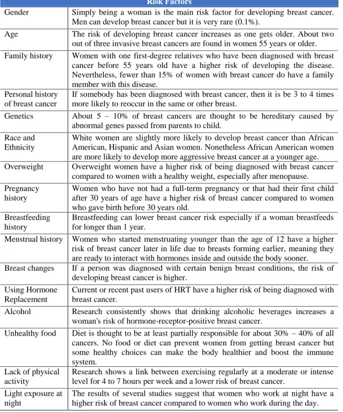
Although it is common sense that is not feasible to control whether one will have cancer, or not, we are starting to understand how it is possible to lower the risk. If it is possible to understand what to do to lower the risk then it is also possible to identify who has an increased risk. The most common risk factors are listed in Table 1 [1], [5].

Table 1. Risk factors.

Risk Factors

Gender Simply being a woman is the main risk factor for developing breast cancer. Men can develop breast cancer but it is very rare (0.1%).

Age The risk of developing breast cancer increases as one gets older. About two out of three invasive breast cancers are found in women 55 years or older. Family history Women with one first-degree relatives who have been diagnosed with breast

cancer before 55 years old have a higher risk of developing the disease. Nevertheless, fewer than 15% of women with breast cancer do have a family member with this disease.

Personal history of breast cancer

If somebody has been diagnosed with breast cancer, then it is be 3 to 4 times more likely to reoccur in the same or other breast.

Genetics About 5 – 10% of breast cancers are thought to be hereditary caused by abnormal genes passed from parents to child.

Race and Ethnicity

White women are slightly more likely to develop breast cancer than African American, Hispanic and Asian women. Nonetheless African American women are more likely to develop more aggressive breast cancer at a younger age. Overweight Overweight women have a higher risk of being diagnosed with breast cancer

compared to women with a healthy weight, especially after menopause. Pregnancy

history

Women who have not had a full-term pregnancy or that had their first child after 30 years of age have a higher risk of breast cancer compared to women who gave birth before 30 years old.

Breastfeeding history

Breastfeeding can lower breast cancer risk especially if a woman breastfeeds for longer than 1 year.

Menstrual history Women who started menstruating younger than the age of 12 have a higher risk of breast cancer later in life due to breasts forming earlier, meaning they are ready to interact with hormones inside and outside the body sooner.

Breast changes If a person was diagnosed with certain benign breast conditions, the risk of developing breast cancer is higher.

Using Hormone Replacement

Current or recent past users of HRT have a higher risk of being diagnosed with breast cancer.

Alcohol Research consistently shows that drinking alcoholic beverages increases a woman's risk of hormone-receptor-positive breast cancer.

Unhealthy food Diet is thought to be at least partially responsible for about 30% – 40% of all cancers. No food or diet can prevent women from getting breast cancer but some healthy choices can make the body healthier and boost the immune system.

Lack of physical activity

Research shows a link between exercising regularly at a moderate or intense level for 4 to 7 hours per week and a lower risk of breast cancer.

Light exposure at night

The results of several studies suggest that women who work at night have a higher risk of breast cancer compared to women who work during the day.

(16)

Some of the factors associated with breast cancer cannot be changed: gender, age, etc… but others can, by making some healthier choices. This is the case in regards to alcohol or tobacco use.

But risk factors do not tell the whole story. Having a risk factor, or even several, does not necessarily mean that the disease will trigger [1]. Most women who have one or more breast cancer risk factors never develop the disease, while many women with breast cancer have no apparent risk factors – other than being a woman and getting older. Even when a woman with risk factors develops breast cancer it is hard to know just how much these factors might have contributed to that individual case [1].

In Europe, the mortality rate due to breast cancer had a reduction of 19% between 1989 and 2006 due to the implementation of preventive strategies and a greater effectiveness on therapy [6].

One preventive strategy is screening mammograms and in 2003, the Council of the European Union recommended to all member states that they should screen every woman between 50 and 69 years of age. Despite the recommendation most of the European countries only do an opportunist screening [7].

In Portugal, the screening started in the 90’s, due to a pilot program implemented by the Region of Centro under the European Program against cancer [8]. In this program all women between 45 and 69 years of age should be screened [9]. Later, through the guideline 2003/878/CE, the European Council recommended that the screening should be done with a mammogram on a biennial basis for women between 50 and 70 years old [10].

Mammogram screening is the only screening method that has proven to be effective. It can reduce breast cancer mortality by 20 – 30% in woman over 50 years old in high-income countries when the screening coverage is over 70% [4]. Is has also been associated with less disabling treatments and better quality of life after treatment [11], [12].

The breast cancer screening has been able to reduce the mortality rate by 15% in the world and more or less 30% in Portugal. Where nine in each ten women had done screening mammograms, according to the last Portuguese National Health survey 2005/2006 [13]. A study about breast cancer showed a lower mortality in Portugal due to the increase in early detection of the disease and better access to more effective treatments [14].

(17)

According to Harris [15], observational research could potentially help to modify existing screening programs in several ways:

 By showing ways in which it is possible to improve effectiveness by changing the way screening programs are implemented;

 By finding advances in treatment or personal factors that reduces the magnitude of screening effect to the point at which the benefits no longer outweigh the harms and costs;

 By finding that the screening program grows more effective over time.

There are reasonable arguments for any of these three possible future trends in breast cancer screening programs.

1.3 Main goal

The present study is part of the project “Impact of the automatic call for breast cancer

screening in primary health care” developed by the Unidade de Epidemiologia do Instituto de Medicina Preventiva e de Saúde Pública, Faculdade de Medicina da Universidade de Lisboa.

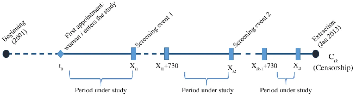
The main objective of the present work is to identify the profile of women who have a longer screening delay between consecutive mammograms in primary health care units. The time period under consideration spans from January 2001 to January 2013. Due to the dynamic nature of this study, each woman within the database might have multiple mammograms. An illustrative example of the event times under consideration is displayed in Figure 1, for a hypothetical woman.

Figure 1. Mammograms’ dynamics: Multiple event times for a hypothetical woman.

t₀ X_i1 X_i1+730 _X i2 X_ik-1+730 X_ik C ik (Censorship) Period under study Period under study Period under study

(18)

1.4 Overview

Chapter 1 gives an overview on breast cancer and risk factors. It also explains the main goal of this thesis.

Chapter 2 starts with an overview of the major project in which this thesis is included. The covariates and the response variable are also presented. Afterwards, we focus on theoretical issues about the survival analysis. More precisely, it describeds the basic Cox regression model. A brief review of the usual procedures to evaluate the proportional hazards assumption of the Cox regression model is provided. A summary of the most common residuals used in this context is also presented. The chapter ends with one of the newer areas of application of survival analysis: the use of the Cox regression model for describing multiple events per subject. It reviews three common models to accommodate the feature of the data sets: Andersen-Gill model, Wei-Lin-Weissfeld model and Prentice-Williams-Peterson model. In the present study, it applied the Prentice-Williams-Peterson model to describe mammogams’ dynamics. Therefore, it also provideds the hazard function and the partial likelihood function for modelling the delay between consecutive mammogams.

Chapter 3 summarises the most relevant results from exploratory analyses to the data sets under consideration. Then, it applies the Prentice-Williams-Peterson model to measure the impact of the covariates under consideration to the response variable, that is, screening delay between consecutive mammograms. Assessing the fit of the estimated model was also carried out.

Finally, the main conclusions and discussion on these results are given in Chapter 4. Directions for future research are also provided.

(19)

19

Chapter 2

(20)

2. METHODOLOGY

2.1 The project

The present work is part of the project “Impact of the automatic call on the breast cancer

screening in primary health care”, which is an observational retrospective longitudinal cohort

study of the primary health care units users in the larger and most populated region of Portugal – the area of Lisboa e Vale do Tejo. The major goal of the main project was to determine the effectiveness and clinical pathways on breast cancer screening performed in the primary care settings. The aim was to evaluate the impact of screening program in a global perspective, considering all stages, from the invitation process, to the screening, detection, referencing, diagnosis, treatment, follow-up and defined outcomes. This is because a screening program is much more than applying a screening technique to a vulnerable population.

This study aims at identifying the factors that lead to screening delay between mammograms. The time period under analysis spans from January 2001 to January 2013. It is worth stressing that there can be some biases, due to the institutional incentive for mammograms screening.

2.2 Study population

2.2.1 Database, covariates and sampled data

On 8th January 2013 individual clinical data was extracted from 10 primary health care units with Medicine One®, which is the software for the electronic medical records used by the doctors.

This extraction allowed having information regarding socio-demographic, clinical and comorbidities, history of mammograms and their results, history of invitations for breast cancer screening, utilization of primary health care – frequency of appointments.

(21)

So our study considers individual data, and not institutional, regional or any other form of aggregated data. Therefore, the impact of hospitals or other institutional practices to which suspected mammograms are referenced are not systematically introduced in the study.

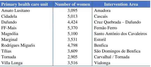
This study uses a sample of women that were followed on the primary health care units discriminated in Table 2.

Table 2. Women’s distribution by primary health care units and intervention area.

Primary health care unit Number of women Intervention Area

Amato Lusitano 3,095 Amadora

Cidadela 5,013 Cascais

Dafundo 4,424 Cruz Quebrada – Dafundo

FF-Mais 5,370 Fernão Ferro

Magnólia 5,100 Santo António dos Cavaleiros

Marginal 3,531 Estoril

Rodrigues Miguéis 4,798 Benfica

Tílias 3,609 São Domingos de Benfica

Tornada 2,905 Carvalhal / Tornada

Villa Longa 3,516 Vialonga

As it is possible to see in Table 2 the population in study is made up of 41,361 women but, of course, not every woman satisfied the criteria to be included in the study.

The first rule of inclusion, following the European Union preventive strategy, was to consider only women between 50 and 70 (exclusive) years of age. As the study began on the 1st of January 2001 all women were included, where the first doctor’s appointment via the primary health care unit on or after that date, as illustrated in Figure 2.

Figure 2. Beginning of the study vs. woman entering the study.

The second rule of inclusion was to consider women with no missing data.

The covariates focus on contraception, alcoholic habits, tobacco habits, the age as at the woman enters the study, the body mass index during the study, menarche’s age and the

(22)

number of doctor’s appointments between consecutive mammograms [3], [16], [17], [18], [19], [20], [21].

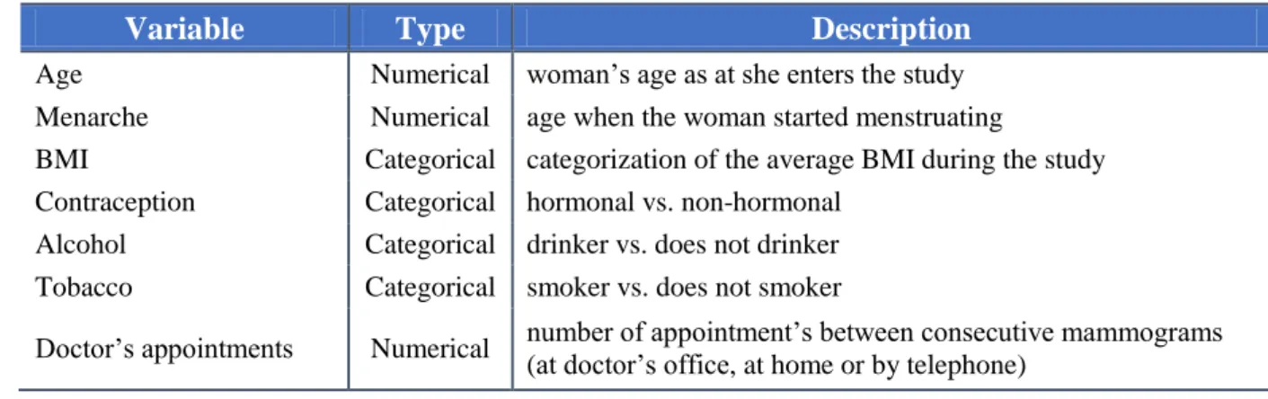
A summary of the covariates under study is presented in Table 3.

Table 3. Description of the covariates under study.

Variable Type Description

Age Numerical woman’s age as at she enters the study Menarche Numerical age when the woman started menstruating

BMI Categorical categorization of the average BMI during the study Contraception Categorical hormonal vs. non-hormonal

Alcohol Categorical drinker vs. does not drinker Tobacco Categorical smoker vs. does not smoker

Doctor’s appointments Numerical number of appointment’s between consecutive mammograms (at doctor’s office, at home or by telephone)

By restricting the age to the time at which the woman enters the study, the number of women dropped from 41,361 to 22,830.

Therefore all women were included according to their age at the moment of the screening event [15], and where no data was missing from the body mass index (BMI) and menarche’s age variables because they can be related with the appearance of cancer [21].

Right censoring occurs when a subject leaves the study because a certain event occurs, or the study ends before the event has occurred. For this particular project there were five censorship criteria [22]:

 Achieving 70 years old, as per the European Union preventive strategy and the inclusion criteria’s

 The woman’s enrolment in the primary health care unit ends, from that moment on there was no more information for that woman

 Diagnosis of breast cancer, because if cancer it is diagnosed the strategy changes  Death

(23)

And by restricting the missing data the number dropped again to 1,926 women, as represented in Figure 3.

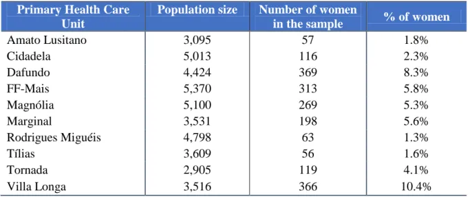
In the end, by combining all the criteria the sample is composed of 1,926 women. This final sample will be used for our study and for modeling the screening delay between consecutive mammograms. The distribution of the sampled data through the primary health care units is displayed in Table 4.

Table 4. Percentage of sampled women by each Health Care Unit.

Primary Health Care Unit

Population size Number of women

in the sample % of women

Amato Lusitano 3,095 57 1.8% Cidadela 5,013 116 2.3% Dafundo 4,424 369 8.3% FF-Mais 5,370 313 5.8% Magnólia 5,100 269 5.3% Marginal 3,531 198 5.6% Rodrigues Miguéis 4,798 63 1.3% Tílias 3,609 56 1.6% Tornada 2,905 119 4.1% Villa Longa 3,516 366 10.4%

Figure 3. Study design: describing the sample data for modelling purposes. Population: data extracted from the primary health care (n = 41,361)

Excluded 18,531 women: age out of range [50;70[

Target population: women who began the study between 50 and 70 years old (n = 22,830; 55.2%)

Excluded 20,904 women: family history of breast cancer or missing data on covariates

Sample: women with records for the variables: BMI, Menarche and with no family history of cancer (n = 1,926; 4.7%)

(24)

Figure 4. Percentage of women in the sample enrolled by Health Care Unit.

2.2.2 Response variable

As it was written above, the main goal is to understand the variables that have impact on the screening delay between consecutive mammograms.

Therefore the response variable is the delay between two consecutive mammograms, as illustrated in Figure 4. This delay begins two years and one day after the date when the mammogram took place and it ends on the previous day of the following mammogram.

Figure 5. Definition of the screening delay.

0% 2% 4% 6% 8% 10% 12% 14% 16% 18% 20% Villa Longa Tornada Tílias Rodrigues Miguéis Marginal Magnólia FF-Mais Dafundo Cidadela Amato Lusitano

Distribution of the sample by Health Care Centre

X

ij Xij+730 Xij+1

(25)

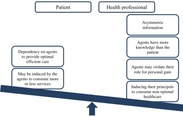
Is expected that the delay between consecutive mammograms is low as this can be impacted by the doctor’s opinion. In Health Economics this is called Agency relationship and it represents the role of a health professional in determining the patient’s best interest and acting in a fashion consistent with it, as demonstrated in Figure 5. The patient is the principal and the health professional is the agent. In health care, the situation can become complicated by virtue of the facts that the professional has an important role in determining the demand for a service as well as its supply and, also that doctors are expected – in many systems – to act not only for the patient but also for the society [23].

2.2.3 Ethical questions

From ongoing projects the Unidade de Epidemiologia already had the permission from the

Comissão de Ética da Faculdade de Medicina, the Administração Regional de Saúde de Lisboa e Vale do Tejo,IP and the Comissão Nacional de Protecção de Dados for studying the

impact of breast screening invitation in the primary health care units. This includes the ability to access to the Primary Care Electronic Medical Records and the Primary Care Referral

Patient Health professional

Asymmetric information

Agents have more knowledge than the

patient

Agents may violate their role for personal gain

Inducing their principals to consume non-optimal

healthcare May be induced by the

agents to consume more or less services Dependency on agents

to provide optimal efficient care

(26)

System, with close collaboration of the Administração Regional de Saúde de Lisboa e Vale do

Tejo.

For this project, a new submission for the Comissão de Ética da Faculdade de Medicina da

Universidade de Lisboa, Comissão de Ética para a Saúde da Administração Regional de Saúde e Vale do Tejo, IP e Comissão Nacional de Protecção de Dados was required and

approved, as well as the permission to interlink the three databases – Primary Care Electronic Medical Record, Primary Care referral system and the South Regional Cancer Registries.

2.3 Cox Regression Model

A very common issue in medical research and longitudinal studies is to model the relationship between a set of independent variables and the survival, or time to loss or censoring, outcome. The main reason why this research question cannot be addressed by straight forward multiple regression techniques, is to do with censored or incomplete event times. In these cases the Cox proportional hazard model has become the most used procedure [24], [25], [26], [27].

Considering Ti the time to the event of interest for each subject i, i1, , ,n where n is the

sample size. Thereafter we assume that the random variables T_i are independent and identically distributed with T. The survival function is defined as S t( )P T



t



..The hazard function, at time t, is the instantaneous rate of failure at time t, that is,





0 | ( ) lim . t P t T t t T t t t          

The cumulative hazard function takes the form,

0

( ) ( ) , 0. t

t  s ds t

 





Suppose that C is the censoring time for subject i, _i i1, , .n The Ci’s may be random

variables or predetermined constants. We assume that each C is independent of the _i

corresponding T_i. Let X_i min



T C_i, _i



be the follow-up time, and _i I





T_i C_i





is the status 0/1 indicator which is 1 if T_i is observed, and 0 if the observation is censored.

(27)

include a vector-valued covariates for each individual i, denoted by Zi, i1, , .n The main

goal is to estimate the hazard function or assess how the covariates affect it [24].

The Cox Regression model is the most popular procedure for modelling the time it takes for an event to occur, and it defines the hazard function for the individual i, given the covariates, as:

( ) ( ) ( ) (1)

where 0(t) is the unspecified baseline hazard function (that is, the hazard function for the

model with no covariates, Z_i  0, _i), which is a nonnegative function of time. Zi is a

p-dimensional vector of the observed covariates for subject i, and β is a px1 vector of coefficients representing the effects of the covariates [24], [28].

The event rates cannot be negative and this feature explains why the exponential function takes here a crucial role. Therefore, the Cox Regression model is a loglinear model for the covariates. In fact, expression (1) can be rewritten as ( ( )) ( ( )) . Therefore,

( ( )

( ) ) .

Also, model (1) is a semi-parametric model since the baseline hazard is non-parametric. The non-parametric term 0(t) of the Cox Regression model makes the model flexible since no

specific distribution is assumed for the baseline group.

From this model is possible to define the hazard ratio for two individuals j and k with fixed vectors of covariates, namely Zj and Zk,

( ) ( )

( )_,

which is a constant function over time. Therefore, this model is also called the Cox Proportional Hazard model.

In short, the Cox proportional hazard model can be distinguished in two parts: the first part is the underlying hazard function, called the baseline hazard, 0(t), is the hazard function for the

individual when all independent variables are equal to zero; the second part describes how the hazard function varies in response to the explanatory covariates [24].

(28)

Another advantage of the Cox Regression model is the easy interpretation of the regression parameters.

The Hazard Ratio (HR) is, by definition, the ratio of two hazard rates corresponding to the conditions described by two levels of a covariate. For illustrative purposes, suppose there is only one dichotomous covariate in the model (p=1), with levels 0 (z=0) and 1 (z=1). The HR of the individual with z=1 and the one with z=0, is given by:

( )_{( )} ( ) _{( )} ⇔ .

Hence, an individual with z=1 is exp(β) times more likely to experience the event than an individual with z=0. Therefore, the parameter β quantifies the increase (or decrease) in the log-hazard ratio for a unit increase in the covariate. If ⇒ , so the risk (or the hazard) of the event increases by (HR-1)% for an individual with z=1 compared to one with

z=0. If ⇒ , so the risk (or the hazard) of failure of the event decreases by

(1-HR)% for an individual with z=1 compared to one with z=0.

In terms of the survival at time t, ( ), it can be shown that ( ) ( ( ) ₎

.

Thus,

( ) ( ( )₎ _{( ( ))} _{( ( ))} _.

This means that if the HR=eβ is:

 Equal to 1 (that is, β=0): the covariate does not have a significant meaning in the survival time, when comparing an individual with z=1 to one with z=0;

 Higher than 1 (that is, β>0): the covariate has a nonprotective effect (i.e., lower survival) when comparing an individual with z=1 to one with z=0;

 Less than 1 (that is, β<0): the covariate has a protective effect (i.e., higher survival) when comparing an individual with z=1 to one with z=0.

A word of caution should be added here. In this study, the survival time corresponds to the time interval between two consecutive mammograms. Hence, the interpretation of the parameters of the model (and of the survival function) is the opposite of the standard interpretation. More precisely, the less the survival time the less the time interval between two

(29)

If the covariate is continuous, the ratio of the hazards for any two individuals who differ in the value of the covariate by k units is:

( )_{( )} ( ) _{( )} ( ) _{⇔ ( ) .}

Hence, k unit change in the covariate leads to the log hazard ratio of βk.

This features of the Cox proportional hazards model also applies to a p-dimensional vector of covariates: the coefficient βj, j=1,…,p, represents the increase in the log hazard ratio for a unit

increase in the corresponding covariate, zj, j=1,…,p, holding the values of the other covariates

constant.

Inference on the vector of unknown parameters, β, is based on the partial likelihood function [28], [29]. In this framework, we cannot use the full likelihood due to many nuisance parameters involved [29]. The partial likelihood depends only on the ordering of the survival times, not the actual values [24].

Suppose there are m distinct survival times, t1 < t2 < … < tm, for a sample of n observations (n

≥ m). For each time point tj there is always a group of individuals at risk, denoted by R(tj) =

Rj. Zi is the covariate vector for the individual i (i = 1,…,n).

Cox, 1975, showed that the partial likelihood is given by [29]:

(β)=∏

∑

The partial likelihood is not, in general, a likelihood in the sense of being proportional to the probability of an observed data set. However, it can be treated as likelihood for purposes of asymptotic inference [24]. In fact, Cox, 1975, [29] proved that, under very broad conditions, the usual properties of the maximum likelihood estimates and tests based on the partial likelihood still hold. More precisely, if ̂ is the maximum partial likelihood estimator of β (hereafter designated by maximum likelihood estimator) then ̂ is consistent and asymptotically Normal distributed with mean β and variance-covariance matrix given by the inverse of the observed information matrix ̂ [24]. The Newton-Raphson algorithm is used to solve the partial likelihood equation given by:

̂ _̂ _{( ̂} _{) ( ̂} _),

(30)

2.4 Assessment of fitting and residual analysis

Once the Cox model is fitted with survival data, regression diagnostics are necessary for verifying whether the statistical model fits the data appropriately or meets the proportional hazards assumption [30].

The Cox Regression model can fail in various ways. The functional form of the individual covariates may be misspecified. Furthermore, the regression coefficients may not be constant over time – violation of the proportional hazards assumption. Therefore, the proportional hazards assumption is vital to the interpretation and use of a fitted proportional hazards model.

Several ideas for residuals based on a Cox Regression model have been proposed on an ad-hoc basis, most with only limited success [24]. In the last decades, the theoretical basis for the Cox Regression model has been solidified by connecting it to the study of counting processes and Martingale theory. Therefore, the current and most successful methods are all based on counting process arguments, and in particular on the individual-specific counting process martingale that arises from this formulation [24]. Section 2.4.1 outlines the common procedures to check the proportional hazards assumption. Another graphical approach to attain this goal is based on the Schoenfeld residuals. This procedure will be postponed to Section 2.4.2.4, where we will introduce the Schoenfeld residuals. Section 2.4.2 provides a brief description of the most common residuals in the framework of the Cox regression.

2.4.1 Testing the proportional hazards

When modelling a Cox proportional hazard model a key assumption is the proportional hazards [24] – the assumption of a constant relationship between the dependent variable and the covariates which means that the hazard functions for two individuals at any point in time are proportional and independent of time. That is, the risk of an event of two individuals is the same no matter how long they survive [31].

There are several approaches for testing the proportional hazards assumption of the Cox model, ranging from simple graphical displays to sophisticated statistical tests. In this work, an overview of the most common procedures to detect nonproportionality is carried out. Section 2.4.1.1 describes a graphical procedure based on the Kaplan-Meier estimates.

(31)

2.4.1.1 Kaplan-Meier survival curves

For time-fixed variables that have a small number of levels, the simplest check of proportional hazards is to plot the survival curves for the different levels of the covariate. In Section 2.3, we showed that the survival function under the Cox model proportional hazards assumption is ( ) ( )

. Thus, ( ( ( ))) ( ( )) . Plot of the standard Kaplan-Meier estimates of survival at different levels of the covariate, and also on log-log scale, should be approximately parallel, if the proportional hazards is satisfied [24].

This method does not work well for continuous predictor or categorical predictors with many levels because the graph becomes too "cluttered".

Plot of Kaplan-Meier estimates of survival, whether transformed or not, have some limitations. Namely, the curves become sparse at longer time points; there is no reliable way to quantify how close to “parallel lines” is “close enough”; there is not a clear relationship between these plots and standard tests of proportional hazards [24].

2.4.1.2 Including time-dependent covariates in the Cox model

There are several approaches to formally test the proportional hazards assumption. Therneau and Grambsch [24] review of some of the most common methodologies. In the present work, we focus on the statistical test based on introducing time-dependent variables in the model under evaluation. For simplification purposes, we consider here that there is only one covariate in the Cox regression model.

Therneau and Grambsch [24] developed a methodology based on testing the assumption that the coefficients of the model are not time-dependent, i.e. do not change over time. This methodology relies on the creation of time-dependent covariates and then testing if the respective coefficients for interaction (first analysed separately, and then globally) are significantly different from zero.

An overview of the procedure [24]: Generate the time dependent covariates by creating interactions terms, and include them in the model. The choice of the function could be based on theoretical considerations; inspired by the smoothed residual plot, etc... Two of the most common interaction terms are the linear and log functions, leading to the following log hazard functions:

(32)

( )

( ) ( ) ( ) ( )

( ) ( ) ( )

If the time dependent covariates are significant, then those predictors do not satisfy the proportional assumption. In this case, we would need to test the null hypothesis , in either situations. If this hypothesis were rejected, then we would conclude that the proportional hazards assumption was not appropriated.

2.4.2 Residuals

In linear regression models, it is straightforward to compute residuals from the difference between the observed and the expected values for a continuous outcome variable. The lack of adequate information makes computation of regression residuals challenging in the Cox model, in turn prompting the development of a number of residual types for assessing the adequacy of the proportional hazards model [30]. Residuals may even play an important role in an attempt to assess globally goodness-of-fit.

The majority of the residuals that have been proposed in this context, mainly on an ad hoc basis, are of limited success. The current and most successful method is based on counting process arguments, and in particular on the individual-specific counting process martingale that arises from this formulation. Barlow and Prentice [32] provided the basic framework and further initial work was done by Therneau [24].

This section focus on four types of residuals that have been largely used in survival analysis:  Martingale residuals are used to determine the functional form of a covariate and also

the outliers.

 Deviance residuals are used to identify outliers.

 Score residuals are used to identify influential observations.

 Schoenfeld residuals are used to test the independence between residuals and time and hence is used to test the proportional hazards assumption.

(33)

represents the number of observed events in [0, t], for individual i; the indicator variable Yi(t)

takes the value 1 if individual i is under observation and at risk at time t, and 0 otherwise.

Consider the following counting process martingale for the individual i,

( ) ( ) ∫ ( ) ( ) (2)

where is the hazard function for individual i,

Denoting then expression (2) can be written as

Therneau and Grambsch [24] defines the martingale residuals process as,

( ) ( ) ( ) ( ) ∫ ( ) ̂ ̂ ( ) ( ) ∫ ( ) ̂ ̂ ( ), where ˆ is the maximum likelihood estimate and ˆ₀ estimates the baseline cumulative hazard (for details see [24]).

2.4.2.1 Martingale residuals

The martingale residual, for the ith individual, is defined by Mi = Ni – Ei, i=1,…,n, at the end

of the study. Formally, Mi = ̂(∞) = Ni(∞) – ̂(∞). Hereafter, we will use Mi as a shorthand

for ̂ (∞). Martingale arguments are used to show that the counting process is suitably centered and scaled and is asymptotically normally distributed.

Therneau and Grambsch [24] mentioned four properties for the martingale residuals parallel to the familiar properties from an ordinary linear model:

i. ( ) The expected value of each residuals is 0, when evaluated at the true parameter vector ;

ii. ∑ ̂ The observed residuals based on ̂ must sum to 0;

iii. ( ) The residuals computed at the true parameter vector are uncorrelated;

iv. ( ̂ ̂ ) The actual residuals are negatively correlated, as a consequence of condition (ii). ( ) i s  i1, , .n 0 ( ) ( ) ( ) , t i i i E t 



Y s  s ds N t_i( )E t_i( )M t_i( ).

(34)

Also, martingale residuals have a heavily skewed distribution with zero mean and they range in the interval (-∞,1). For censored observations, martingale residuals are negative [31].

Martingale residuals cannot fulfill all the properties that the linear model residuals do. The overall distribution of the residuals may not be helpful in the global assessment of the fit. In the linear model, the sum of squared residuals provides an overall measure of the goodness-of-fit. In the Cox Regression model when comparing models with approximately the same number of parameters, the best model do not need to have the lowest sum of squares error [24].

An additional procedure for model validation for linear models is plotting the residuals against the fitted values. A model would be accepted if a reasonable structure less horizontal band of points is observed. This is however useless for martingale residuals since the fitted values and the martingale residuals are negatively correlated.

In the linear context, the errors are assumed to be normally distributed. If the model fits the data, the residuals should have approximately the Normal distribution. The most common diagnostic plot is the Normal QQ plot, where the ordered residuals are plotted against the expected Gaussian order statistics. If the data follow a Normal distribution, then the points on the QQ plot will roughly fall along a straight line. In the Cox model context, the analogue would be the comparison of the martingale residuals to a unit exponential distribution. Therneau and Grambsch [24] shows that this procedure is a hopeless endeavour. This has to do with the fact that the semiparametric estimators of the baseline cumulative hazard rescales the martingale residuals to be roughly exponential no matter how bad the model is.

Direct assessment of the residuals, as a measure of the difference between the observed and expected values, allow us to identify individuals that are poorly fitted by the model. On the other hand, plots of the martingale residuals against individual covariates should be linear if the proportional hazards model is appropriate.

2.4.2.2 Deviance residuals

The martingale residual is highly skewed, particularly for single-event survival data, with a long right-hand tale. The deviance residual is a normalizing transform. If all covariates are time-fixed, the deviance residual is given by:

(35)

( ̂ )√ ̂ ( ̂ )

Where sign(.) is the sign function which takes the following values: 1, if its argument is positive; 0, if its argument is zero; -1, if its argument is negative. The martingale residual for the ith subject is denoted by Mi.

The martingale residuals are must more symmetrically distributed around zero than the martingale residuals.

It can be shown that the deviance residuals are formally equivalent to the Pearson residuals of the generalized linear models [24]. The deviance residuals were designed to improve on the martingale residuals for revealing individual outliers, particularly in plotting applications. In practice it has not been as useful as anticipated [24].

The sum of squared deviance residuals cannot be used to compare models because there is no guarantee that this quantity decreases with improved model fit.

The deviance residuals are often used in assessing the goodness-of-fit of a proportional hazards model. Unusual patterns of plots of deviance residuals versus individual covariates indicate that the proportional hazards model is inadequate [31].

2.4.2.3 Score residuals

The score residuals quantify, for each individual, its contribute to the partial likelihood function. Instead of a single residual for each individual, there is a separate residual for each individual and each covariate. Therefore, the score residual for the ith individual on the jth covariate is given by:

∫ [ ( ) ̅( ̂ )]

( )

where Z_ij( )s is the value of the jth covariate, for the ith subject, if this observation is still at

risk at time s; z_j

 

ˆ s is the weighted mean of the column vector of length n, the number of individuals, associated with the jth covariate over the observations still at risk at time s.

(36)

The Score residuals are useful for assessing individual influence: large values of the score residual imply large influence of the ith individual on the estimate of the parameter associated with Z_j, that is, _j. They are also useful for robust variance estimation.

The sum of the score residuals is equal to zero. Also, they are uncorrelated with one another.

2.4.2.4 Schoenfeld residuals

Tests and graphical diagnostics for the proportional hazards assumption, presented in section 2.4.1, may be based on the scaled Schoenfeld residuals. Schoenfeld proposed the first set of residuals applied with the Cox Regression model [33]. Likewise to the score residuals, instead of a single residual for each individual there is a separate residual for each individual and each covariate.

The Schoenfeld residuals are, for data without tied event times, given by:

( ) ̅( ̂ ),

where Z_{i k}_{( )}is the covariate vector of the ith subject experiencing the kth event, at the time of

that event; and z

 

ˆ t_k is the weighted mean of the covariates, for the ith subject, over those at risk at the time of the kth event.

The Schoenfeld residuals are only defined at the uncensored survival times [31]. In fact, the Schoenfeld residuals are equal to zero for all censored subjects – the majority of the packages set the value of the Schoenfeld residuals to missing for subjects whose observed survival time is censored [34].

The graphs of Schoenfeld residuals against the survival time or a covariate can be used to check the adequacy of the proportional hazards model. Unusual patterns of plots of the Schoenfeld residuals versus survival time, or individual covariates, indicate that the proportional hazards model is inadequate. Extreme departures from the main cluster indicate possible outliers or potential stability problems [31].

(37)

2.5 Multiple events per subject

The Cox Regression model was presented in section 2.3 and in that model only one event can occur for each individual. The model is simple and easy to interpret, however information about multiple and competing events is lost. There are many multivariate extensions of the survival models, namely:

 Reoccuring events

For each individual the same type of event can occur repeatedly  Competing risks

Only one event per individual yet the event can be of different types  Multi-state models

Several events and types can occur for each individual

Since this study concerns to reoccurring events for each subject, the focus will be on these models. There are several models proposed in the literature for modelling these events but it is important to distinguish between ordered and unordered data sets. Unordered datasets are not arranged in hierarchically order, e.g. family data – each family is a correlated group yet there is no constraint that one family member should die before another. Ordered data sets take in consideration the subject, i.e. each individual has the chance of experiencing the same event multiple times.

For ordered datasets, we have three approaches:  Andersen-Gill (AG) Model

 Wei, Lin and Weissefeld (WLW) Model  Prentice, Williams and Peterson (PWP) Model

Although these models have a common base there are some small differences, which will be explained next.

2.5.1 Symbols and notation

For the three models explained in detail below, it was considered the following notation, with

i=1,…n, k=1,…,K:

 Tki are the survival times for the individual i and event k

(38)

 Xki = min(Tki, Cki) is the observation time

 zki(t) is the covariate vector for the individual i and event k

 zi(t) is the covariate vector for the individual i

 Gki = Xki - Xk-1,I is the gap time with X0i = 0

 I(.) the variavel that indicates censorship with I(E) = 1 when E is true and I(E) = 0 when E is false. Then for the individual i and event k, δki = I(Tki ≤ Cki).

 ki(t) is the risk function the the individual i and event k

 β is the unknown regression parameters vector  βk is the regression parameters vector for the event k

2.5.2 Andersen-Gill Model (AG)

This model – proposed by Andersen and Gill [35] – is considered the simplest of the three models cited above but it is the one that assumes more strict assumptions [24], for example the independence between times of two events from the same individual.

Although the AG model corresponds to an extension of the Cox Regression model, it is closest in spirit to a Poisson regression by assuming that the events follow a Poisson Process dependent in time.

In this model, it is assumed each individual counting process contains independent increments – with the number of events in nonoverlapping time intervals being independent.

For the individual i, i=1, …,n, the hazard function and the partial likelihood are displayed in Table 5. Table 5. AG model. AG Model Hazard function ( ) ( ) ( ) Partial likelihood ( ) ∏ ∏ ( ( ) ∑ ∑ ( ) ( ) ) ( ) ( )

(39)

2.5.3 Wei-Lin-Weissfeld Model (WLW)

Although this model is described as treating the events in an ordered way, the WLW model treats the data as unordered competitive risks [24].

In this model, the individual is assumed to be simultaneously at risk for all events and it is at risk for each event until this event occurs. The WLW model [36] estimates the treatment effect using independent models for each event and, therefore, the relationship structure between event times does not need to be known [24].

The WLW model is the only one that allows an individual to be at risk in more than one stratum. If S is the maximum events observed for the individual than there are S stratum for the S events.

The hazard function and the partial likelihood for both models are defined in Table 6.

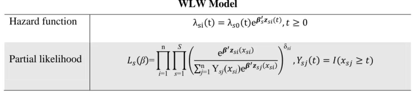
Table 6. WLW model. WLW Model Hazard function ( ) ( ) ( ) Partial likelihood (β)= ∏ ∏ ( ( ) ∑ Yn =1 ( i) ( ) ) δ_i ( ) ( ) =1 n i=1 2.5.4 Prentice-Williams-Peterson Model (PWP)

The model proposed by Prentice, Williams and Peterson is also known as the Conditional model because it assumes that the individual is not at risk of suffering the j event if the j-1 event has not happen yet [37].

There are two possible approaches depending on the processe used:

 PWP counting processes (PWP-CP) based on counting processes - the dataset follows the structure (date of enter the study; date of first event], (date of first event; date of second event], …, (date of j event; date of the last record]

 PWP gap time (PWP-GT) based on time intervals - on this after each event the time goes back to zero.

(40)

For instant t, s0(t) is the function for the time since the beginning of the study until t. The

hazard function and the partial likelihood for both models are defined in Table 7.

Table 7. PWP model. PWP-CP Hazard function ( ) ( ) ( ) Partial likelihood (β)=∏ ∏ ( ( ) ∑ ( ) ( ) ) ( ) ( ) i=1 PWP-GP Hazard function ( ) ( ) ( ) Partial likelihood (β)=∏ ∏ ( ( _{( )} ) ∑ ( ) ( ( ) ) ) ( ) ( ) i=1

2.5.5 Comparing the models

The key to represent any of the models is the structure of the dataset. Assuming a subject with events at times 10, 30 and 42, with no further follow up after the last event. For each model the intervals would be as defined in Table 8.

Table 8. Representation of a subject for the three models.

Model Interval Stratum

AG model ]0,10] 1 ]10,30[ 1 ]30,42[ 1 WLW model ]0,10] 1 ]0,30[ 2 ]0,42[ 3 PWP model ]0,10] 1 ]10,30[ 2 ]30,42[ 3

(41)

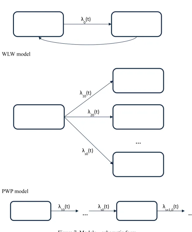
As illustrated in Figure 6, a good way of understanding the main differences is to check the schematic form for the three models. Possible transitions are represented by an arrow, with each distinct arrow corresponding to a separate stratum in the Cox Regression model [24]:

Figure 7. Models – schematic form.

For our project we will use the PWP model because, as it is possible to see in Figure 6, one woman cannot be at risk of the second screening delay if she never had the first screening delay. AG model λ 0(t) W W model λ 10(t) λ 20(t) λ s0(t)