STRESS INTENSITY FACTORS FOR NOTCHED ROUND COMPONENTS DESIGN USING FEM

STRESS INTENSITY FACTORS FOR NOTCHED ROUND

COMPONENTS DESIGN USING FEM

E.M.M.Fonseca*, F.Q.Melo**, R.A.F.Valente**

*Polytechnic Institute of Bragança – Ap. 1134, 5301-051 Bragança, Portugal. Email: [email protected] **Department of Mechanical Engineering, University of Aveiro, Portugal

Abstract

This study proposes alternative methods to estimate the stress intensity factors (SIF) of notched round components having an axial hole and subjected to an axial force or a bending moment. The method is based on analytical equations proposed by (Harris 1997) and on alternative formulation using finite element method (FEM). The objective of this work is a contribution in fracture mechanics applied to tubular systems with typical defects generated in service or a consequence of the fabrication method. Computational effort is saved with this element in the evaluation of the stress field across the section carrying the defect. Numerical examples are presented to illustrate the proposed method referring to tubular structures with different end constraints and containing a circumferential notch. The comparisons with the elastic finite element showed satisfactory results and good agreement with others references.

Key words: stress intensity factor, notch, bending moment, tubular structure.

INTRODUCTION

Tubular structures play an essential role in pipework systems, once such structure elements are part of the fluid conduction plant process in practically all chemical or energy production industries. These components frequently present geometrical discontinuities due the cross-section size variation and lacks of adhesion, as a consequence of assembling processes with welding techniques. High safety standards in design are inherent to these projects due to complex mechanical or thermal loading. When these accessories carry defects, project engineers should assess their integrity in duty. In fracture mechanics the way in which a crack is built up is not necessarily relevant; yet it is important to assess how an existing discrete crack can affect the continued operating life of the structural part carrying the defect. In a stressed structural component with defects, a crack may remain stable or propagate, eventually driving the component to fail catastrophically provided that the nominal stress field determines a critical value for the SIF associated with the crack shape and geometric parameters. The loading conditions may involve complex force system, thermal expansion effects, dynamic actions coupled with material non-homogeneity properties, where these factors represent an important role on the discrete crack evolution (Hellen 2001). Practical solutions in fracture mechanics problems are readily obtained when the finite element method is applied given its wide versatility and accuracy.

The purpose of this work has a major incidence on the evaluation of the SIF, using KI

The SIF value depends upon the crack length; the nominal stress near the crack tip and a factor considering the component geometry with deriving expressions involving some difficulty due to the characterization of the singularity at the crack tip. The stress at the tip is plastic and in elastic analysis tends to infinity (Bishop and Sherratt 2000). In structural elements where geometric singularities exist, the high level of stress there developed may determine the generation of cracks, which may propagate if the external loads are time dependent as a consequence of a fatigue phenomenon.

In this work, a finite element procedure is proposed to reduce the amount of work invested in the assessment of the components integrity eventually containing notches. This type of structural situation may arise in a stress field with a remarkable variation when subjected to bending efforts. The problem of the evaluation of the SIF along a crack existing in a pipe (Kumar et al 1985), (Parks et al 1981) is normally a task demanding some amount of computational effort, once for a reliable analysis, a highly refined finite element mesh geometry is necessary in the vicinity of the structural singularity. An economic alternative consists on the analysis of only a part of the shell containing the defect and discretized into a finite element mesh. A more elaborated finite element mesh modelling the cracked shell consists on the use of 3D FEM (Newman and Raju 1981), an option that generally involves a large number of unknowns and a less favourable consequence on the computation time; alternatively, that type of singularity may be modelled with the Line-Spring Model (LSM) (Kumar et al 1985), (Oliveira et al 1991). The concept of LSM introduced by Rice and Levy (1972) is a powerful tool when coupled with plate or shell finite element codes to assess the structural integrity of components containing cracks (Oliveira el al 1991).

This finite element appears as an attractive tool for definition of the stress field along notched surface shell element decoupled from the one-dimensional element proposed. Once defined the stress field along the edges of the component part containing notches, an approached procedure can be carried out even without a subsequent finite element analysis, using published graphical results (Harris 1997). The displacement field of the finite shell element results from the superposition of the rigid beam displacement and a complete Fourier terms development. The deformation model considered is a semi-membrane strain field, (Fonseca et al 2006). The SIF determination in a crack opening mode is function of an equation presented by (Harris 1997) from Neuber’s stress concentration factors in straight components as follows:

















c



a



  

c



t G



c a t



a

c M t a c F t c

a c

P

K_I , , 4 cos , ,

4 4 2

2 _{ }  

 

   

 



 

 (1)

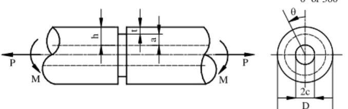
where: P represent an axial force, M the bending moment, F and G are functions of notched

geometry according figure 1.

a

t

M M

P P

2c D



h

0º or 360º

Fig. 1 - Geometric parameters for notched round component.

THE ELEMENT FORMULATION

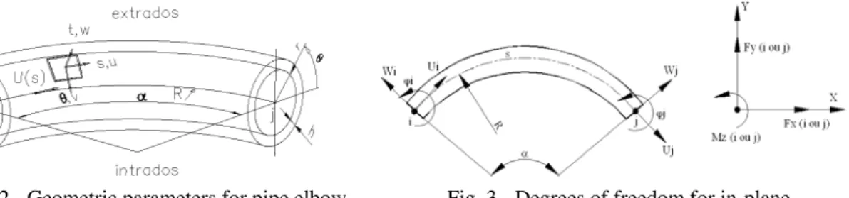
The geometric parameters considered for the piping elbow element definition are: the arc length

(s), the mean curvature radius (R), the thickness (h), the mean section radius of the pipe (r) and

the central angle (). The total number of degrees of freedom for this element is 19 for each

nodal section, being 2 translations, 1 rotation and 8 terms used in Fourier expansions. Figures 2 and 3 resume the geometric parameters and degrees of freedom for in-plane pipe elbow element.

Fig. 2 - Geometric parameters for pipe elbow. Fig. 3 - Degrees of freedom for in-plane.

The deformation field of a piping elbow element refers to membrane strains and shell curvature variations. The following assumptions, referred in (Fonseca et al 2002-2005), (Melo and Castro 1992), were considered in the present analysis: the curvature radius is assumed much larger then the section radius; a semi-membrane deformation model is adopted and neglects the bending stiffness along the longitudinal direction of the toroidal shell but considers the meridional bending resulting from ovalization.

The shell is considered thin and inextensible along the meridional direction. The shell finite

element displacement field (u, v e w), as shown figure 1, resulting from the superposition of rigid

beam displacement under mean line arc (U_{ s} , W_{ s} and



_{ s} ) and the complete Fourier expansion

for ovalization and warping terms, as show in the following equations:

 s rcos s u s,

U

u   (2)

 s sin v s,

W

v  (3)

 s cos w s,

W

w  (4)

The surface displacements along radial and meridional directions result from ovalization, in-plane, as referred by Thomson (1980) and are expressed by the following equations:

  j

n n i

n n

s a n N a n N

w 

  

      

 









2 2

, cos  cos  (5)

  j

n n i

n n

s n N

n a N

n n a

v 

  

 _     

 _









2 2

, sin  sin  (6)

The longitudinal displacement due to warping tubular section effect is calculated by the following equation, referred by (Thomson 1980):

  j

n n i

n n

s b n N b n N

u 

  

      

 









2 2

, cos  cos  (7)

The terms a_n and b_n are constants to be determined as function of developed Fourier series.

curved component is modelled. The results of these formulations were tested in different studied problems and compared with other references, (Fonseca et al 2005).

The deformation model considers that pipe undergoes a semi-membrane strain field and it is represented by the equation 8.

                                                 w v u r r s r R R s s ss 2 2 2 2 1 1 0 0 1 cos sin         

 (8)

ss

 is the longitudinal membrane strain, _s the shear strain and _ the meridional curvature

form ovalization.

The application of the virtual work principle gives finally the system of algebraic equations to be

solved. The element stiffness matrix

 

K is calculated from the matrix equation 9. A Gaussian

integration was carried out along variable s while an exact one was used along the

circumferential direction  as show in figure 4.

   

 

 

     

   

     





 

T

L s s crack T T L s s T crack element T d ds t r B D B T T d ds r B D B T K K K i f                    

 

 

        0 0 2 0 2 /        

 (9)

 

T is the transpose matrix for global system,

 

B results from the derivative of the shape

functions for the finite piping elbow element and the elasticity matrix

 

D appears with a simple

algebraic definition, dependent of the elastic modulus E, the piping elbow thickness h and

Poisson’s ratio .

 

_

_





                        2 3 2 1 12 h E 0 0 0 1 2 h E 0 0 0 1 h E

D (10)

The elasticity matrix

 

D crack is obtained replacing the value thickness h by t at equation 10.

R h x r  f _i r h re-t t re-t/2

The stress field is obtained for any position of tubular section on using Hooke’s Law along the circumferential length of the element.

 

 

 

D

 

 

  

D B

 

 (11) The membrane and bending stress are calculated for outside or inside at pipe wall using the following expressions:





      _{ }    _      2

1 2 ss s

ss t h E (12)





_     _{ }    _  _    2 1

1 2 ss

s t h E (13) ss

 is the longitudinal membrane stress and _s is the meridional bending stress due ovalization

section.

EVALUATION OF APPROXIMATION VALUES FOR SIF

The SIF determination in opening mode, equation 1, is function of an analytical equation presented by (Harris 1997) from Neuber’s stress concentration factors in straight components with a round notch for tension (P) and/or bending moment (M) for any notch position:

 P I M I

I K K

K   (14)

In the equation 1, F and G are function of notched geometry according figure 5:



, ,



0.8 4 1.08  12

                 a c c a t t a c

F and





12

08 . 1 12 . 7 8 . 0 , ,              _    a c c a t t a c

G (15)

The same equation was used for all simulations using FEM analysis for notched straight and/or curved components:



c a t



t G



c at



F t

K_I _(P)FEM    , , _(M)FEM    , , (16)

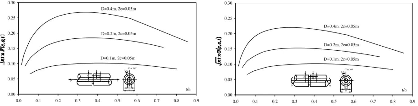
Using FEM analysis, the stress field along surface edge, gives high quality results for any notch

location. The following graphics present the results of F and G function of various notched

geometries and varying with the relation between depth notch and component wall thickness.

0.00 0.05 0.10 0.15 0.20 0.25 0.30

0.0 0.1 0.2 0.3 0.4 0.5 0.6 0.7 0.8 0.9

t/h D=0.2m, 2c=0.05m D=0.1m, 2c=0.05m D=0.4m, 2c=0.05m a t P P 2c D  h

0º or 360º

0.00 0.05 0.10 0.15 0.20 0.25 0.30

0.0 0.1 0.2 0.3 0.4 0.5 0.6 0.7 0.8 0.9

t/h D=0.2m, 2c=0.05m D=0.1m, 2c=0.05m D=0.4m, 2c=0.05m a t M M 2c D  h

0º or 360º

Fig. 5 – Several results for KI for solid notched round component in tension and in bending.

When multiplying these values by stress field the KI value is obtained for different geometries.

For a constant inside diameter the value of KI increases with thickness. The greater value is

RESULTS OF SIF

In this section, FEM stress results are presented for different curved components and the results compared with analytical stress determination for notched straight components. With the same procedure SIF determination is also determined for notched curved components using different end constraints with FEM stress analysis. The studied cases include different numerical simulations for tubular structures with different end constraints and notches surfaces. Similar

situations were verified with ANSYS finite element code using finite solid elements. All cases

are loaded with an axial force and/or a bending moment.

4.1 SIF determination in notched straight components

Figure 6 shows the geometry, the one-dimensional finite element mesh and SIF variation for different straight round geometries submitted to an axial force or a bending moment.

a

t M P 2c

D



h 0º or 360º

FEM = 7 elements

M

P 7

1

4 0

10 20 30 40 50 60 70

0 0.1 0.2 0.3 0.4 0.5 0.6 0.7 0.8 0.9 1

t/h = crack depth/thickness

KI

ANAL FEM

a) KI obtained for axial force P.

-600 -400 -200 0 200 400 600

180 210 240 270 300 330 360

Teta

KI

ANAL(t/h=0.5) FEM(t/h=0.5) FEM(t/h=0.2) FEM(t/h=0.1)

b) KI for axial force P and bending moment M.

Fig. 6 – Notched round straight component and mesh used. KI function of t/h.

Increasing the relation between crack depth and thickness component the value of KI increases

also, as show in figure 6a. When a bending moment is applied, figure 6b, the value of KI changes

along the notched section orientation angle  and increases with crack depth growth. The

numerical results agree with the analytical proposed equation 1.

4.2 Stress determination in curved components

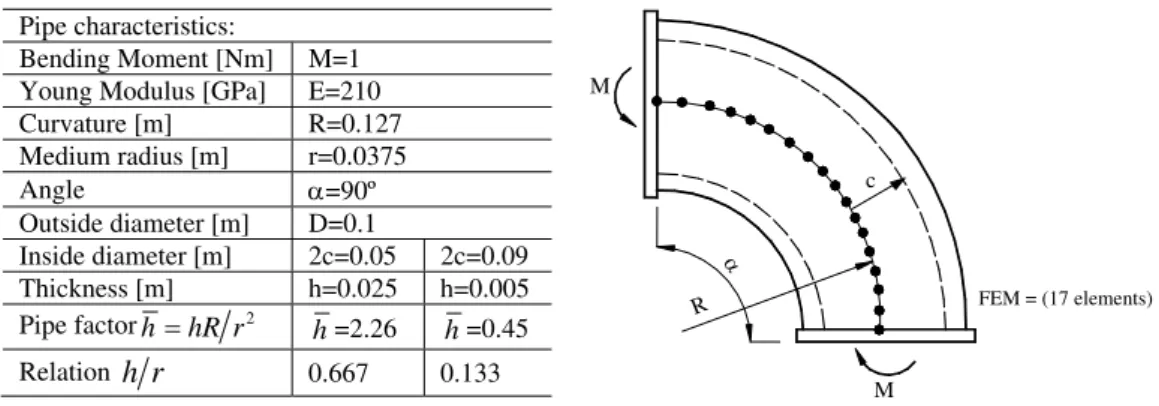
Figure 7 represents a curved component, the geometry and the mesh used in the FEM code. Results for membrane stress field are also represented at mid and end section for two different studied pipes. The curved component was analysed with different end constraints: thick, thin or without flanges. Similar stress fields were obtained with our FEM code and validated with other numerical and experimental theories as referred by (Fonseca et al 02-2005).

Pipe characteristics:

Bending Moment [Nm] M=1

Young Modulus [GPa] E=210

Curvature [m] R=0.127

Medium radius [m] r=0.0375

Angle =90º

Outside diameter [m] D=0.1

Inside diameter [m] 2c=0.05 2c=0.09

Thickness [m] h=0.025 h=0.005

Pipe factor_h_{hR r}2

h=2.26 h=0.45

Relation h r 0.667 0.133

c M

FEM = (17 elements)

M



R

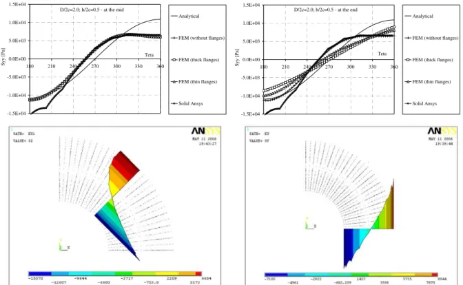
Figure 8 show the results obtained with FEM code and using ANSYS program for a pipe factor

h=2.26. Stress field is represented at mid and end zone component without notch effect as can

see. In ANSYS code a solid element was used to define the curved component mesh. The stress

results are compared with the analytical equation 14 along a section pipe considered.

D/2c=2.0; h/2c=0.5 - at the mid

-1.5E+04 -1.0E+04 -5.0E+03 0.0E+00 5.0E+03 1.0E+04 1.5E+04

180 210 240 270 300 330 360

Teta

S

yy [

P

a]

Analytical

FEM (without flanges)

FEM (thick flanges)

FEM (thin flanges)

Solid Ansys

D/2c=2.0; h/2c=0.5 - at the end

-1.5E+04 -1.0E+04 -5.0E+03 0.0E+00 5.0E+03 1.0E+04 1.5E+04

180 210 240 270 300 330 360

Teta

S

yy [

P

a]

Analytical

FEM (without flanges)

FEM (thick flanges)

FEM (thin flanges)

Solid Ansys

Fig. 8 – Stress field for different elbow end constraints at mid and end section component. h=2.26

These ANSYS results agree with those studied with FEM code when the pipe without flanges.

The ANSYS stress field was evaluated in the nodes along mid and end solid mesh section.

Figure 9 show the results obtained with FEM code for a pipe factor h=0.45. Stress field is also

represented at mid and end zone component. As shown, the stress field results depend on the pipe wall thickness and end constraints. When pipe thickness increases the stress results are similar for any type of constraint, figure 8. For thin pipes the effect of ovalization is more pronounced and stress field depend on end constrains. The analytical equation not includes this type of effect not even a finite solid element mesh.

D/2c=1.11; h/2c=0.06 - at the mid -1.5E+05

-1.0E+05 -5.0E+04 0.0E+00 5.0E+04 1.0E+05 1.5E+05

180 210 240 270 300 330 360

Teta

S

yy [

P

a]

FEM (without flanges)

FEM (thick flanges)

FEM (thin flanges)

D/2c=1.11; h/2c=0.06 - at the end -1.5E+05

-1.0E+05 -5.0E+04 0.0E+00 5.0E+04 1.0E+05 1.5E+05

180 210 240 270 300 330 360

Teta

S

yy [

P

a]

FEM (without flanges)

FEM (thick flanges)

FEM (thin flanges)

Fig. 9 – Stress field for different elbow end constraints at mid and end section component. h=0.45

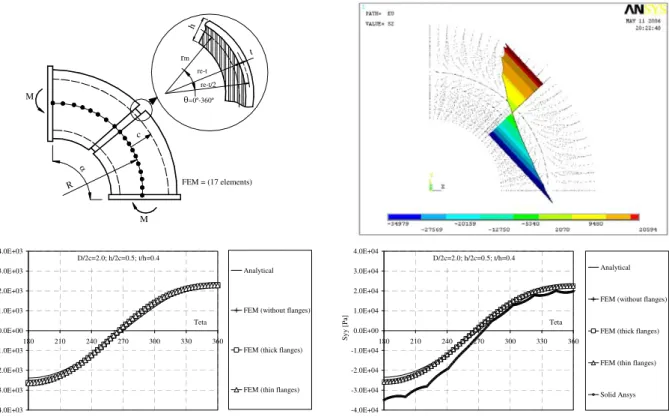
4.2.1 SIF determination in bent curved components with a notch at mid length

code and pipe characteristics are represented in figure 7. The membrane stress field and KI results

are represented at mid length of the component. KI is determined using equation 16. The results

obtained with analytical equation 1 depend on notch zone. Two different components were studied and different stress field results were obtained as shown in figures 10 and 11. The stress

field is also obtained at mid-length notch zone component using ANSYS code for a pipe factor

h=2.26. These last results agree with our FEM code results. The use of ANSYS program may be

a different representative solution but requires excessive pre-processing.

c rm

h

re-t

t

re-t/2

M _{0º-360º}

FEM = (17 elements)

M



R

D/2c=2.0; h/2c=0.5; t/h=0.4

-4.0E+03 -3.0E+03 -2.0E+03 -1.0E+03 0.0E+00 1.0E+03 2.0E+03 3.0E+03 4.0E+03

180 210 240 270 300 330 360

Teta

KI

Analytical

FEM (without flanges)

FEM (thick flanges)

FEM (thin flanges)

D/2c=2.0; h/2c=0.5; t/h=0.4

-4.0E+04 -3.0E+04 -2.0E+04 -1.0E+04 0.0E+00 1.0E+04 2.0E+04 3.0E+04 4.0E+04

180 210 240 270 300 330 360

Teta

S

yy [

P

a]

Analytical

FEM (without flanges)

FEM (thick flanges)

FEM (thin flanges)

Solid Ansys

Fig. 10 – Notched curved component. Stress field and KI calculation. h=2.26

At mid arc length component the stress results with FEM code are similar for any type of end constraints for thick piping systems, figure 10. But when the pipe is thin the results with analytical

equation shows different values as expected. The ovalization effect in KI calculation is

determinant as can be seem in figure 11. The analytical results determined with equation 16 do not include this effect and the influence of pipe wall thickness and end constraints is notorious.

D/2c=1.11; h/2c=0.06; t/h=0.5 -1.0E+04

-7.5E+03 -5.0E+03 -2.5E+03 0.0E+00 2.5E+03 5.0E+03 7.5E+03 1.0E+04

180 210 240 270 300 330 360

Teta

KI

Analytical

FEM (without flanges)

FEM (thick flanges)

FEM (thin flanges)

D/2c=1.11; h/2c=0.06; t/h=0.5 -2.0E+05

-1.5E+05 -1.0E+05 -5.0E+04 0.0E+00 5.0E+04 1.0E+05 1.5E+05 2.0E+05

180 210 240 270 300 330 360

Teta

S

yy [

P

a]

Analytical

FEM (without flanges)

FEM (thick flanges)

FEM (thin flanges)

Fig. 11 – Stress field and KI calculation. h=0.45

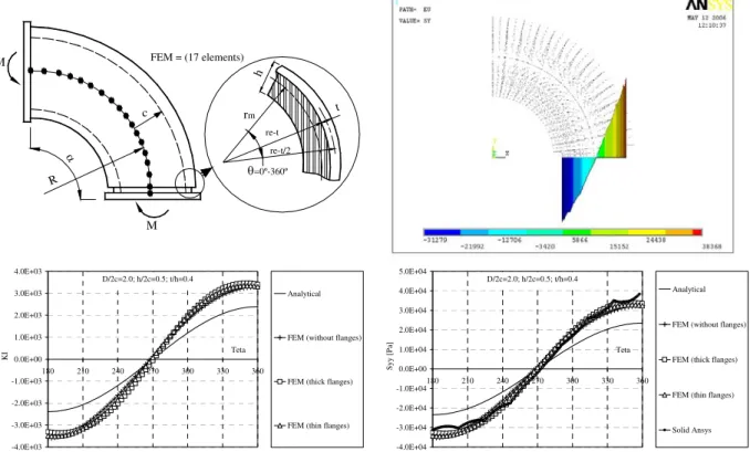
4.2.2 SIF determination in bent curved components with a notched flanged end

Figure 12 represents a component with a totally circumferential notch and the mesh used for the

constraint are also represented. The stress field is obtained near the notch zone component as

represented. ANSYS results agree with FEM code results as shown in previous analyses for a

thick pipe component.

c

M FEM = (17 elements)

M



R

rm

0º-360º

re-t/2 re-t

h

t

D/2c=2.0; h/2c=0.5; t/h=0.4

-4.0E+03 -3.0E+03 -2.0E+03 -1.0E+03 0.0E+00 1.0E+03 2.0E+03 3.0E+03 4.0E+03

180 210 240 270 300 330 360

Teta

KI

Analytical

FEM (without flanges)

FEM (thick flanges)

FEM (thin flanges)

D/2c=2.0; h/2c=0.5; t/h=0.4

-4.0E+04 -3.0E+04 -2.0E+04 -1.0E+04 0.0E+00 1.0E+04 2.0E+04 3.0E+04 4.0E+04 5.0E+04

180 210 240 270 300 330 360

Teta

S

yy [

P

a]

Analytical

FEM (without flanges)

FEM (thick flanges)

FEM (thin flanges)

Solid Ansys

Fig. 12 – Notched curved component. Stress field and KI calculation. h=2.26

Next figure represent KI and the stress evolution at notch zone for a thin pipe component.

D/2c=1.11; h/2c=0.06; t/h=0.5 -1.5E+04

-1.0E+04 -5.0E+03 0.0E+00 5.0E+03 1.0E+04 1.5E+04

180 210 240 270 300 330 360

Teta

KI

Analytical

FEM (without flanges)

FEM (thick flanges)

FEM (thin flanges)

D/2c=1.11; h/2c=0.05; t/h=0.6 -2.0E+05

-1.5E+05 -1.0E+05 -5.0E+04 0.0E+00 5.0E+04 1.0E+05 1.5E+05 2.0E+05 2.5E+05

180 210 240 270 300 330 360

Teta

Sy

y [P

a

]

Analytical

FEM (without flanges)

FEM (thick flanges)

FEM (thin flanges)

Fig. 13 – Stress field and KI calculation. h=0.45

In this case, KI value depends on end constraints and varies along section orientation angle. The

analytical results do not include the effect of bending stress due to ovalization section for thin pipes not even the type of end constraint.

The worst notched position should be near the end constraint component when compared with mid arc length position in figure 10. The presence of a notch in a pipe represents an increase in

stress field determination and therefore in KI value. All simulations presented relating this type of

conclusion. The analytical equation gives similar results when the pipe is thick, but improper results for thin pipe structures due the stress field behaviour.

CONCLUSIONS

analytical equations proposed by (Harris 1997) for straight components. The method proposed is based on the conventional shell deformation model theory adapted for tubular structures. Using FEM any type of component configuration is studied. The method is therefore a worth considering alternative to more elaborated procedures in the evaluation of the remote stress field along a notched component.

ACKNOWLEDGEMENTS

E.M.M. Fonseca gratefully acknowledges funding from the Portuguese Science and Technology Foundation; grant (SFRH/BPD/26172/2005).

REFERENCES

Harris, D.O. Stress intensity factors for hollow circumferential notched round bars. Select Papers on Crack Tip Stress Fields, R.J. Sanford Ed., SEM Classic Papers Vol.CP2, pp.185-201, (1997).

Hellen, T., How to undertake fracture mechanics analysis with finite elements, The International Association for the Engineering Analysis Community, NAFEMS Ltd. (2001).

Bishop, Dr. N. W. M., Sherratt, Dr. F., Finite element based fatigue calculations, The International Association for the Engineering Analysis Community, NAFEMS Ltd. (2000).

Kumar, V., German, M. D., Schumacher, B.I., Analysis of elastic surface cracks in cylinders using the line spring model and shell finite element method, International Journal of Pressure Vessel Technology, 107, pp.403-411, (1985).

Parks, D. M., Lockett, R. R., Brockenbrough, J. R., Stress–Intensity factors for surface – Cracked plates and cylindrical shells using line spring finite elements, Advances in Aerospace Structures and Materials, ASME AD-01, pp.279-285, (1981).

Newman, J. C., Raju, I. S., An empirical stress – intensity factor equation for the surface crack, Engineering Fracture Mechanics, 15(1-2), pp.185-192, (1981).

Oliveira, C. A. M., Melo, F. J. M. Q., Castro, P. M. S. T., The elastic analysis of arbitrary thin shells having part-through cracks using the integrated line spring and the semiloof shell elements, Engineering Fracture Mechanics, 39, pp.1027-1035, (1991).

Rice, J., Levy, N., The part-through surface crack in an elastic plate, Journal of Applied Mechanics, 39, pp.185-194, (1972).

Fonseca E.M.M., Melo F.Q., Valente R.A.F. Determination of stress intensity factors along cracked surfaces in piping elbows structures. 10th Portuguese Conference on Fracture; ISBN-972-99596-1-7, (2006).

Carpinteri A., Brighenti R., Vantadori S., Circumferentially notched pipe with an external surface crack under complex loading. International Journal of Mechanical Sciences, 45, pp.1929-1947, (2003).

Fonseca E. M. M, Melo F. J. M. Q, Oliveira C. A. M., Determination of flexibility factors on curved pipes with end restraints using a semi-analytic formulation, International Journal of Pressure Vessels and Piping, 79(12), pp.829-840 (2002).

Fonseca, E. M. M, Melo F. J. M. Q, Oliveira C. A. M., The thermal and mechanical behaviour of structural steel piping systems, International Journal of Pressure Vessels and Piping, 82(2), pp.145-153, (2005).

Melo F. J. M. Q., Castro P. M. S. T., A reduced integration Mindlin beam element for linear elastic stress analysis of curved pipes under generalized in-plane loading, Computers & Structures, 43(4), pp.787-794, (1992).