where automatic guided vehicles (AGVs) must cooperate to per-form tasks. To accomplish their goals, the AGVs must deal with localization, navigation, scheduling, and cooperation problems that must be solved autonomously. This robot competition can play an important role in education due to its inherent multidisci-plinary approach, which can motivate students to bridge different technological areas. It can also play an important role in research and development, because it is expected that its outcomes will later be transferred to real-world problems in manufacturing or service robots. By presenting a scaled-down factory shop floor, this competition creates a benchmark that can be used to compare different approaches to the challenges that arise in this kind of environment. The ability to alter the environment, in some restricted areas, can usually promote the test and evaluation of different localization mechanisms, which is not possible in other competitions. This paper presents one of the possible approaches to build a robot capable of entering this competition. It can be used as a reference to current and new teams.
Index Terms— Robotics, education, localization, navigation, prototyping.
I. INTRODUCTION
N
OWADAYS, the industry faces the need to have plants more and more flexible. For some tasks, like raw material transportation from one place of work to another, Automated Guided Vehicles (AGVs) can be used in order to allow flexible layouts. Theses transporters perform their tasks in a dynamic work environment where unexpected obstacles may appear: the workers can cross the robot path, material left behind can block the intended route and even other robots can serve as an obstacle [1]–[6]. Currently, the search for increased efficiency in a plant is a common activity and so AGVs and their deployment become a reason for an intense scientific research and pedagogical attention. This topic includes fields such as: control, localization and navigation. Observing those paradigms, the Robot@Factory competition was designed as a test platform that can be used to solve problems similar to those present in future real plants. The Robot@FactoryManuscript received October 4, 2015; revised December 11, 2015; accepted December 11, 2015. Date of publication March 2, 2016; date of current version March 3, 2016.
P. J. Costa, N. Moreira, D. Campos, and P. L. Costa are with the Department of Electrical Engineering and Computers, Faculty of Engineering, University of Porto, Porto 4099-002, Portugal (e-mail: [email protected]).
J. Gonçalves and J. Lima are with the School of Technology and Management, Polytechnic Institute of Bragança, Bragança 5301-854, Portugal. Color versions of one or more of the figures in this paper are available online at http://ieeexplore.ieee.org.
Digital Object Identifier 10.1109/RITA.2016.2518420
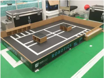
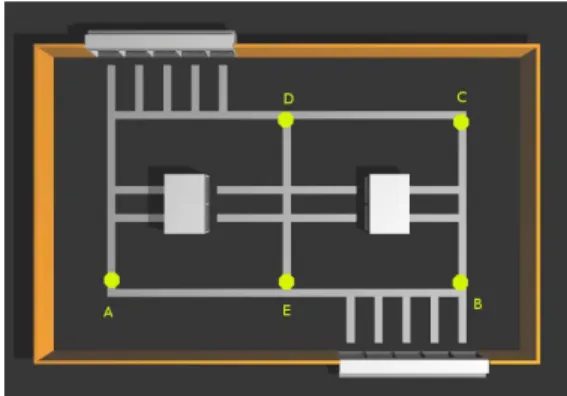
Fig. 1. Robot@Factory competition arena.
competition attempts to recreate a problem similar to the one that an autonomous robot will face during its use in a plant. This scaled plant has a supply warehouse, a final product warehouse and eight processing machines. The arena of the competition is represented in Figure 1.
The robots’ task consists in carrying the material from the supply warehouse to the machines and then to the final product warehouse. To do so, the robots must present capa-bilities which include the ability to collect, carry and put materials in the right position, locate and navigate in the given environment, as well as avoid collisions with walls, obstacles and other robots. The competition takes place in three rounds, which present challenges of increasing difficulty. This competition could help students in the transition between the junior leagues and senior ones. The SimTwo simulator provides a realistic simulation that can be used in a preliminary test of the control software. So, in order to validate all algorithms, a simulated model of the developed robot was built. By doing so, it was possible to accelerate the software development for the AGV and at the same time protect the robot hardware from the worst errors [7], [8].
The locomotion system can be built according to differ-ent topologies, for example differdiffer-ential, omnidirectional or
Ackerman. The chosen one was omnidirectional locomotion because it allows independent translation and rotation. That is not possible in the other mentioned topologies. To implement robot localization, it was used the common approach of fusing information from relative localization systems such as odometer and inertial sensors, and from an absolute local-ization system. In this case, a low-cost laser range finder
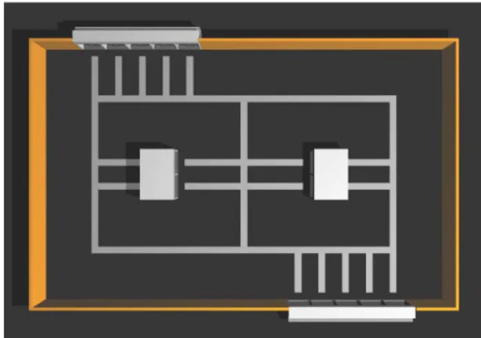
Fig. 2. Robot@Factory environment simulated inSimTwo.
was used for that purpose. One advantage of this sensor is that it can also be used to detect obstacles. Other possible approaches like following the supplied ground tracks or the use of dedicated beacons were not pursued. While following the supplied ground tracks can result in a very simple navigation system, the downside is that it constrains the set of possible trajectories. Also the need to install dedicated beacons would mean a more intrusive approach. As the underlying model is non linear it was necessary to resort to an Extended Kalman Filter. The Perfect Match algorithm [20] was used to extract the robot’s pose from the laser range finder data.
To cope with a dynamic industrial environment, where obstacle presence can be very unpredictable, a real-time path planer was implemented [9]–[14].
The paper follows this structure: initially, the SimTwo simulator is presented, then the developed robot prototype is described, next its localization system and trajectory planning are explained, and finally some results are presented and discussed.
II. SIMTWO
The SimTwo simulator already has a scenario where the arena for the Robot@Factory competition is modeled [15]. The field and all its elements are modeled in the correct scale and it is only necessary to tune the robot model. There are several sensors available like a white line detector, a LIDAR, a RGB camera or infrared distance sensors. As it can be seen in Figure 2 the 3D visualization of the simulated field looks close to the real one.
SimTwo includes a 3D rigid body engine incorporating the dynamics associated with the movement of articulated bodies. Properties like shape, mass, joints, surface friction and many others can be configured when a new scenario is modeled. Non linear effects like static friction, motors with current and voltage limitations and non linear drag can be modeled to create a realistic simulation. Normal and omnidirectional wheels are available to model different kinds of robots.
A modular environment, as it can be seen in Figure 3, lets the user visualize the 3D simulation, control its parameters,
Fig. 3. Simtwoenvironment.
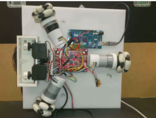
Fig. 4. Top view of the prototyped robot.
program scripts that control the robots or collect the data in real-time charts or in a built in spreadsheet.
Each scenario can be modeled using a XML based scene description language. The integrated scripting language can communicate with an external application using UDP packets. It can also be connected to external hardware over the serial port or the Ethernet version of the Modbus protocol.
III. ROBOTPROTOTYPE
A. Mechanical Project
The robot was projected and prototyped so that it could enter the Robot@Factory in a competitive way. The rules limit its size to a 45×40 cm and 35 cm high box. It was adopted an omnidirectional topology with three wheels where there are 120º between each wheel axis. This choice allows independent translation and rotation movements. The four-wheel configuration, while having some advantages, requires a mechanical suspension system. In Figures 4, 5 and 6 it is possible to see the built prototype.
B. Robot Kinematics
Fig. 5. Bottom view of the prototyped robot.
Fig. 6. Front view of the prototyped robot.
Fig. 7. Geometry of a three wheel omnidirectional robot.
velocities V1, V2 andV3, according to equation 1 [17].
⎡
⎣
Vx
Vy
ω
⎤
⎦= ⎡
⎣
a11 a12 a13 a21 a22 a23 a31 a32 a33
⎤
⎦ ⎡
⎣
V1 V2 V3
⎤
⎦ (1)
a23 = −
3si n(θ )−cos(θ )
3
a31 =a32=a33= −
1 3L
The desired global speeds V x,V yandωare related to the local speeds V,Vn andωaccording to equation 2.
⎡
⎣
V Vn
ω
⎤
⎦= ⎡
⎣
cos(θ ) si n(θ ) 0 −si n(θ ) cos(θ ) 0
0 0 1
⎤
⎦· ⎡
⎣
Vx
Vy
ω
⎤
⎦ (2)
The desired speeds for each motor can be calculated from
(V1,V2,V3). These speeds are related to (V,Vn, ω)by
equa-tion 3 [18], where L is the distance from each wheel to the robot rotation axis.
⎡
⎣
V1 V2 V3
⎤
⎦= ⎡
⎣
−si n(π/3) cos(π/3) L
0 −1 L
si n(π/3) cos(π/3) L
⎤
⎦· ⎡
⎣
V Vn
ω
⎤
⎦ (3)
Each wheel angular velocity (ω1, ω2 andω3) is related to its linear velocity by equation 4, whererri is the i-th wheel radius. Having a rotary encoder attached to each motor allows estimating the wheel angular speed by counting the number of transitions for each sample interval.
Vi =ωirri, i =1,2,3. (4)
C. Robot Hardware
The robot must be equipped with some sensors so it can perform its localization, obstacle detection and identification of the parts to be transported. Other than the mentioned encoders for each wheel the robot has a laser range finder, extracted from the robotic vacuum cleaner Neato XV-11. This laser range finder has an angular resolution of 1 degree spawning 360º, an acquisition frequency of 5 Hz and an effective range of 0.06−5 meters. As the parts that must be transported are fitted with an RGB LED that identifies the part, there are three kinds of transportable parts: one has a red LED, the other a green one and finished parts have the blue LED lit. To be able to recognize each kind of part, the robot has a USB RGB camera (aPlayStation3 Eye video camera).
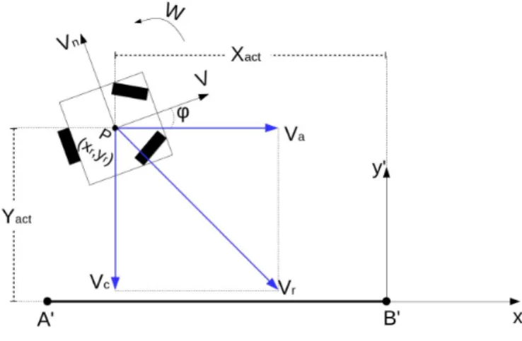
Fig. 8. Robot representation in the world and the measurement point relating to the robot.
rotation speed. This also enables the closed loop control of each motor speed.
A rotating pair of grippers is used to pick, hold and drop the parts. Two servo motors (Futaba S3003) are used to rotate each gripper.
IV. LOCALIZATION
A. Relative Localization
The robot relative localization estimate can be done through the odometry information. Performing the numerical integra-tion of the equaintegra-tions presented in III-B, the estimaintegra-tion of both position and orientation of the robot can be done. A first order approximation is exemplified in equations 5, 6 and 7, where
T is the sampling time [19].
x(k)=x(k−1)+VxT (5)
y(k)= y(k−1)+VyT (6)
θ (k)=θ (k−1)+ωT (7)
B. Absolute Localization
The absolute localization estimation uses the information gleaned from the laser range finder. From its data, the robot position and orientation are extracted using thePerfect Match
algorithm [20]. This algorithm minimizes the error between the measured and expected distances. Its implementation can be very efficient and its results can be obtained in real time.
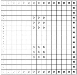
1) Map: The Perfect Match algorithm requires a local map to calculate the expected distance measures. As the Robot@Factory field map is known, it can be created offline. A matrix where each cell represents the presence or absence of an obstacle (walls, processing machines or other element present in the field) implements the known map. The chosen grid has a resolution of 1 cm.
2) Measurements Mapping: To compare the expected and the measured distances it is necessary to convert the relative distance measures to absolute coordinates. Assuming s1...sn
measurements vector, where si is the i th measure from
a full laser range finder (Figure 8) sweep, and αi is the
Fig. 9. Map example.
Fig. 10. Example of a distances map with values divided by 2.
i thmeasure angle, then the absolute position can be calculated using equation 8.
sx i
syi
=
xr
yr
+
cos(θr) si n(θr)
−si n(θr) cos(θr)
si
cos(αi)
si n(αi)
(8)
3) Error Minimization: As it was already mentioned, the
Perfect Match algorithm minimizes the error between the measured and expected distances. To speed up the error calculation, a distance map is precomputed. It is a matrix where each cell holds the distance to the closest obstacle. It can be obtained from the original map matrix by applying a Distance Transform with coefficients given by 9.
This mask performs an approximation to the Euclidean dis-tance. According to Pythagoras’ theorem, the distance between two diagonal points in a grid should be√1+1=√2 which can be approximated to 1.4142. Further adjusting this value to 1.5 allows us to, by multiplying all values by 2, have only integer distances, as can be seen in 9. There is an error of about 6% when doing this simplification.
⎡
⎣
3 2 3
2 0 2
3 2 3
⎤
⎦ (9)
estimation of the robot position is done for both x, y andθ, it is necessary to calculate the partial derivative for each of the variables. The signal of the calculated partial derivative indicates the error updating direction.
The updating value ωi j, which defines the position
dis-placement, is calculated according to the signal of the partial derivative according to equation 11.
wi j =
⎧ ⎪ ⎨
⎪ ⎩
−i j, i f sumo f gr adi ent>0
i j, i f sumo f gr adi ent<0
0, i f other values.
(11)
V. SENSORFUSION
To perform the required sensor fusion an Extended Kalman Filter was used. This algorithm can be divided in two steps, the prediction and the correction. Its state equation is represented by equation 12.
d X(t)
dt = f(X(t),u(t),t) (12)
where u(t) is a vector with the linear velocity of each wheel [23].
A. Prediction
1) State Estimate: The state estimate at each sample timetk requires the knowledge of the state intk−1 and it can
be done by the numerical integration of equations 5, 6 and 7.
2) Covariance Propagation: To calculate the covariance propagation, the linearized equations for the state transition are needed. Linearizing equation 1, around X(t) = X(tk),
u(t)=u(tk)andt =tk, leads to:
A∗(tk)=
⎡
⎣
0 0 b13
0 0 b23
0 0 0
⎤
⎦ (13)
Where:
b13 =
√
3cos(θ )+si n(θ )
3 V1−
2si n(θ )
3 V2
− √
3cos(θ )−si n(θ )
3 V3
b23 =
√
3cos(θ )+si n(θ )
3 V1+
2cos(θ )
3 V2
− √
3si n(θ )+cos(θ )
3 V3
B. Correction
1) Kalman Filter Gain: The Kalman Filter gain weights the reliability from all sources of measurement. It can be calculated by the following equation:
K(tk)=P(tk−)H(tk)T[H(tk)P(tk−)H(tk)T +R(tk)]−1 (16)
WhereR(tk)represents the measures error covariance. This
matrix Q(tk), represents the uncertainty associated with the
laser range finder measures.
As the laser range finder measures are processed by the
Perfect Match algorithm to yield the position estimate, the input matrix H(tk) is an identity matrix. So, the filter gain
equation becomes:
K(tk)=P(tk−)[P(tk−)+R(tk)]−1 (17)
2) State Estimate Update: The state estimate can be done using equation 18.
X(tk)=X(tk−)+K(tk)[z(tk)−X(tk−)] (18)
Wherez(tk)represents the calculated state that was obtained
through the Perfect Match algorithm using the laser range finder measurements.
3) Covariance Update: The last step of the Extended Kalman Filter of the calculation is the covariance update:
P(tk)= [I−K(tk)H(tk)]P(tk−1) (19)
As it was already mentioned, the matrixH(tk)is the identity
matrix, simplifying 19 to 20.
P(tk)= [I −K(tk)]P(tk−1). (20)
VI. TRAJECTORYPLANNING
After obtaining the localization it is possible to plan the robot trajectories. For this task there is a wide range of methods available. A few possibilities include simple floor line following [24] and [25] or more complex algorithms like Dijkstra’s algorithm, A∗ or Rapidly exploring random
tree [26]. The chosen approach was a modifiedA∗where there
was a tradeoff between its optimality and its computational speed. The introduced modification allows real-time results with a slight increase on the calculated path size. As the
Fig. 11. Sweep transform.
A. Map Expansion
To create a map suitable to be used with the A∗algorithm,
an initial grid with the known obstacles must be created. The cell size is a compromise between quantization error for the generated trajectory and the total grid size. A typical value, in this case, was 1 cm which creates a grid with 300 columns and 200 rows. To expand the obstacles to take into account the robot size, a few steps are necessary. The first step is to calculate the Distance Transform of the map. Then, R is calculated as the radius of the robot’s bounding circle.
The resulting grid has in every cell, where its distances are inferior to R, turned into an obstacle. The cells where the distance is R +n have its associated cost set to a non-zero value; this is a protective area. All the other cells can have associated cost set to zero. The protective exists to ensure that the optimal path keeps some distance from the obstacles.
The Distance Transform calculation uses a sweeping algorithm introduced by Borgefors in [27] Two sweepings, represented in Figure 11, are enough to calculate the Distance Transform.
1) Modification for Multiple Robots: When building the map, if other robots positions are known they can be incor-porated in the obstacles map. Then, the next steps are exactly the same.
B. A∗Algorithm
The A∗algorithm is a popular algorithm to find the shortest
path in a graph [28]. It uses an heuristic function, h(n), to estimate the remaining distance from the current node n to the target node. The estimated total cost for a path going through the current node is given by the sum of the two functions,
f(n)=g(n)+h(n), where g(h) represents the cost from the initial node to the current one. The implemented version is similar to the one defined by Costa et al. [29].
1) Construction of the Neighbor Knots: The algorithm is applied to a graph that is implicitly defined by the expanded map. Each cell is a node of the graph and its eight neighbors are implicitly connected to the central cell. The cost of tra-versing from one cell to another will be the distance between the center of each cell.
2) Structure Used for the Lists: To implement the A∗
algorithm it is usually necessary to maintain two lists: the Open List and the Closed List. The Closed List stores the nodes that were already expanded and subsequently closed. The grid can already store if one cell was already closed making the Closed List redundant. The Open List stores the
Fig. 12. Robot control after a coordinate change.
expanded nodes and it is frequently necessary to extract the best node so far. A standard ordered list has o(n) cost of inserting an element and a o(1) cost for retrieving the best one. For this problem, having in mind its typical data size, it is substantially better to use a binary heap to store the lists. With a binary heap, both the insertion and the retrieval are
o(logn)operations.
3) Heuristic: The chosen heuristic function was the Euclidian distance. This heuristic, h(n), is shown in equa-tion 21. Here, K is a gain [26], that can be used to implement a tradeoff between execution speed and the path optimality,
nx andny are the current node coordinates anddx anddy are
the target node coordinates.
h(n)=K
(nx−dx)2+(ny−dy)2. (21)
C. Navigation System
After the modified A∗ has calculated the desired path, the control system must ensure that the robot follows that trajectory. The speed controller that calculates the desired
(V,Vn, ω) is based on the presented by Conceiçã et al. in
2006 [30]. It uses the waypoints generated by the path planner to make the robot follow the line segments that connect those waypoints (Figure 12).
VII. RESULTS
A. Localization
In this section the tests done with the prototyped robot are presented and discussed. To validate the localization system, a trajectory where the robot moves through several areas of the field was chosen. This trajectory, with a total length of 3.2 m, is represented in Figure 13. It is a sequence of line segments passing through points A-B-C-D-E.
In this test, the robot starts in the position A(−1.13,−0.5,90º), then travels to point B(1.13,−0.5,0º). When the robot reaches B, it starts heading into C
Fig. 14. Comparison between the obtained localization by sensorial fusion and the one estimated by the system - test 2C.
Fig. 15. Trajectory planning with two values ofK.
Some tests were performed to tune the values for the matrices R and Q. The chosen values were R11 = R22 = R33=10E2 and Q11=Q22=10e3 and Q33=10E5.
The performed trajectory shown reveals a few moments were the noise from the localization induced small corrections preventing the robot from traveling in straight lines. A com-parison between the localization obtained by sensorial fusion and the one estimated only by the laser range finder is shown in Figure 14.
B. Trajectories
In this section the trajectory and navigation planning systems tests are presented.
The A∗algorithm generates the optimal path if the heuristic estimate does not exceed the real distance. For this problem, if the Euclidean Distance is used, that condition is met and the optimal trajectory is the result. Due to the amount of nodes that must be expanded to obtain the optimal solution, the processing time can be considerable. While not prohibitive, most of the time it prevents the real-time use of this approach. By changing the heuristic, through the introduction of a scaling factor K, the calculated path can be suboptimal but the processing time can be significantly decreased. As observed in Figure 15, the generated path for larger values of K is
Fig. 16. Trajectory planning of two robots varying Kvalues.
Fig. 17. Navigation from one warehouse to another.
Fig. 18. Navigation from one warehouse to another with two robots.
almost optimal while the processing times show an important reduction. These results are presented in table I.
To cope with the presence of other robots in the field, the map must be recalculated and the obtained trajectory is represented in Figure 16.
The navigation results, obtained in the simulator, with one or two robots are present in Figures 17 and 18.
VIII. CONCLUSION
methods that require changing the environment where the robot must operate. The modified A∗ algorithm can exhibit real-time performance so the presented navigation system can cope with a dynamic environment where the obstacles positions are changing in real-time. Also, the trajectory plan-ning system can calculate trajectories that are not confined to predefined paths. The approach was implemented and tested in a simulated environment and in a real robot, during the Robot@Factory competition. The presented approach can be used as a reference for the teams that want to enter the competition.
REFERENCES
[1] M. Pinto, A. P. Moreira, and A. Matos, “Localization of mobile robots using an extended Kalman filter in a LEGO NXT,”IEEE Trans. Educ., vol. 55, no. 1, pp. 135–144, Feb. 2012.
[2] J. Yu, K. H. Liu, and P. Luo, “A mobile RFID localization algorithm based on instantaneous frequency estimation,” inProc. 6th Int. Conf. Comput. Sci. Edu. (ICCSE), Aug. 2011, pp. 525–530.
[3] C. Ji, H. Wang, and Q. Sun, “Improved particle filter algorithm for robot localization,” inProc. 2nd Int. Conf. Edu. Technol. Comput. (ICETC), Jun. 2010, pp. V4-171–V4-174.
[4] S. C. Lee, J. S. Choi, and D.-H. Lee, “Trilateration based multi-robot localization under anchor-less outdoor environment,” inProc. 7th Int. Conf. Comput. Sci. Edu. (ICCSE), Jul. 2012, pp. 958–961.
[5] B.-S. Choi and J.-J. Lee, “The position estimation of mobile robot under dynamic environment,” inProc. 33rd Annu. Conf. IEEE Ind. Electron. Soc. (IECON), Nov. 2007, pp. 134–138.
[6] E. Prestes, “Monte Carlo localization driven by BVP,” in Proc. 33rd Annu. Conf. IEEE Ind. Electron. Soc. (IECON), Nov. 2007, pp. 2724–2729.
[7] J. Lima, J. Gonçalves, and P. J. Costa, “Modeling of a low cost laser scanner sensor,” in Proc. 11th Portuguese Conf. Autom. Control (CONTROLO), 2014, pp. 697–705.
[8] J. Gonçalves, J. Lima, and P. G. Costa, “DC motors modeling resorting to a simple setup and estimation procedure,” inProc. 11th Portuguese Conf. Autom. Control (CONTROLO), 2014, pp. 441–447.
[9] I. Randria, M. M. B. Khelifa, M. Bouchouicha, and P. Abellard, “A comparative study of six basic approaches for path planning towards an autonomous navigation,” in Proc. 33rd Annu. Conf. IEEE Ind. Electron. Soc. (IECON), Nov. 2007, pp. 2730–2735.
[10] C.-C. Tsai, H.-C. Huang, and C.-K. Chan, “Parallel elite genetic algo-rithm and its application to global path planning for autonomous robot navigation,”IEEE Trans. Ind. Electron., vol. 58, no. 10, pp. 4813–4821, Oct. 2011.
[11] N. B. Hui, “Coordinated motion planning of multiple mobile robots using potential field method,” inProc. Int. Conf. Ind. Electron., Control Robot., Dec. 2010, pp. 6–11.
[12] S. L. X. Francis, S. G. Anavatti, and M. Garratt, “Online incremental and heuristic path planning for autonomous ground vehicle,” inProc. 37th Annu. Conf. IEEE Ind. Electron. Soc. (IECON), Nov. 2011, pp. 233–239. [13] M. Engin and D. Engin, “Path planning of line follower robot,” inProc.
5th Eur. DSP Edu. Res. Conf. (EDERC), Sep. 2012, pp. 1–5. [14] H. Kim and B. K. Kim, “Online minimum-energy trajectory
plan-ning and control on a straight-line path for three-wheeled omnidi-rectional mobile robots,” IEEE Trans. Ind. Electron., vol. 61, no. 9, pp. 4771–4779, Sep. 2014.
[15] Comissão Especializada para o Festival Nacional de Robótica, Robot@Factory—Competition Rules and Technical Specifications, 2013. [16] P. J. Costa. (2014). Paco/Wiki—Main/SimTwo. [Online]. Available:
http://paginas.fe.up.pt/~paco/wiki/index.php?n=Main.SimTwo
[17] R. Siegwart, I. R. Nourbakhsh, and D. Scaramuzza, Introduction to Autonomous Mobile Robots. Cambridge, MA, USA: MIT Press, 2011. [18] H. P. Oliveira, A. J. Sousa, A. P. Moreira, and P. J. Costa, “Modeling and assessing of omni-directional robots with three and four wheels,” in
Contemporary Robotics: Challenges and Solutions. 2009, pp. 109–138. [19] J. Gonçalves,Controlo de Robots Omnidireccionais. 2005.
[20] M. Lauer, S. Lange, and M. Riedmiller, “Calculating the perfect match: An efficient and accurate approach for robot self-localization,” in RoboCup 2005: Robot Soccer World Cup IX, vol. 4020. 2005, pp. 142–153.
[21] M. Riedmiller, “Rprop-description and implementation details,” Tech. Rep., 1994, pp. 5–6.
[22] M. Riedmiller and H. Braun, “A direct adaptive method for faster backpropagation learning: The RPROP algorithm,” in Proc. IEEE Int. Conf. Neural Netw., Mar. 1993, pp. 586–591.
[23] J. Gonçalves, “Modelação e simulação realista de sistemas no domínio da robótica móvel,” Tech. Rep., 2009.
[24] M. Makrodimitris, A. Nikolakakis, and E. Papadopoulos, “Semi-autonomous color line-following educational robots: Design and implementation,” in Proc. IEEE/ASME Int. Conf. Adv. Intell. Mechatronics (AIM), Jul. 2011, pp. 1052–1057.
[25] Y. Li et al., “An improved line following optimization algo-rithm for mobile robot,” in Proc. 7th Int. Conf. Comput. Converg. Technol. (ICCCT), Dec. 2012, pp. 84–87.
[26] P. L. Costa, “Planeamento Cooperativo de Tarefas e Trajectórias em Múltiplos Robôs,” Tech. Rep., 2011.
[27] G. Borgefors, “Distance transformations in arbitrary dimensions,”
Comput. Vis., Graph., Image Process., vol. 27, no. 3, pp. 321–345, Sep. 1984.
[28] S. Russell and P. Norvig,Artificial Intelligence: A Modern Approach. Englewood Cliffs, NJ, USA: Prentice-Hall, 2009.
[29] P. J. Costa, A. P. Moreira, and P. Costa, “Real-time path planning using a modified A∗ algorithm,” in Proc. 9th Conf. Mobile Robots Competitions (ROBOTICA), May 2009, pp. 147–152.
[30] A. S. Conceição, A. P. Moreira, and P. J. Costa, “Controller optimization and modelling of an omni-directional mobile robot,” in Proc. 7th Portuguese Conf. Autom. Control, 2006, pp. 1–6.
Paulo José Costawas born in Porto, Portugal, in 1968. He received the bach-elor’s, master’s, and Ph.D. degrees in computers and electrical engineering from the University of Porto, Portugal, in 1991, 1995, and 2000, respectively. He is currently a Lecturer with the Faculty of Engineering, University of Porto, in automation, robotics, and digital systems. He is a Senior Member of the Robotics and Intelligent Systems Research Group from INESC-TEC. He participated in several mobile robot competitions, both as a proponent as well as a participant. He is one of the proponents of the Robot@Factory competition. His main research areas are modeling, localization, control, and prototyping of mobile robots.
Nuno Moreira was born in Aveiro, Portugal, in 1989. He received the master’s degree in computers and electrical engineering from the University of Porto, Portugal, in 2014, presenting a thesis entitled Localization of Autonomous Mobile Robots in an Industrial Environment. He is a member of the FeupFactory Team that participates at the Robot@Factory competition.
Daniel Camposwas born in Porto, Portugal, in 1990. He received the master’s degree in computers and electrical engineering from the University of Porto, Portugal, in 2014, presenting a thesis entitled Trajectory Planning of Multiple Robots in an Industrial Environment. He is a member of the FeupFactory Team that participates at the Robot@Factory competition.