FIELD CALIBRATIONA TOOLFOR ACOUSTIC NOISE PREDICTION:
THE CALCOM’10 DATA SET
Felisberto, P.; Jesus,S.;Martins,N.
Institute for Systems and Robotics University of Algarve 8005-139 Faro
{pfelis, sjesus, nmartins}@ualg.pt
ABSTRACT
It is widely recognized that anthropogenic noise affects the marine fauna, thus it becomes a major concern in ocean management policies. In the other hand there is an increasing demand for wave energy installations that, presumably, are an important source of noise. A noise prediction tool is of crucial importance to assess the impact of a perspective installation. Contribute for the development of such a tool is one of the objectives of the WEAM project. In this context, the CALCOM’10 sea trial took place off the south coast of Portugal, from 22 to 24 June, 2010 with the purpose of field calibration. Field calibration is a concept used to tune the parameters of an acoustic propagation model for a region of interest. The basic idea is that one can significantly reduce the uncertainty of the predictions of acoustic propagation in a region, even with scarce environmental data (bathymetric, geoacoustic), given that relevant acoustic parameters obtained by acoustic inference (i.e. acoustic inversion) are integrated in the prediction scheme. For example, this concept can be applied to the classical problem of transmission loss predictions or, as in our case, the problem of predicting the distribution of acoustic noise due to a wave energy power plant. In such applications the accuracy of bathymetric and geoacoustic parameters estimated by acoustic means is not a concern, but only the uncertainty of the predicted acoustic field. The objective of this approach is to reduce the need for extensive hydrologic and geoacoustic surveys, and reduce the influence of modelling errors, for example due to the bathymetric discretization used. Next, it is presented the experimental setup and data acquired during the sea trial as well as preliminary results of channel characterization and acoustic forward modelling.
Keywords: acoustic field calibration, equivalent acoustic model, acoustic inversion
INTRODUÇÃO
Nowadays there is an increasing demand for renewable energy sources. In this context the number of renewable energy installations in the ocean, off-shore wind mills and wave energy farms, will likely grow in the future. Such a power plant, composed by several generators, will produce considerable acoustic noise that propagates through the ocean and will affect the oceanic environment and the marine fauna to some extend. In November 2007 the project Wave Energy Acoustic Monitoring (WEAM) was initiated aiming at developing, testing and validating a monitoring system for determining underwater acoustic noise generated by wave generators and their impact in the sea fauna. Another objective of this project is to develop a methodology to predict the noise distribution on a candidate area for installation of a wave energy farm. The development of such a methodology will give rise to tools that will allow the developer/engineering team in an early phase of the project
(a) (b)
Fig. 1 - CALCOM’10 work area off the south coast of Portugal (magenta box) (a). Bathymetry map of the work area with the superimposed ship/source track (dotted line) of the events of 24th June 2010, AOB21 point
of deployment (star A1d) and recovery (star A1r), AOB22 point of deployment (square A2d), track (thick black line) and point of recovery (square A2r). The green lines over the ship/source and AOB22 tracks represent the locations of transmission and reception of probe signals (b).
to predict the influence of such an installation in the environment or decide about the optimal configuration in order to mitigate it. An initial model of noise distribution can be obtained by combining archival data, both hydrologic and seafloor, with outputs of oceanographic and acoustic modelling tools. However, this initial acoustic noise model should be refined with actual measurements in the interest area, even in case a large archival data set is available. Although, several approaches can be considered to minimize the modelling errors, for instance based on frequent sound speed profile measurements, bottom surveys and cores and more powerful modelling tools, which are costly, herein an alternative method is considered. This alternative method, named (acoustic) field calibration consists in integrating on the final acoustic noise distribution predictions, results obtained from acoustic inversions of acoustic sensitive parameters, like bathymetric and geoacoustic parameters. The idea is that, information of the environment obtained by acoustic inversions is sufficient and irreplaceable to attain an acoustic noise model of the area for the proposals considered above. The field calibration method is a low cost method when compared with other methods that require detailed hydrological and seafloor surveys of the area of interest.
One of the objectives of the sea trial CALCOM'10 was to gather data to support the field calibration concept. The chosen area is in the continental shelf of the southern coast of Portugal, a perspective region to install wave energy farms in the future.
This paper is organized as fallows. Next, it is described the experimental setup of the sea trial. The estimates of the acoustic channel impulse responses with focus on those obtained along the bathymetric slope towards the deeper ocean will be presented. Those will be compared with modelled ones, obtained from a ray propagation model (Bellhop [1]) parameterized with non-acoustic measurements acquired during the experiment and qualitative descriptions of the area found in literature. This initial modelling is a must to
get insight on the initial choice of parameters, to decide a strategy to perform the acoustic inversions needed to acoustically characterize the area and the bounds of the parameters to be inverted. The conclusions about those preliminary steps and a discussion of the forthcoming work to prove the field calibration concept ends this paper.
THE EXPERIMENTAL SETUP
The CALCOM’10 experiment took place off the southern coast of Portugal, about 12nm southeast of Vilamoura, from 22nd to 24th June 2010 -Fig.1 (a). The data analyzed herein was acquired on 24th June along the continental steep slope to the deeper ocean, Fig. 1(b). The probe signals were transmitted by a Lubell LL-1424 sound source installed on a towfish, Fig 2(a). The source was towed along the track represented by a dotted line in Fig 1(b). The signals were acquired by a 16-hydrophone Acoustic Oceanographic Buoy (AOB22, Fig 2(b)) deployed in a free drifting mode at the location represented by the star A2d in Fig. 1(b). The AOB22 drift is represented by the thick black line, where the star A2r indicates the location of the buoy recovery. Probe signals for field calibration were emitted during the periods are represented by green lines, labelled from P1 to P6 according to their sequence in time. The positioning information is given by the GPS installed in the buoy and on the boat.
(a) (b)
Fig 2. Acoustic source Lubell LL-1424 installed in a towfish (a), AOB22 after deployment 24th June and array
schematics (b).
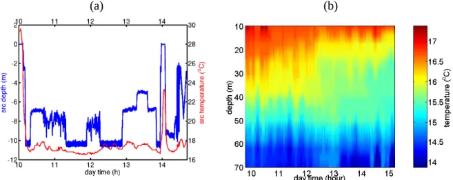
Pressure and temperature sensors were installed on the towfish to estimate source depth and temperature. Fig. 3(a) shows the source depth and temperature recorded on 24th June. Field calibration transmissions started at 10 a.m. and finished at 14 p.m. During this period, the temperature at the source is about 17.5ºC. The maximum source depth is about 10.5m and it occurs when the boat drifts. When the boat acquires speed of 2 or 4 knots source depth is around 7/8m and 5m, respectively. One can remark that in some periods, around 11 and 12 am, source depth is not stabilized, since one can notice important instantaneous vertical displacements. AOB22 has an array of 16 low resolution (0.5ºC) temperature
sensors collocated with the hydrophones. Fig. 3(b) shows the temperature data acquired by the AOB22 during 24th of June. The figure suggests that the AOB22 crossed a front in the middle of the period.
(a) (b)
Fig. 3 Temperature at the source and source depth (a) Temperature profiles acquired by the AOB22 temperature sensor array (b).
For field calibration purposes the probe signals transmitted were in the 500-2000Hz band, consisting in sequences of : ten, one second long, 500-1000Hz linear frequency modulated upsweeps 250ms apart; fifteen, half a second long, 1000-2000Hz linear frequency modulated upsweeps, 125ms apart; and fifteen second long mixture of eleven tones (multitones) covering the 500-2000Hz band. Those sequences were repeated in periods of 10-20 minutes. The signals at the hydrophones were acquired at a sampling rate of 50kHz. Since, the signals used in field calibration are bellow 2kHz, the acoustic data were downsampled to 5kHz. Figure 4 shows a spectrogram of acoustic data sample acquired on 24th June, at 12:57 pm, on hydrophone 8 of AOB22 at an approximate depth of 46m and
source-receiver range of 5km.
ACOUSTIC CHANNEL CHARACTERIZATION
The channel impulse response, which is a sequence of echoes heard at a hydrophone due to a broadband source signal, is a very robust way to characterize channel features. The signature in impulse responses of source depth, source range and their displacements, surface tides, internal tides and sediment sound speed are extensively described in the literature[2-4]. Several authors have used methods based on the estimates of the channel impulse response to estimate the source range and depth or to track internal waves[2-4]. In active tomography, where the probe signal is known and controlled, the simplest method to estimate the channel is the so called pulse compression that is the cross-correlation of a broadband signal transmitted by the source with the waveform acquired by a hydrophone. Very often in order to eliminate the lack of source phase information, and phase modelling
errors, one is interested in the arrival pattern, what is the envelop of the pulse compressed signal.
Fig 4 Field calibration waveform received at hydrophone 8 at 34m depth.
In CALCOM’10 a reference hydrophone at the source was not available, thus the signal loaded to the signal generator at the source was used for pulse compression. In order to diminish the variance of the arrival patterns presented next, those were computed by averaging the arrival pattern obtained from a single LFM within each one minute sequence. This corresponds to 15s averaging period for both type of LFM, being used 10 LFM in the 500-1000 Hz band and 15 LFM in the 1000-2000Hz band.
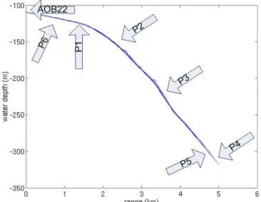
Fig. 5 Bathymetry along the slope. The arrows shows the location of the field calibration events and the receiver array
Next it is discussed the arrival patterns observed at different moments of transmission of the field calibration signals. Since the arrivals patterns obtained for both LFM are very similar, only those derived from higher frequency band LFM will be presented, because of
their broad frequency band give rise to narrower peaks. Those transmissions occurred from 500m to 5km along the bathymetry shown in Fig. 5(a).
(a) (b)
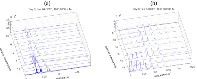
Fig. 6 Arrival patterns at hydrophone at 54m when the source is at ranges between 600m and 1.6km (a), and the sources is at ranges between 4.4 and 5.0km
Figure 6(a) presents arrival patterns at ranges between 0.6 and 1.6km, which correspond to a relative shallow water area (event P6, water depth around 120m). It can be seen that the number and time spread of arrivals increase with the distance. One can note that the number of peaks in the different arrival packets is well resolved. It is also straightforward to see that due to arrivals interference some peaks at the beginning of arrival patterns for longer distances are cancelled. As expected the number and time spread of arrival in Fig. 6(b) is higher since they were observed at a longer distance (5km). Moreover, due to the different distances, the amplitude of peaks in Fig 6(b) are 30 time weaker than those on Fig 6(a).
(a) (b)
Fig 7 presents the arrival patterns observed along the array at a distance of 600m, (a), and 4.5km, (b), from the source. In addition to the observations made for Fig. 6, this figure shows also arrival fronts impinging the array and their direction. The later arrival fronts show steepest angles, since they are related to rays that suffer several surface and bottom reflections. The number of arrivals in each arrival packet and their separation in time depends on the depth of the hydrophone. At shallow hydrophones, the surface reflected arrival fronts interferes with bottom reflected ones and two packets of two arrivals merge into a single packet of four or three arrivals. It is straightforward to see that a similar interference occurs at deeper locations, which are not sampled by array the array. Also, one can observe the cancelation of the first arrival at shallow hydrophones at range 600m.
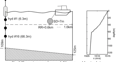
Fig. 8 The environmental setup of P6 event used for simulations
ACOUSTIC CHANNEL MODELLING
Since, the structure of the arrival pattern is very sensitive to geometrical and environmental characteristics of the propagation channel, the comparison between observed and modelled arrival patterns using available information gives some insight about the correctness of that information. Understanding the differences is fundamental to setup the parameterization and the parameters bounds for the inversion procedure.
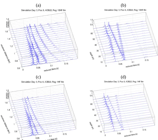
The environmental setup used for simulations, depicted in Fig. 8, is based on the conditions of event P6: source-receiver range between 0.6 and 1.6km, source depth 7m, water depth ranging from 109m at receiver location to 125m at a receiver range of 1.6km. The sound speed profile considered in simulations is the mean sound speed profile derived by the Mackenzie formula from the temperature data acquired by the temperature sensor array at the receiver, assuming a constant salinity of 36ppm for the layers covered by the array and the mean profile described in reference [5] for the deeper layers. The source range was derived from GPS information, the source depth from the pressure sensor at the source, the bathymetry from the available bathymetry map. Figure 9 presents the modelled arrival patterns under the same conditions as those of Fig. 6(a) and Fig 7(a). The arrival patterns were modelled using the Bellhop ray tracing model.
(a) (b)
(c) (d)
Fig. 9 Modelled arrival patterns at hydrophone at 54m depth, with sediment sound speed 1650m/s (a) and 1550m/s (c); and modelled arrival patterns for all hydrophones at 600m range, being the sediment sound speed 1650m/s (b) and 1550m/s(d)
There is no available detailed sea bottom data for the region, only a descriptive classification can be found [6]. The bottom is described as silty, thus it is assumed a sediment (compressional) sound speed of 1650m/s, a density of 1.7 and an attenuation of 1.0 dB/λ. The modelled arrival patterns obtained are shown in Fig 8(a) and (b), which compare favourably with Fig 6(a) and Fig 7(a), respectively. One can observe that the structure of observed and modelled arrival is similar, but the number and strength of late arrivals is greater in modelled arrival patterns than in the observed ones, which suggests that the bottom is softer than the bottom assumed in the model. Fig. 9(c) and (d) show the modelled arrival patterns where the bottom sound speed was changed to 1550m/s, and density to 1.5. The attenuation was unchanged. It is straightforward to see that the match between the modelled structure of late arrivals and observed ones resulted improved with the new value of the sediment sound speed.
(a) (c)
(b)
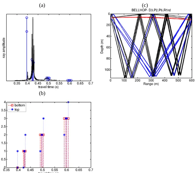
Fig. 10 Model outputs for the arrival pattern of hydrophone at 10m in Fig. 8(d): amplitudes of modeled eigenrays with superimposed acquired arrival pattern (a), number of bottom and surface bounces (b) and eigenray paths (c).
Another interesting feature observed on the arrival patterns in Fig. 7(a) is the cancellation of the first arrival in hydrophones close to the surface. In modeled arrival patterns this phenomenon thus not occurs, however the strength of the first arrival in hydrophones close to the surface is smaller than in deeper hydrophones. The model outputs relative to the arrival pattern for the hydrophone at 10m in Fig 9(d) are shown in Fig. 10: amplitude-delay of the eigenrays (a), their number of bounces (b) and paths (c). On can see, that the first peak on the arrival pattern is due to direct eigenrays and surface reflected eigenrays. Although the amplitudes of that first packet of arrivals estimated by the model are the greatest, due to their relative phases and relative instant of arrival, they sum destructively. In fact, due to the sound speed profile and/or source/receiver depth and distance this packet of arrivals can be cancelled at all, what most likely happens in arrival patterns observed in Fig. 7(a). The arrival pattern in Fig. 7(a) relative to the hydrophone at depth 10m is superimposed to eigenray amplitude-delay plot in Fig 10(a). Despite the amplitude of the
first arrival, the structure of modeled and observed arrivals is in good agreement. The amplitude of the latest packet of arrivals (centered at 0.6s) predicted by the model is small due to several (3) reflections in the bottom, thus it is embodied in the noise in the observed arrival pattern (not shown).
CONCLUSIONS AND FUTURE WORK
This paper presented a preliminary data analysis of the field calibration data set acquired during the CALCOM’10 experiment. It is described the experimental setup and the acquired data, in particular during day 24th June 2010, when the source moved in a range dependent bathymetry track along the steep slope to the deeper ocean. It was discussed the observed estimates of the channel impulse responses at different source-receiver distances and along the array depth. The data acquired shows good quality, sampling the interest area in a convenient way in order to quantify its variability by acoustic inversion. It was also discussed preliminary forward modelling as a preliminary step for the parameterization of the inverse problem. The next step in processing this data set is to systematically estimate relevant parameters to acoustically characterize the interest area. The ultimately objective is to develop a tool to be used at developing stage and to allow developers to optimize the number and location of wave energy generators and predict their influence in underwater noise in surrounding areas.
ACKNOLEDGMENTS
This work was partially supported by project WEAM (PTDC/ENR/70452/2006), funded by FCT, Portugal and the ESONET NoE (contract #036851) funded by the the UE.
REFERENCES
[1]M.B. PORTER, The BELLHOP Manual and User’s Guide: PRELIMINARY DRAFT,
Heat, Light, and Sound Research, Inc. technical report, La Jolla, CA, USA,May, 2010.
[2]M.B. PORTER, S.M. JESUS, Y. STEPHAN, X. DEMOULIN and E.COELHO, Tidal effects on source inversion, Experimental Acoustics Inversion Methods for Exploration
of the Shallow Water Environment , Ed.Caiti, Hermand, Jesus and Porter,
KLUWER,1999.
[3]S.M. JESUS, M.B. PORTER, Y. STEPHAN, E.F. COELHO and DEMOULIN X, Broadband localization with a single hydrophone, Proc. MTS/IEEE OCEANS'98, Nice, France,1998.
[4]P. FELISBERTO, S.M. JESUS, Y. STEPHAN and X. DEMOULIN, Shallow water tomography with a sparse array during the INTIMATE'98 sea trial, Proc. MTS/IEEE
[5]S. SALON, A. CRISE, P. PICCO, E. MARINIS and O. GASPARINI, Sound speed in the Mediterranean Sea: an analysis from a climatological data set, Annales Geophysicae, European Geosciences Union, 21:833-846, 2003.
[6]F.C. LOPES, P.P. CUNHA, A plataforma continental algarvia e províncias adjacentes: uma análise geomorflógica, Ciências Geológicas-Ensino e Investigação e sua História, 2010.