Machine learning in analytical chemistry: applying innovative data analysis methods using chromatographic techniques

Diogo Barros Gonçalves

Diogo Barros Gonçalves

Machine Learning in Anal

ytical Chemis tr y : appl ying inno vative dat a anal ysis me

thods using chromatographic techniques

Machine Learning in Analytical Chemistry: applying innovative data analysis methods using chromatographic techniques

University of Minho

Diogo Barros Gonçalves

Machine Learning in Analytical Chemistry: applying innovative data analysis methods using chromatographic techniques

Msc. in Chemical Analysis and Characterisation Techniques

Chemical Sciences

Supervisors:

Professor Pier Parpot

Professor Nuno Castro

University of Minho

School of Sciences

Agradecimentos

Deixo aqui expresso o meu agradecimento a um alargado leque de pessoas cujo contributo para este trabalho foi, de diversas formas, relevante.

Aos meus orientadores, Pier Parpot e Nuno Castro, pela oportunidade dada de trabalhar nesta interface, pelo apoio durante a realização deste trabalho e por me terem conferido a autonomia para explorar o tema da maneira que me pareceu mais adequada.

Gostaria de agradecer também à Fundação para a Ciência e Tecnologia através do projeto POCI-01-0145-FEDER-029147 - PTDC/FIS-PAR/29147/2017 financiado por: OE/FCT, Lisboa 2020, Compete 2020 POCI, Portugal 2020 FEDER.

Ao pessoal do LIP e do laboratório 56 pela camaradagem, em especial ao Tiago Vale pelo apoio e entusiasmo partilhado no desenvolvimento do trabalho.

Ao Rafael pelo companheirismo ao longo do nosso percurso académico, em especial pela

partilha de entusiasmo pelas aplicações e potencial de machine learning bem como pelo suporte

incondicional. À Luz, por tudo, mas especificamente pelo apoio e paciência no processo de escrita. ^^ Parecia-me algo egoísta não expressar uma palavra de apreço aos colaboradores da NVending que, ao longo do ano, foram garantindo que havia café nas máquinas.

Last but not least, à minha família e a todos os meus amigos. Em especial aos meus irmãos, aos meus pais, e à minha avó.

Resumo

O constante avanço científico-tecnológico permitiu que, ao longo do último século, as técnicas de análise química extraíssem cada vez mais conhecimento das amostras analisadas. Nos últimos anos, a quantidade de dados que as mais recentes técnicas analíticas produzem possui uma dimensão tão elevada que a sua análise é denominada de análise megavariacional. Recentemente, a aplicação de

ferramentas de machine learning em análises de dados químicos tem permitido extrair informação

relevante das amostras analisadas que até recentemente não era possível.

Com isto em mente, o objetivo deste trabalho consiste em classificar condições de manufatura de placas de circuito impresso tendo por base dados provenientes de análise por cromatografia líquida acoplada a espetrometria de massa com extração sólido-líquido. Desta forma, esta dissertação está dividida em duas partes: a primeira sintetiza o trabalho efetuado para garantir que o método de análise produz dados com qualidade adequada para que na segunda parte esses dados sejam usados para construir modelos preditivos. Paralelamente, foi desenvolvida uma técnica de aumento de dados que, até onde o nosso conhecimento vai, constitui a primeira técnica de aumento de dados desenvolvida para problemas de classificação com dados provenientes de análises cromatográficas.

Os resultados dos melhores modelos mostram precisões superiores a 94% para a previsão de todas as condições de manufatura. Adicionalmente, a técnica de aumento de dados desenvolvida mostra desempenhos superiores comparativamente a outras técnicas de aumento de dados.

Em síntese, os resultados obtidos indicam que, para além de distinguir classes com composições químicas diferentes, é possível adquirir informação sobre quais são os compostos químicos que distinguem as classes em estudo. Esta informação pode vir a ter uma importância significativa em áreas como controlo de qualidade, química alimentar e indústria fito-farmacêutica.

Abstract

Scientific and technological advances allowed the extraction of a growing quantity of knowledge from the analysed samples by means of analytical techniques. Over the last few years, the dimensionality of data that the most recent analytical techniques produce is so high, that its analysis is now called megavariate analysis. Recently, the usage of machine learning tools in chemical data analysis have allowed the extraction of relevant information from samples at a level which, until then, would just not be possible.

The objective of this work consists in classifying manufacturing conditions of printed circuit boards based on data acquired by SLE-HPLC-ESI-MS. As such, this dissertation is divided in two parts: the first synthesizes the work taken to assure the analytical method produces data with adequate quality in such a way the second part shows the development of predictive model using the previous acquired data. At the same time, a data augmentation technique which, to the best of our knowledge, constitutes the first time a data augmentation technique for classification problems using chromatographic data, has been developed.

Best models’ results show precisions above 94% for all manufacturing conditions prediction. Moreover, the developed data augmentation technique reports superior performances when compared to three other data augmentation techniques.

In summary, the results show that, besides distinguishing classes with different chemical compositions, it is possible to obtain information about which are the chemical compounds that differentiate the classes. This information might be of significant importance for areas such as quality control, food chemistry, botany and pharmaceutical industry.

Contents

Agradecimentos ... iii

Resumo ... iv

Abstract ... v

Contents ... vi

List of abbreviations, acronyms and symbols ... viii

Chapter 1 – Introduction ... 1

1.1. Motivation for this Master Thesis ... 1

1.2. Document structure ... 2

Chapter 2 – Background ... 4

2.1. From problem definition to data interpretation: stages of the Analytical Chemistry Process ... 4

2.1.1. Problem Definition and Method Selection ... 4

2.1.2. Sampling ... 5

2.1.3. Sample Pre-treatment ... 6

2.1.4. Chemical Analysis ... 8

2.1.5. Data Interpretation ... 10

2.2. Towards the fully exploitation of Chemical Data ... 12

2.2.1. Brief overview on the history of Machine Learning ... 13

2.2.2. Learning paradigms in Machine Learning ... 14

2.2.3. Machine Learning Workflow ... 16

2.2.4. Introduction to Learning Algorithms ... 19

2.3. Bridging Analytical Chemistry and Machine Learning ... 27

2.3.1. Motivation and applications of Machine Learning in Analytical Chemistry ... 28

Chapter 3 – Experimental ... 30

3.3. Reagents ... 32

3.4. Preparation of solutions ... 32

3.5. Sample Preparation ... 32

3.6. Instrumentation ... 33

3.7. Software and hardware ... 33

3.8. Data mining methodologies ... 34

Chapter 4 – Results and Discussion ... 35

4.1. Overview ... 35

4.2. Optimization of the analytical method ... 36

4.2.1. Chemical Analysis – HPLC-MS ... 36

4.3. Machine Learning Model Development ... 38

4.3.1. Exploratory Data Analysis ... 39

4.3.2. Time approach ... 43

4.3.3. Mass approach ... 47

4.4. Structure elucidation from feature importance using ESI-MS/MS ... 52

4.5. Data augmentation technique ... 53

Chapter 5 – Conclusions and future work ... 59

List of abbreviations, acronyms and symbols

AAS Atomic absorption spectroscopy

ADASYN Adaptative synthetic sampling

AES Atomic emission spectroscopy

AI Artificial intelligence Avg Average CE Capillary electrophoresis DA Synthetic data DLS USD

Dynamic light scattering United States dollar

DNN Deep neural network

DoE Design of experimental

DSC Differential scanning calorimetry

DT Decision tree

ESI Electrospray ionisation

FIA Flow injection analysis

FTIR Fourier-transform infrared spectroscopy

GBM Gradient boosting machines

GC Gas chromatography

GOFAI Good old-fashioned AI

GSR Gunshot residue

HPLC High performance liquid chromatography

HSSE Headspace solid extraction

IC Ion chromatography

IPA Isopropyl alcohol

IPC Association connecting electronic industries

LLE Liquid-liquid extraction

LR Logistic regression

Max Maximum

MC Manufacturing condition

ML Machine learning

MS Mass spectrometry

MVA Multivariate analysis

NASA National Aeronautics and Space Administration

NMR Nuclear magnetic resonance

OD Original data

PC Principal component

PCA Principal component analysis

PCB Printed circuit board

PTFE Polytetrafluoroethylene

QPPR Quantitative pattern-pattern relationship

Q-ToF Quadrupole time-of-flight

QqQ Triple quadrupole

QSAR Quantitative structure-activity relationship

QSRR Quantitative structure-retention relationship

RF Random forest

ROS Random over-sampling

SBSE Stir bar sorptive extraction

SLE Solid-liquid extraction

SMOTE Synthetic minority over-sampling technique

SPE Solid-phase extraction

SPME Solid-phase microextraction

SS Standard scaler

SVM Support vector machines

t-SNE t-distributed stochastic neighbour embedding

TGA Thermal gravimetric analysis

TIC Total ion current

UHPLC Ultra high performance liquid chromatography

UV-Vis Ultraviolet-visible

XGB Extreme gradient boosting

Chapter 1 – Introduction

1.1. Motivation for this Master Thesis

Analytical chemistry is one of the several chemistry fields with deep implications across almost all branches of science and even more importantly, our society. As such, the working methodology is

well-defined where five main steps can be identified as defined by Elving back in 19501.

Every work starts with the problem definition and method selection. It is supposed to define the motivation of the work, how it will be tackled and by what means. Typically, a vast search across reliable sources - such as peer-reviewed journals and specialty bibliography - comprises its core.

After a proper definition on how the challenge will be tackled, the next two steps concern the sampling process and sample pre-treatment. They are considered crucial to the analytical process since the results obtained from chemical analyses will be as good as the sampling and sample pre-treatment performance. These steps are often tedious and time-consuming requiring high consistency across all samples and days which makes automation a tempting solution massively applied both by industry and academia.

The next stage is the core of the analytical process in which the data necessary to answer the previously stated question is acquired. With the evolution of analytical techniques and equipment, the labour part traditionally done by analytical chemists is being rapidly and steadily replaced by automation.

The last step of the analytical process - data interpretation - is the key point of the analytical process. It is often performed by a skilled operator where a series of complex approaches are executed to achieve the so wanted answer to the stated question. In contrast with the other stages, data Interpretation is falling behind in terms of automation since it requires an intuitive intelligent approach

compared to the easy programmable tasks which is somehow related with both sampling/sample

successfully applied in several science fields, allowing both automation and - even more importantly - the discovery of underlying patterns in data that could hardly be found by other means.

In this context, the aim of this master’s thesis consists in combining machine learning methods with chemical analyses focusing in two points:

- Development of models which are able to classify samples according to different relevant parameters (i.e., manufacturing conditions).

- Exploitation of model decision in order to extract new knowledge from sample nature.

1.2. Document structure

The developed work presented in this dissertation focused in the application of machine learning in analytical chemistry. More precisely, the development of machine learning models to classify samples according to chemical data. The first part of the project consists of generating chemical data by selecting, extracting and analysing samples whilst the second relates to all the data mining work carried on to extract knowledge out of the chemical data.

The project work is presented in five chapters. The first serves as guide for orientation purposes to the whole the document.

The aim of Chapter 2 is to bridge analytical chemistry and machine leaning by approaching both analytical chemists to machine learning as well as machine learning researchers to analytical chemistry. This way, the first part focus on a chronological introduction of the methodology carried on by analytical chemists whereas the second aims to introduce basic notions of machine learning for analytical chemists. Chapter 2 is concluded with a brief overview of recent works on the interface between these two areas with a special focus on chromatography techniques.

Chapter 3 presents the technical descriptions of the developed work, both regarding analytical chemistry and data mining.

Chapter 4 reports the discussion of results obtained during work development while Chapter 5 includes the major conclusions drawn as well as suggestions for future work regarding this interface between machine learning and analytical chemistry.

Chapter 2 – Background

2.1. From problem definition to data interpretation: stages of the Analytical Chemistry

Process

Analytical chemistry can be defined as the study of substances in a matter of separation,

identification and quantification2. It has a crucial role across different areas such as environment3–7 (e.g.

analysis of environmental microplastics), medicine8–14 (e.g. clinical diagnosis), agriculture15–21 (e.g.

pesticide analysis) and even some more broad areas such as biology22–26 (e.g. microbiological analysis of

food) and geology27–32 (e.g. mineral inorganic content). Even though these application areas developed

internal analytical processes aiming to increase their work performance according to domain specificities, a common work pipeline can be identified where five main steps are stated: problem definition and

method selection, sampling, sample pre-treatment, chemical analysis and data interpretation1. Along this

section, the first four subsections will be briefly discussed with a special focus on data interpretation.

2.1.1. Problem Definition and Method Selection

Intuitively, every work starts with the definition of what question will be subject of study. The goal of this initial stage is to translate broad, domain-free, general questions into well-defined, specific questions whose answers can be achieved using chemical measurements (i.e. “how can printed circuit boards’ (PCBs) manufacturing conditions be related with its chemical composition?” should be translated to something like “how can PCBs’ chemical composition be analysed?”). What type of sample has to be collected/analysed? What kind of sample preparation has to be performed? Which analytical techniques/setups are most suitable for this end?

After proper definition, the operator is taken into domain-specific questions regarding the method selection. What is the budget and time available to achieve desired results? How will samples be collected? Which sample preparation technique should be applied in order to fulfil the pre-stated needs?

What performance requirements threshold should be guaranteed for the analysis (specificity, selectivity, accuracy, precision, etc.)? How will the acquired data address the ultimate question (keep this one in mind!)?

For this end, the operator usually combines experience with published works in peer-reviewed journals and specific bibliography since all of these questions must be well-stated before diving deep into the lab work.

2.1.2. Sampling

‘Sample’ can be defined in several different ways according to the work stage the analyst is

referring to, which led to define ‘sample’ according to the stage the analyst is mentioning33. Due to its

ubiquitous mentions across all stages - when considering sampling - a more specific sample definition

can be used as “a portion of material selected from a larger quantity of material”33,34.

The objective of sampling consists in obtaining a small, representative and homogenous sample.

A schematic sampling process is depicted in Figure 135.

The sampling process starts with getting a bulk sample from a lot. A lot represents the total amount of material you have access to regarding your study object (e.g. several PCBs manufactured under different conditions). A bulk sample is still a large sample that it is taken from a lot (e.g. get an adequate number of PCBs produce under the same conditions). This bulk sample must be representative of the lot, i.e.,

Lot

Bulk

sample

Laboratory

sample

Aliquot

must gather chemical properties which illustrate the typical behaviour observed in the lot. The laboratory sample is obtained after the bulk sample has been properly prepared (e.g. cut PCBs in halves and shuffle samples produced under the same manufacturing conditions). The extension/number of stages the

sample is exposed during sampling must be kept minimal in order to minimize the sampling error36.

Then, the aliquot is achieved once a small portion is taken from the bulk sample and ready to be submitted to sample pre-treatment.

2.1.3. Sample Pre-treatment

In case the sample is not in a suitable shape to be analysed directly, a middle step between sampling and chemical analysis has to be performed. This stage can have multiple purposes like clean-up, concentration, interference elimination, speciation or extraction. The extension of this stage is mostly dependent on the sample nature, matrix, concentration level of the chemical compounds which are going

to be evaluated during the analysis and the employed analytical technique37. This information can be

summarized as in Table 1 where it shows that the pre-treatments a sample is submitted to can be related to the analyte nature.

Analyte Sample pre-treatment

Organics Extraction, concentration, clean-up, derivatization

Volatile organics Transfer to vapor phase, concentration

Metals Extraction, concentration, speciation

Metals Extraction, concentration, speciation

Ions Extraction, concentration, derivatization

Amino acids, fats carbohydrates Extraction, clean-up

Microstructures Etching, reactive ion techniques, etc.

Since it is not a matter of subject for this dissertation to discuss each of them, a brief overview of sample pre-treatment concerning organic/organic volatiles will be carried on with a special focus on solid-liquid extraction (SLE).

There are four widely used techniques for extraction of organic/organic volatile compounds: solid/liquid-liquid extraction (SLE/LLE), solid-phase extraction (SPE), solid-phase microextraction (SPME) and stir bar sorptive extraction (SBSE). Every extraction technique takes advantage of chemical properties which are used to influence the distribution of the analyte between phases. These properties include hydrophobicity, solubility, vapor pressure, molecular weight and dissociation constants of acids and bases. To understand how an extraction can be optimized one must be aware of the chemical equilibrium which is undergoing in the system as

X

⇌ X

and equilibrium constant,

K

=

[X]

[X]

where equation 1 denotes the chemical equilibrium between phase A and phase B at a given

temperature and equation 2 represents the equilibrium constant, KD, where [X] represents the

concentration of X at a given temperature. The extraction conditions must be defined in order to increase the analyte concentration in phase B, i. e., to maximize the equilibrium constant.

In SLE, the objective is to extract as much analyte as possible from phase A (solid) to phase B

(liquid) using a limited amount of solvent aiming to obtain an extract as concentrated as possible38. In

most cases a single-stage extraction is not enough to fulfil the desired specifications and a multi-stage extraction is required. They differ in the number of times phase A is submitted to fresh solvent (phase B). Different modifications can be applied in order to steer different chemical properties such as solubility

(HSSE) are preferred, recent developments in SLE techniques show great efficiency improvements and

greener alternatives when compared with state-of-the-art techniques42.

Apart from the employed methodologies, by the end of the pre-treatment, samples must be in a suitable form to maximize the efficiency of the essential step of the analytical chemistry process: the chemical analysis.

2.1.4. Chemical Analysis

“Chemical analysis began on the 8th day. Adam, recovering after cooperating with god, in creating Eve, felt first pangs of hunger. He went around and harvested different kinds of colorful berries [eyes as

detector] and set down for dinner with Eve. Eve rejected some berries due to foul smell (nose as detector).

The bitter tasting ones were rejected next (taste as detector), and the delicious ones were consumed. Thus, first chemical detectors were nose, tongue, and eye; the five senses were used as chemical detectors for a long time.”43

Albeit not even close to the objective truth science looks after, this excerpt exceptionally captures the inquisitive nature of human beings and how it is used to understand the world. In fact, humanity has been using their five senses as detectors for a long time. However, it was not until Dutch scientists discovered how to attach two lenses in line with one another to improve their visual ability that modern

analytical science came to be44,45.

Chemical analysis consists in the determination of the chemical composition of substances. “In

other words, it is the art and science of determining what matter is it and how much of it exists”46. It can

be divided in two branches: qualitative and quantitative chemical analysis. Qualitative chemical analysis studies what matter is it, whilst quantitative chemical analysis is responsible for answering how much of it there is. Additionally, when considering the employed technology two more subdivisions come along:

classical, wet chemical methods and modern, instrumental methods47. These differ mainly on the used

technology and subsequently the magnitude of results one can accomplish48. Most classical analytical

methods rely on chemical reactions to obtain results (e.g. acid-base titration) whereas modern analytical methods typically measure a certain physical property of the analyte (e.g. UV—Vis spectrophotometry). Obviously, modern methods yield better results (higher sensitivity, specificity, precision, accuracy, low

time, ease-of-use, etc.) but they also carry some drawbacks (high cost, higher uncertainties, black box

syndrome,etc.) when compared to classical methods49,50.

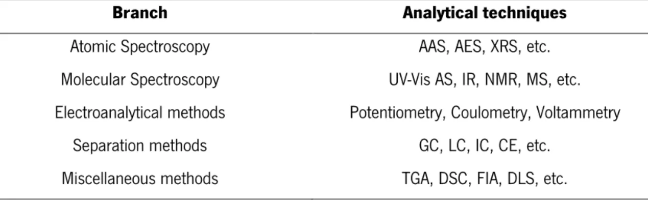
Modern methods comprise a broad range of different methodologies to quantitively address the pre-stated question. The vast different analytical techniques can be subdivided according to the measured

physical property which in turn can be divided in five different families as shown in Table 22. It

summarizes a wide range of different analytical techniques usually applied in this stage.

Table 2 - Different analytical techniques subdivided by chemistry branches

Branch Analytical techniques

Atomic Spectroscopy AAS, AES, XRS, etc.

Molecular Spectroscopy UV-Vis AS, IR, NMR, MS, etc.

Electroanalytical methods Potentiometry, Coulometry, Voltammetry

Separation methods GC, LC, IC, CE, etc.

Miscellaneous methods TGA, DSC, FIA, DLS, etc.

These techniques are often combined in order to maximize the chemical information the analyst can get. From all of them, separation methods are one of the most developed branches. Back in 2013,

its value market was $7 billion USD with a prospection for 2018 of $10 billion USD51. Within this industry,

liquid chromatography (LC) represents the large segment due to its massive use in areas such as

Chromatography came a long way since 1903 when a Russian botanist named Mikhail Tsvet

discussed his recent research on leaf pigments and a novel way to separate them53,54. Although it was

generally well accepted by the community (with even some scientists referring the crucial role Tsevt’s

research had in the work of Nobel Prize laureates from that epoch55) it was not until the Second World

War, the Manhattan Project and the urge to find a way to purify rare-earth metals that chromatography

gained its momentum, starting with ion chromatography56. Gas-liquid chromatography (GC) was

developed faster than high pressure liquid chromatography (HPLC) where the first paper by James and

Martin on GLC was published in 195257. Fifteen years later the first paper describing an HPLC apparatus

was published giving rise to the massive chromatography market we have today58. Nowadays, HPLC and

Ultra HPLC (UHPLC) coupled with mass spectrometry detectors (MS) have been widely applied in a huge

array of works ranging from clinical to beverage industry59–64. The evolution of MS gave rise to a panoply

of mass analysers where quadrupole time-of-flight (Q-ToF) and triple quadrupole (QqQ) are currently

considered top choices regarding both quantification and structure identification, respectively65,66. The

combination of MS with more conventional detectors such as fluorescence or diode array exponentially increased the amount of data the analytical chemist can now acquire regarding its experiments which in turn increased the need to improve his/her arsenal of data interpretation tools in order to tackle these challenges.

2.1.5. Data Interpretation

The last step of the analytical chemistry process consists in understanding what the acquired chemical data allows to conclude about the problem definition. This need led to the employment of statistical tools to study how chemical data relates with the pre-defined question. The first paper describing the use of multivariate regression methods and design of experiment (DoE), in analytical

high-dimensionality associated with areas as spectrophotometric analysis or proteomic, multivariate analysis

(MVA) started to be applied in the sixties68–71. In its core, MVA consists in simultaneously analysing many

variables in order to understand how these variables correlate with each other72. Table 3 shows how

data dimensionality relates with the statistical type.

Table 3 - Relationship between dimensionality and statistics type.

Dimension Sample set Statistics

1-D Vector Univariate

2-D Matrix Bivariate

n-D* n-D array Multivariate

* n ≥ 3

MVA allowed interesting breakthroughs back then due to its ability to analyse high dimensionality data (a difficult task for humans when n > 3) and to allow the analytical chemist to get insights from that. Although great achievements were performed with MVA’s application in data interpretation, its application were mostly based on multivariate regression methods, response surface’s and pattern recognition. With the ever-increasing amount of data acquired with novel technology and the rise of artificial intelligence (AI) and machine learning (ML) methods powered by works as Samuel’s AI system which was capable to learn how to play checkers, it was a matter of time until ML methods started to be

employed in analytical chemistry73,74. Samuel also defined ML as “the field of study that gives computers

the ability to learn without being explicitly programmed”73. In fact, an important catalyst in bridging ML

and chemistry were NASA’s moon missions and their need for organic chemists to develop AI systems

for structure elucidation70,75. By the eighties, chemometrics took off as a research field of analytical

chemistry with its early applications in high-dimensionality areas such as LC and spectrophotometry76–81.

allowed a better understanding of high-dimensional chemical data but also generated good practices in the sampling step with the common use of DoE.

In the beginning of this decade, a series of fortunate events led to another revolution concerning

data interpretation: the rapid growth of the technology around graphics processing units83,84, powerful

cloud-computing systems85 and a society where more data is generated in one year than in the entire

history of mankind86 substantially contributed to major breakthroughs in AI and ML. In turn, the

widespread application of these tools led to the development of easy-to-use, open-source software87 and

a strong community which allowed researchers from fields other than computer science to embrace ML in their works. Analytical chemistry is no exception and the application of these novel tools permitted that the insights hidden in chemical data (often called megavariate data) acquired by several different methods could be strongly scrutinized. In what concerns the analytical chemistry process, this came to be its last big update in a long time.

2.2. Towards the fully exploitation of Chemical Data

After exploring the Analytical Chemistry Process step by step, it became clear how can one benefit from the application of ML tools in the process itself. Along this second section of the chapter, a special focus will be given to the introduction of non-technical, relevant topics of ML for analytical chemists with little to null experience in this area.

The first subsection gives a brief overview on the history of ML from Dartmouth to present days, following the presentation of the most important steps regarding ML workflow, ending with the introduction of the intuition behind ML algorithms which were used in the development of this dissertation.

2.2.1. Brief overview on the history of Machine Learning

The history of ML is deeply connected with AI. One possible definition of intelligence would be

“the ability to achieve complex goals”, therefore, AI could be defined as “non-human intelligence”88.

It is generally accepted that the term “artificial intelligence” was officially coined in Dartmouth in

1956 by a group of scientists whose question was: “can a machine be capable of thinking?”89. To do so,

first approaches involved having programmers using their skills to handcraft a series of long and explicit

rules. This is known as symbolic AI and it was the dominant paradigm of AI during many years90. Of

course, symbolic AI (or good old-fashioned AI, GOFAI) proved to be an adequate approach in logical,

well-defined problems whose ruling principles are known and, for that reason, easy to instruct a machine to

do (e.g. having a GOFAI beat the world chess champion91). However, when considering more complex

and intractable problems like image recognition, speech recognition or language translation, GOFAI turned not to be a suitable approach. As a result, a new approach arose in order to surpass these obstacles. Instead of having brilliant programmers instructing a machine, they would give the machine a significant amount of data and its labels (e.g. photos of cats and dogs and its proper labels) and let the machine figure out all of those rules by itself. This approach came to be known as machine learning and has ultimately revolutionize our society.

Nowadays, humanity relies on ML for a panoply of human-level tasks in domains such as communication, healthcare, energy, finance, transportation or manufacturing, to name a few. In fact, ML is so pervasive that we are constantly being exposed to its outputs and (most of the time) not even aware of it. Such controversies gave rise to voices from both sides: some envision a world where AI has a detrimental yet well-oriented role in our society whereas others fear its consequences. A recent example of the latter is whether the ultimate goal of Neuralink of merging humans and AI by developing

Although these questions are, at least, decades away, the need to regulate how these systems will work should be faced in the near future in order to be primed by the time it comes.

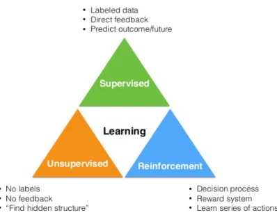
2.2.2. Learning paradigms in Machine Learning

Most authors define three paradigms concerning the process of having a machine learning which

are schematically depicted in Figure 293.

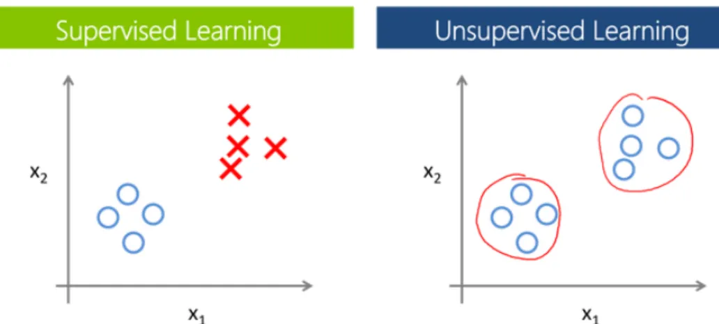
Supervised and unsupervised learning mainly differ in whether labels are given to the algorithm or not. Supervised learning’s tasks come down to classification (e.g. predict if a given sample is forgery/contaminated – discrete output) and regression (e.g. predict the concentration of a solution

based on an analytical technique signal’s response – continuous output)94. In unsupervised learning

common tasks involve clustering (e.g. group samples according to chemical composition’s similarity) or

dimensionality reduction (e.g. using less descriptors to explain how data relates)94. Figure 395 illustrates

how learning algorithms (also called learners) from these two paradigms perform.

Figure 2 - The three learning paradigms: supervised,

While supervised learners output a prediction, unsupervised learners aggregate samples according to a pre-specified metric. In chemometrics, the latter have been used for a long time to find hidden structures

related to chemical data96. Currently, unsupervised learning is widely used in exploratory data analysis

precisely due to its ability to aggregate samples into clusters that are somehow chemically related, which

in turn allows the analyst to understand unknown patterns regarding the analysed samples97. Other

applications consist in data dimensionality reduction which decreases the number of descriptors needed

to describe how samples relate with its variables98. Synergies between these two paradigms integrate the

typical ML workflow in several fields, including analytical chemistry.

Despite these differences, the aforementioned paradigms have a specificity in common: the output they produce is based on their input data, i. e., they both learn from previous knowledge. This constraint is not applied in reinforcement learning where the agent learns by experience as shown in Figure 4.

Figure 3 – Main differences between supervised and unsupervised learning. (adapted from ref 95)

action reward

Agent

Although reinforcement learning is mostly applied in robotics99,100, text mining101,102and

healthcare103,104, several science fields have embraced its application and conducted interesting studies.

In organic chemistry, a recent study showed that it is possible to optimize the experimental conditions

of chemical reactions by applying this methodology105.

2.2.3. Machine Learning Workflow

To understand how ML can be a valuable resource in analytical chemistry, it is important to comprehend the basics behind a ML workflow. To do so, this subsection introduces important steps that comprise a supervised learning workflow where Figure 5 shows a simplistic schematic representation of it. Some steps (e.g. data preparation, data splitting, feature engineering, hyperparameter optimization evaluation, etc.) which would require further explanations were removed for interpretation purposes.

x x

Data ML Predictions

(a) – From data to predictions.

(b) – Evaluating predictions. Data ML Predictions Evaluation Data ML Predictions Evaluation Model selection

Data Hyperparameter _optimization Predictions

Evaluation

Model selection

x

Production

data

Best model

Predictions

(e) – Model ready to real world application.

(a) to (b)

(b) to (c)

(c) to (d) (d) to (e)

ML model development simplistically consists in feeding the learner an adequate amount of data so it can learn the function which maps how data relates and, ultimately, provide as output an accurate

prediction – 5(a). The accuracy of the predictions must also be evaluated – 5(b). To do so, it is

important to use a metric which concisely evaluates the model. Classification tasks typically use confusion matrixes, precision-recall, accuracy and area under the curve metrics whilst root mean square

error and root mean absolute error are preferred for regression tasks106–108_{. Once a metric is applied model}

performance can be assessed.

The next step is to apply the same methodology to several algorithms – some of them will be

introduced in the next subsection – and measure each performance – 5(c). It is important to test

different algorithms since distinctive learners will perform better depending on the input data it receives

(no free lunch theorem)109_.

Every algorithm has parameters which cannot be learnt by itself and therefore must be defined before training (the process in which the algorithm is learning the mapping function, i. e., where it figures out the rules needed to explain how data is related). These are called hyperparameters and fine tuning

them allows the algorithm to more easily capture data patterns, thus, increasing its performance – 5(d)94_.

Once the best model (function which best describes how the label is related to its input variables) is obtained and properly evaluated the model is ready to be applied with new data.

Despite the simplistic representation, Figure 5 allows a quick overview on how most ML models are built.

Another way to increase model performance consists in feeding the learner with more high-quality data. By having more data to train on, the applied learner will be able to capture complex data trends. This can be done by acquiring more data however, sometimes, this is not possible. In these cases, the analyst must resort to synthetic ways to expand the size of his(er) dataset, often called data augmentation techniques. Under an analytical chemist perspective this must be perceived as a means

of increasing the number of events (analysed samples) without further experiments (chemical analysis). Its application in ML research, is responsible for interesting achievements such as top performances in ML competitions. In computer vision (e.g. classifying pictures of dogs and cats) it can be done by applying rotations of the original pictures, changing colours, mirror effects, etc. By doing this, the analyst is feeding the learner with more data so it can find the best model. In chemistry, data augmentation techniques

are now applied by adding drifts to the original data110,111_{. This approach has been successfully applied}

with NIR and molecular descriptors using public datasets.

2.2.4. Introduction to Learning Algorithms

The last subsection introduced how a supervised ML model can be built. This subsection will introduce the intuition behind the ML algorithms which were used during the elaboration of this dissertation. The intention here is not to present the reader with all the algorithm’s mathematical formalism but rather to give an intuition on how they perform the task. If interested in the mathematics

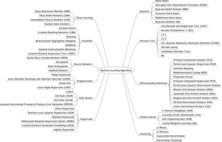
To properly introduce ML algorithms, it is important to acknowledge what it is first. In practice, an algorithm is a step-by-step way to solve a problem. As previously stated, ML algorithms are usually called learners. In contrast with common algorithms where a list of rules to follow is instructed to a machine, the conception of learners allow them to infer those rules by analysing a considerable amount of data. The plethora of academic and corporate research gave rise to a large variety of learners as stated in Figure 6113_.

This large representation intends to group learners according to operational similarity. Different families will typically perform better with distinctive datasets hence the popular no free lunch theorem applied in this domain. From this large number of learners, six of them will be covered here, particularly: principal component analysis, logistic regression, decision tree, random forest, gradient boosting machine and support vector machines.

Principal Component Analysis

Principal component analysis (PCA) is an unsupervised learner whose goals involve reducing data’s dimensionality and cluster samples according to its similarity. Widely considered the building block of chemometrics, PCA is commonly found in most chemical data analysis mainly due to its ease of

interpretability which can be stated in Figure 7114,115.

This methodology consists in the application of algebraic operations which enable dataset’s rotation in such a way that the rotated features are statistically uncorrelated. Another definition says “PCA

simplifies the complexity in high-dimensionality data while retaining trends and patterns”116_.

Applications in analytical chemistry usually tend to plot the first and second/third component in

order to explore how samples and features correlate with one another117. PCA’s main limitation concerns

the fact that the applied rotations are linear transformations of the original data. When looking for more complex data patterns, different algorithms capable of non-linear projections should be taken into account (e.g. t-SNE)118_.

Logistic Regression

The first supervised learner to be introduced is logistic regression (LR). Its conception goes back

upgrade of it. Multiple linear regression can be expressed as in equation 3 where y denotes the

dependent variable (e.g. concentration of Na+ in a solution), b are the coefficients and X are the

dependent variables (e.g. intensity of a measured signal).

y = β

_{+ β}

Χ

_{+ … + β}

Χ

Linear regression enabled analytical chemists to calculate different properties for a long time. However, linear regression has two main limitations: it assumes the relationship between y and X is linear and it outputs a continuous value from -¥ to +¥. This second limitation becomes particularly important if instead of y being a continuous variable (like in the aforementioned problem), y is a categorical value (e.g. given a series of relevant parameters, will a reaction occur or not). This is the kind of problem where

LR becomes a valuable tool. As can be seen in Figure 8120 and explained by equation 4, LR has the

advantage of outputting a value between two pre-stated values.

y =

1

1+ e

(eq. 4)

This small improvement allowed its wide use in biological sciences back in the early twentieth century

and its later application in social sciences119_{. Despite its simplicity, a recent review showed that the}

application of more complex learners over LR had no performance benefit concerning clinical prediction

models121. Nevertheless, nature provides endless situations where the problem demands more flexible

learners capable of better generalization. The next four learners will address this.

Decision Tree

A decision tree (DT) is no more than a disjunction of conjunctions. In fact, humanity applies DTs in a panoply of different problems. In order to classify rocks, high school students are given a series of rules they have to follow to reach an accurate classification. The intention is to, with each rule the student follows, increase the subset purity, i. e., decrease the number of rock possibilities’, until he reaches a

subset where only one rock class can fulfil all those specifications – Figure 9122_.

Figure 9 – Schematic representation of a decision tree criteria rules for rock classification task.

To do so, the student follows a set of rules concerning important features regarding the rock. Some features include its color, particle size, visible crystals, reactivity with certain substances, smell and even its taste. Different features will have distinct importance concerning rock classification. What high school teachers do, is to use their knowledge about geology to write that set of rules. In practice, what a DT learner does is to figure out all of those rules according to the input data it is given.

This same methodology is extensively applied in different areas including analytical chemistry.

DT’s applications not only involve classification tasks like predicting different types of wines123 but also

regression problems like predicting the relationship between structure-activity (QSAR) for a compound124.

One of the main advantages behind DT comes from the fact that the set of rules it infers enables the analyst to acquire more knowledge about the sample nature. Albeit it looks a normal requirement, state-of-the-art algorithms like deep neural networks (DNN) don’t allow such easy intuitions hence DTs widespread use in more simplistic problems.

Random Forest and Gradient Boosting Machines

One of DT’s main limitations is its ability to generalize extremely well on the training data. It typically happens when the depth of the tree and/or the number of applied splits is too large which leads to one of the trickiest obstacles in ML called overfitting. Overfitting happens when the learner exceptionally

While the black line sets an adequate decision boundary, the green line shows what happens when a model over-generalizes during its training. In real world applications, the green line model will tend to perform worse than the black line one. In a certain way, the model is suffering from “hallucinations” since it is capturing trends that don’t really exist which can be attributed to a panoply of sources of error such as noise, mislabelling, detector’s malfunctioning, among others.

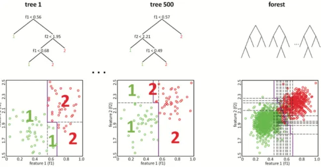
In 2001, Breiman126_{introduced the concept of random forest (RF) which, as the name implies,}

consists of a large number of DTs that operate as an ensemble – Figure 11127_.

Figure 11 - Random forests are composed by individual decision trees that act together as an

ensemble. (adapted from ref 127)

RFs tend to reduce model overfitting. By using a large number of uncorrelated trees operating as a committee, RFs are capable of outperforming any of the individual guesses from the committee. The learner is instructed to apply cut sections on data in order to create distinctive sectors in a

hyperdimensional space. RFs are used in analytical chemistry both in classification128–130 _{and regression}128

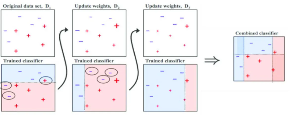
Gradient boosting machines (GBM) introduces the concept of boosting, but in its core they have

similarities with RFs. In fact, they also act as an ensemble. The term boosting is related to its major

advantage over RFs due to the fact that each tree (classifier) is trained on the last tree’s errors – Figure

12131. Datapoints which were mislabelled by the prior classifier are attributeda higher weight in the next

classifier’s training so the model will be more penalized when mislabelling these instances. This process is done iteratively which will eventually lead to a final model being trained in each classifier’s error. GBMs have gained a lot of attention in the last few years, being responsible for a large number of winnings in

Kaggle competitions132. In analytical chemistry, GBMs are mostly applied in classification problems

regarding high-dimension data133–135.

Figure 12 - Training of a gradient boosting machine. (adapted from ref 131)

Support Vector Machines

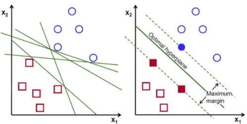
Support vector machine (SVM) is a supervised learner proposed by Vapnik in the nineties136_.

Although it can be applied in both regression and classification problems it is mainly applied in the latter. In classification tasks, the intuition behind it consist in defining a decision boundary that maximizes the distance between different classes – Figure 13.

Figure 13 - Intuition behind SVM hyperplane definition. (adapted from ref 136)

Since an infinite number of hyperplanes can be defined (Figure 13, left) SVMs take advantage of the closest datapoints from different classes to define the optimal decision boundary by using them to define support vectors to set the optimal hyperplane (Figure 13, right), i.e., the hyperplane which maximizes the distance between closest datapoints from different classes. When data is linearly separated without any mislabelled datapoints it consists in a hard margin SVM, the opposite constitutes

a soft margin SVM137.

SVM became popular in the nineties due to the cheap computation cost and the good performance it implied being broadly applied in topics as QSAR and drug design. Despite the fact that they are now outperformed by more flexible models, they are still applied in analytical chemistry mainly in classification tasks138,139_.

2.3. Bridging Analytical Chemistry and Machine Learning

While the first section of this chapter intended to present each step of the analytical chemistry process with a special focus on data interpretation and ML’s role in it, the second explored basic concepts regarding ML aiming to understand what it is and how it works. This third and last one aims to bridge

the first two. Its goal is to summarize how ML can be a valuable tool in analytical chemistry and to cover some recent applications regarding this interface.

2.3.1. Motivation and applications of Machine Learning in Analytical Chemistry

Analytical chemistry came a long way since 1860 when Bunsen and Kirchhoff developed the

first flame emissive spectrometer which allowed the discovery of the alkali metals rubidium and cesium140.

In the first half of the twentieth century occurred a revolution in the analytical instrumentation which widened the answers an analyst could gather from those analysis. With novel, upgraded, sophisticated techniques more and more information could be attained which required more complex ways in order to interpret what that information meant. Nowadays, modern analytical instrumentation generates so much data that it is now called megavariate data. All this chemical data brought up the need to implement new ways of examining it.

Simultaneously, social and technological advancements allowed the ordinary application of ML in several science fields including analytical chemistry. This interface where ML is applied in domains

such as particle physics141 and biology142 had already revealed very useful enabling several breakthroughs.

In chemistry, numerous areas have benefited from its application ranging from catalysis143,144_{, drug}

discovery105,145,146 _{to material science}147,148_{. Some AI experts even claim chemistry should be the next grand}

challenge for AI149_{. Among other things the authors argue the knowledge acquired in conventional AI}

studies such as two-player board games and human-mimicking tasks as nature language processing or computer vision, places AI community in a good position to tackle chemical challenges with incredible

benefitsfor humanity. In fact, complex chemical tasks as retrosynthesis are now capable of AI automation

with a performance at least as good as a skilled chemist150_{. In this study, Segler} et. al _{used Monte Carlo}

tree search and symbolic AI to propose retrosynthetic routes. By training DNNs on more than 12 million single-step reactions the authors developed an AI system capable of understanding the underlying rules

of retrosynthesis in such a way that in double-blind AB test, chemists considered the AI-generated routes to be equivalent to those reported in literature.

An increasing number of works have been done in the interface between chromatography

and ML. Cao et. al proposed an approach called quantitative structure-retention relationship (QSRR) to

predict the retention time of a compound given a chromatographic setup151_{. To attain this, the authors}

used a dataset of 93 molecules where molecular descriptors were used as features and its respective

retention times. In contrast with Segler et. al where DNNs were used, this work relies on RFs to build the

predictive model.

Recently, another interesting approach called quantitative pattern-pattern relationship (QPPR) was developed to predict the effect that firing a gun has in the chemical composition of the ammunition

constituents152_{. In forensic sciences, the association of the gunshot residue (GSR) to the person who took}

the shot constitutes a challenge for forensic experts. Traditional methodologies involve analysing the ammunition content, fire a gun and then analyse GSR from spent cases in order to establish a relationship between GSR and the original content. With QPPR, authors showed it was possible to relate GSR with the initial content without having to fire a gun using ML models. After testing 14 different learners, top performances were obtained with RFs and SVMs.

Considering quality control, ML has been successfully applied in egg authenticity153_{, adulteration}

of vegetable oils117,154 and citrus fruits’ quality155.

The ever-increasing number of works in this interface strongly indicates that, in the near future, having a basic understanding on how ML can be applied in analytical chemistry will be a valuable skill

Chapter 3 – Experimental

3.1. Implemented Methodology

In this chapter the employed methodologies as well as materials and software used in the development of this dissertation will be described.

The purpose of this project was to study how chemical data acquired from HPLC-MS can be used to attain useful insights regarding sample nature by applying ML tools. More specifically, the goal was to develop ML models able to classify PCBs according to four manufacturing conditions (MCs) by analysing the end product using HPLC-MS. Since ML models need significant amounts of data to train on, a novel data augmentation technique was developed alongside. The used analytical method was

performed according to IPC-TM-650 2.3.27.1157 _{whose objective is to analyse the chemical composition}

of PCB’s surface.

3.2. Samples

The selected samples for this study consisted in 180 PCBs manufactured under four distinctive conditions (A, B, C and D). There are 18 different combinations of PCB’s MCs – Figure 15. For each of those 18 different MCs there are 10 replicate samples produced under those same conditions with the exception of A1B3C1D1 and A1B3C1D2 which have 15 and five replicate samples, respectively. These 18 different groups are named according to the MCs that were used in their production (e.g.: a class can be represented as A2B1C2D2. This means conditions A2, B1, C2 and D2 were used during PCB production). For each MC there are two different possibilities except for condition B which has three possibilities (A1/A2, B1/B2/B3, C1/C2, D1/D2).

180 PCB

samples

Figure 15 - Diagram of the different manufacturing conditions used in PCB production as

3.3. Reagents

Acetonitrile was obtained from Fisher (Loughborough, UK); isopropyl alcohol (IPA) was purchased from Honewywell (Seelze, Germany). Both solvents were HPLC grade. Ultrapure water (18 MW.cm) was prepared using a Milli-Q Gradient A10 (Darmstad, Germany). Glacial acetic acid was purchased from Panreac (Barcelona, Spain).

3.4. Preparation of solutions

Extraction solution for SLE (IPA/water, 75:25 (v/v)) was prepared according to IPC-TM-650 in

1 L batches and kept in PTFE gallons in the dark at -4ºC. HPLC solvents were prepared individually by adding 500 mL of acetonitrile/water, sonicated in ultrasound bath for 30 min and added 0.1% (v/v) glacial acetic acid in the water shot.

3.5. Sample Preparation

SLE was performed according to IPC-TM-650 2.3.27.1 where PCBs samples were, additionally, cut in halves using a steel blade cutting machine, placed inside a KAPPAK SEALPAK #503 (VWR, USA) extraction bag, added 60 mL of the IPA/water extraction solution, heat-sealed the bag and placed inside a water bath at 75ºC for 60 min. After, the extraction bag was allowed to cool down to room temperature before opened, its extracted solution was transferred to 10 mL glass vials after filtered with a 0.2 mm PTFE filter. Extracted solutions were kept in the dark at -4ºC prior to analysis.

3.6. Instrumentation

Chromatographic separation was performed on an Kinetex RP-C18 (100x4.6mm, 2.6 µm) analytical column (Phenomenex, Torrance, CA). An Edwards E2M30 pump (Edwards, West Sussex, UK) was used for gradient elution at a constant flow of 0.3 mL/min.

HPLC solvents were: A (water, 0.1% acetic acid) and B (acetonitrile). The mobile phase was programmed as follows: original conditions 60% A, linear gradient to 10% A in 20 min, linear gradient to 60% A in 5 min. Re-equilibration time was 5 min.

Mass spectrometric measurements were performed on an LXQ (Finnigan, San Jose, CA) linear ion trap mass spectrometer equipped with an electrospray ionisation source (ESI) working in positive ion mode acquisition in a range from 50 to 1000 Da. The ESI parameters were: capillary temperature 250ºC, sheath gas flow 50 arbitrary units (a.u.), auxiliary gas flow 10 a.u., sweep gas flow 10 a.u., source voltage 5 kV, source current 100 µA, capillary voltage 10 V, tube lens 15 V, sheath gas nitrogen (Praxair, PT), auxiliary gas nitrogen (Praxair, PT).

3.7. Software and hardware

HPLC-MS files (chromatograms, MS spectra) were acquired and manipulated with the built-in software version of the equipment XCalibur Quant (version 2.7). Each analysis file is predefined exported in a RAW extension by the built-in software and converted to csv extension with a multi-group internally developed software. All data manipulation was performed with the following software: python v.3.6.8, imbalanced-learn v.0.5.0, matplotlib v.3.1.0, numpy v.1.16.4, pandas v.0.24.2, scikit-learn v.0.21.2, scipy v.1.3.0, seaborn v.0.8.1, xgboost v.0.90. Hardware specifications include: 2.3 GHz dual core Intel Core i5 CPU and 8 GB 2133 MHz LPDDR3 memory.

3.8. Data mining methodologies

Standard scaling was applied before data splitting. Training and test data were divided in 80/20 with class stratification. PCA, in the context of model development, was applied in preprocessing after scaling. The used features allowed to explain 95% of system’s variance which corresponds to 11 and 133 features regarding time and mass approach, respectively. Classifiers’ performances are measured by precision calculated according to equation 5.

Precision = True Positive

True Positive + False Positive (eq. 5)

All fifteen different classifiers were submitted to a 5-fold cross validation intending to evaluate model stability to data splitting. This is done by training five different ML models with different training sets and testing them in also five different test sets in an iterative process.

Chapter 4 – Results and Discussion

4.1. Overview

The role of data interpretation in the analytical chemistry process, currently constitutes one of the greatest challenges an analyst has to face. It involves understanding novel, advanced technology and concepts which until recently weren’t associated with analytical chemistry. In the past few years, ML have become such a valuable tool regarding this step that numerous works in this interface are now tackling interesting challenges in analytical chemistry. Hyphenated methods, such as LC-MS, are now capable of generating huge amounts of multi-dimensional data. This megavariate data contains much more information than the traditional data interpretation methods could explain which, as a consequence, gave rise to the application of ML tools in order to surpass this limitation.

This chapter is divided in two main parts. The first one presents results regarding laboratory work needed to guarantee the acquisition of high-quality chromatographic data whilst the second part shows results related to the development of ML models capable of predict MCs based on the previously acquired data.

Since this work supports confidential status, results are presented in a generalist, non-specific style aiming to show how the developed tool can be of interest to the analytical chemistry community rather than the problematic which was studied. Also, it is not the scope of this dissertation to study the chemistry of PCBs. Moreover, the confidential details are not relevant for the presented study and, for that reason, this chapter focus on the developed methodology.

4.2. Optimization of the analytical method

This section introduces the work carried on in order to guarantee high quality chemical data.

Since the analytical conditions of the employed method were already fine-tuned for a similar problem158

the intention with this first section is to guarantee that the analytical method, specifically the analytical conditions regarding separation, produce chromatograms in a suitable shape and quality to further fed ML algorithms in order to build predictive models for MCs.

4.2.1. Chemical Analysis – HPLC-MS

Efforts towards guaranteeing a suitable chemical profile capable of capture sample’s chemical

nature were made by testing three different analytical conditions as described in Table 4. Since no

methodologies for analytical method validation aiming to build predictive ML models were found in literature, the idea behind these tests is to ensure that the employed separation conditions allow a suitable peak separation and that no sample carryover occurs.

Condition Analytical

column Separation conditions

Flux (mL/min) 1 Kinetex C18 (100x4.6mm, 2.6 µm)

original conditions 60% A, linear gradient to 10% A in 20 min, linear gradient to 60% A in 5 min. Re-equilibration time was 5 min

0.3

2

Kinetex C18 (100x4.6mm,

2.6 µm)

original conditions 20% A, linear gradient to 10% A in 20 min, linear gradient to 20% A in 5 min. Re-equilibration time was 5 min

0.3

3

Luna C18 (100x2mm,

3 µm)

original conditions 60% A, linear gradient to 10% A in 20 min, linear gradient to 60% A in 5 min. Re-equilibration time was 5 min

0.25

In order to qualitatively evaluate the produced chromatograms a notation of peaks correspondent to ions at m/z 280 and m/z 375 were kept in each chromatogram (Figure 16) with the aim of assessing the degree of peak separation that is achieved with each condition presented in Table 4. Condition 1 (black, top) represents the analytical condition which is the base of the analytical method whilst conditions 2 (red, middle) and 3 (green, bottom) were presented for comparison purposes.

Figure 16 shows the resulting chromatograms of the three analytical conditions tested. Condition 3 indicates the employed separation conditions have a higher elution strength which results in a myriad of compounds being eluted in the beginning of the analysis thus decreasing peak separation and, subsequently, the quality of the chemical data. This information is also supported either by the large peak intensity observed in this condition which might happen as a result of having a large number of compounds being eluted at the same time as well as by the relative position of ions m/z 280 and m/z 375. In te n si ty 3 m/z 280 m/z 280 m/z 280

Figure 16 – Chromatograms of the tested analytical conditions. Ions at m/z 280 and m/z 375 are

denoted as references for peak separation evaluation. m/z 375

m/z 375

Condition 2 denotes a condensed chemical profile and a larger elution strength than the one required to produce an adequate peak separation. This information is also supported by the position of ion m/z 375. Although condition 2 arguably denotes the best peak separation regarding the beginning of the analysis, peak separation at mid-time analysis is slightly worst when compared with condition 1. Furthermore, due to the nature of the analytical setup, species eluted at the beginning of the analysis (solvent and unretained species) are more likely to be less important to the matter of classification when compared with mid-time analysis.

Thus, these results show the analytical conditions employed produce chromatograms with a suitable shape and quality for the desired end.

4.3. Machine Learning Model Development

In this section will be presented the obtained results regarding ML model development. The first subsection explores the obtained chemical data and introduces how the problem will be addressed by, regarding two different approaches. Second and third subsections focus on results related to each approach.

4.3.1. Exploratory Data Analysis

Each chromatographic analysis consists in a series of MS scans (ca.12k) which can be viewed

as a 30-min chromatogram. Figure 17(a) shows the total ion current (TIC) chromatogram of each MS spectra and Figure 17(b) depicts a MS spectrum related to the highest intensity peak at 18.93 min.

When this information is resumed in a tabular format, the same can be viewed as in Figure 18. Each column represents the measured intensity of ions ranging from 50 to 1000 Da and each row consists in a time series of the acquired MS spectrum.

Figure 18 - HPLC-MS data from the analysis of one PCB sample resumed in a tabular format.

Features include the ion intensity from 50 to 1000 Da in a time series where each row consists in a scan.

11_b2018_01HAc_pos #7746RT:18.93AV:1NL:3.39E6

T:ITMS + c ESI Full ms [50.00-1000.00]

100 200 300 400 500 600 700 800 900 1000 m/z 0 500000 1000000 1500000 2000000 2500000 3000000 In te n si ty 361.12 378.09 383.36 515.41 420.74 315.26 259.15 215.14 471.35 531.42 604.59 649.29695.21 751.62 187.28 789.91 846.54893.87942.70 140.15 RT:0.00 - 30.00 0 2 4 6 8 10 12 14 16 18 20 22 24 26 28 Time (min) 0 1000000 2000000 3000000 4000000 5000000 6000000 7000000 8000000 9000000 10000000 11000000 12000000 13000000 14000000 15000000 In te n si ty 18.93 19.00 2.87 2.72 12.05 18.81 12.21 5.38 2.99 5.32 21.24 18.74 12.45 3.084.945.56 21.30 5.78 11.90 _20.99 6.69 10.45 18.61 21.46 23.92 23.02 10.58 13.56 20.65 10.34 17.65 _24.07 6.83 10.08 10.67 19.33 13.70 17.24 7.05 7.54_9.539.97 13.77 15.58 24.30 _27.38 24.4427.01 27.60 0.99 NL: 1.52E7 TIC MS 11_b2018_ 01HAc_po s (b) (a)

Figure 17 – TIC (a) chromatogram and (b) MS spectrum for the peak at 18.93 min, acquired with the

To develop the ML model two different approaches regarding the used features were taken. One consisted in using the sum of TIC intensities – time approach. The second consisted in view each sample as the sum of ion intensities – mass approach. The objective with creating models using these two approaches is to compare both and to evaluate which one allows better ML model performances. The following subsections will present the results regarding both approaches.

Considering time approach, Figure 19 shows chromatograms of five independent replicate samples, where a similar chemical profile can be observed across all samples. Slight variations in peak shape and

area are expected as described in literature159. These can be related with some HPLC components

(detector, column, autosampler) but the main reasons are usually pressure and autosampler variations. Furthermore, for this approach the number of scans was reduced 100 times (from 12k to ca. 120). This way, noise can be reduced to improve model performance while still keeping the chemical information.

Figure 20 depicts the 20 highest intensity ions regarding three independent replicate samples. At this point, it is crucially to understand that peak intensity variations in mass approach are expected as a result of the ESI-MS detection setup that allows a nominal mass precision which in turn enables the

Time (min)