Licenciatura em Ciências da Engenharia Biomédica
Analysis of functional Magnetic Resonance data
for neurosurgical planning: subject specific
resting state analysis as a complement to task
based analysis.
Dissertação para obtenção do Grau de Mestre em
Engenharia Biomédica
Orientador: Alexandre Andrade, Doutor,
Instituto de Biofísica e Engenharia Biomédica, Faculdade de Ciências da Universidade de Lisboa
Júri
Presidente: Doutora Carla Maria Quintão Pereira
subject specific resting state analysis as a complement to task based analysis.
Copyright © Vera Rita Costa Salgado, Faculdade de Ciências e Tecnologia, Universidade NOVA de Lisboa.
A Faculdade de Ciências e Tecnologia e a Universidade NOVA de Lisboa têm o direito, perpétuo e sem limites geográficos, de arquivar e publicar esta dissertação através de exemplares impressos reproduzidos em papel ou de forma digital, ou por qualquer outro meio conhecido ou que venha a ser inventado, e de a divulgar através de repositórios científicos e de admitir a sua cópia e distribuição com objetivos educacionais ou de investigação, não comerciais, desde que seja dado crédito ao autor e editor.
Este documento foi gerado utilizando o processador (pdf)LATEX, com base no template “unlthesis” [1] desenvolvido no Dep. Informática da FCT-NOVA
First of all, I would like to thank the Institute of Biophysics and Biomedical Engineering (IBEB), where this dissertation was conducted, for all the support provided during this time.
I want to express my deepest gratitude to my supervisor, Alexandre Andrade. His guidance, support and availability were crucial for the success of this project. I am sincerely thankful for all the knowledge and experience achieved working with him.
I would also like to thank Dr. Martin Lauterbach, for the attentiveness and valuable contribution to this study.
To my parents, Cristina and José, I would like to say how grateful I am for all the emotional support and encouragement, not only in the last few months, but during my whole life. Thank you for the values that you transmitted, they are now far more treasured than ever. With the same gratitude I also would like to mention my brother, Francisco, for being supportive in his funny, but lovely way, and to my grandmother for all the knowledge and for being a role model my entire life.
To all people whom I shared my workspace with, I am thankful for all the assistance, dedication and companionship. Without you my lunch time would be certainly shorter but I wouldn’t have so many memorable moments to share. I thank each and every one of you for helping me in different occasions, giving me the support I needed and for
making this experience a remarkable one.
I also should not forget those who joined me in my academic journey. Your compan-ionship will not be forgotten.
Finally, I would like to thank my hometown friends, the ones that I grew up with. Thank you for understanding my absence during the last 5 years. I know you are, as you always have been, rooting for my success.
Brain and other central nervous system tumors are the 17th most common cancer type in Europe, being associated with high mortality rate. Neurosurgery has been the ultimate solution for the treatment of brain tumors. Integration of preoperative brain mapping in the process is highly recommended in order to preserve fundamental areas of the brain, especially those believed to be connected to language and movement. Recently, there has been a growing interest in presurgical planning resorting to resting-state functional magnetic resonance imaging (fMRI).
The aim of this thesis is to explore strategies to process data of resting-state fMRI in order to better understand its connection to task brain networks, and to assess their application to the protocols currently used within clinical institutions that are partners of the host scientific institution in an ongoing project. A total of 8 subjects were re-cruited to participate in this study, all of them previously referred for surgical tumor resection. An optimal strategy for pre-processing was devised and tested. Task data was processed using the General Linear Model, while rest data was processed through Inde-pendent Component Analysis. The processed data were then correlated via similarity coefficients.
The results of similarity tests show a limited coincidence between resting-state net-works and the activation task areas. Further studies will be required in order to improve these results.
Os tumores cerebrais, juntamente com outros tumores do sistema nervoso central são o 17º tipo de cancro mais comum na Europa, estando associados a uma elevada taxa de mortalidade. A neurocirurgia tem sido uma das soluções para o seu tratamento. Neste âmbito, a integração do mapeamento cerebral pré-cirúrgico no processo é altamente recomendada a fim de preservar áreas fundamentais do cérebro, nomeadamente as que estão relacionadas com a linguagem e com o movimento. Recentemente, tem havido um crescente interesse no planeamento pré-cirúrgico com recurso à imagem de ressonância magnética funcional em repouso.
O objetivo desta tese é explorar estratégias para processar dados de ressonância magnética funcional em repouso, com o intuito de compreender a sua relação com re-des cerebrais provenientes de paradigmas de tarefa, e explorar a aplicabilidade re-dessas estratégias nos protocolos actualemnte usados nas instituições clínicas associadas à ins-tituição de acolheminto, no contexto de um projecto em curso. Um total de 8 indivíduos foram recrutados para participar neste estudo, todos eles previamente referenciados para resseção cirúrgica do tumor. Foi concebida e testada uma estratégia otimizada para o pré-processamento. Os dados de tarefa foram processados utilizando o Modelo Linear Geral, ao passo que os dados de repouso foram processados através da análise de com-ponentes independentes. Os dados processados foram posteriormente correlacionados através de coeficientes de similaridade.
Os resultados dos testes de similaridade mostram uma coincidência limitada entre as redes de repouso e as áreas de ativação provenientes de paradigmas de tarefa. Serão necessários mais estudos de forma a melhorar estes resultados.
List of Figures xv
List of Tables xvii
Acronyms xix
1 Introduction 1
1.1 Objectives . . . 2
1.2 Dissertation overview . . . 3
2 Background 5 2.1 Brain Tumors - Basic Concepts . . . 5
2.1.1 Eloquent Areas . . . 6
2.2 Surgical Planning . . . 7
2.2.1 Brain Imaging Techniques . . . 7
2.2.2 Magnetic Resonance Imaging . . . 9
2.2.3 Resting State functional Magnetic Resonance Imaging . . . 11
2.2.4 fMRI processing . . . 14
3 Materials and methods 21 3.1 Participants and Image acquisition . . . 21
3.2 Preprocessing . . . 23
3.3 Processing . . . 28
3.3.1 Task data - Statistical Analysis . . . 28
3.3.2 Rest data processing . . . 32
3.4 Comparison of Task Networks and Resting State Networks . . . 33
4.1.1 Scrubbing . . . 37
4.1.2 Normalization . . . 38
4.1.3 Removal of nuisance signals . . . 40
4.2 Intra-Subject Analysis . . . 41
4.2.1 Motor Paradigms . . . 41
4.2.2 Language . . . 56
4.3 Intra-Task Analysis . . . 64
4.4 Results Overview . . . 72
5 Discussion 73
6 Conclusion 77
2.1 Classic anatomic sites for functional brain areas . . . 13
2.2 Resting-State networks . . . 14
3.1 DPARSFA layout . . . 24
3.2 DPARSFA options . . . 27
3.3 SPM layout . . . 29
3.4 fMRI model specification . . . 30
3.5 GIFT layout . . . 33
3.6 GIFT options . . . 34
3.7 The overall scheme . . . 36
4.1 Difference between normalize and not normalize images . . . . 39
4.2 Effect of nuisance signals removal . . . . 40
4.3 Mouth activation map for Sub003 . . . 42
4.4 SPM environment . . . 44
4.5 Rest and task correlation map . . . 45
4.6 Independent Component of Sub003 rest network . . . 46
4.7 Hands activation maps for Sub003 . . . 49
4.8 Rest activation maps for Sub003 . . . 50
4.9 Feet activation maps for Sub003 . . . 52
4.10 Rest activation maps for Sub003 . . . 53
4.11 Syntactic Decisions activation maps for Sub003 . . . 57
4.12 Independent Component of Sub003 rest network that is more similar with the syntactic decision activation map . . . 58
4.13 Independent Component of Sub003 rest network that is more similar with the verb generation activation map . . . 60
2.1 Brain tumor classification . . . 6
3.1 Demographic features of the study population . . . 22
4.1 Scrubbing Results . . . 38
4.2 Similarity results for rest activation maps and mouth paradigm activation maps for Sub003 . . . 47 4.3 Similarity results for rest activation maps and mouth paradigm activation
maps for Sub003, with nuisance signals removal . . . 48
4.4 Similarity results for rest activation maps and hands paradigm activation maps for Sub003 . . . 51
4.5 Similarity results for rest activation maps and feet paradigm activation maps for Sub003 . . . 54
4.6 Similarity test results for rest activation maps and with the result of the superposition of the 3 motor tasks for Sub003 . . . 55
4.7 Similarity results for rest activation maps and syntactic decision paradigm activation maps for Sub003 . . . 59
4.8 Similarity test results for rest activation maps and verb generation paradigm activation maps for Sub003 . . . 62
4.9 Similarity test results for rest activation maps and with the result of the superposition of the 3 motor tasks for Sub003 . . . 63
4.10 Similarity test results for rest activation maps and hand activation maps for Sub001 . . . 64
4.11 Similarity test results for rest activation maps and hand activation maps for Sub002 . . . 65
4.13 Similarity test results for rest activation maps and hand activation maps for Sub004 . . . 67 4.14 Similarity test results for rest activation maps and hand activation maps for
Sub005 . . . 68 4.15 Similarity test results for rest activation maps and hand activation maps for
Sub006 . . . 69 4.16 Similarity test results for rest activation maps and hand activation maps for
Sub007 . . . 70 4.17 Similarity test results for rest activation maps and hand activation maps for
BET brain extraction tool.
BOLD blood oxygenation level dependent.
CNS central nervous system.
CSF cerebrospinal fluid.
DICOM Digital Imaging and Communications in Medicine.
DMN default-mode network.
DNA deoxyribonucleic acid.
DPABI Data Processing and Analysis for Brain Imaging.
DPARSFA Data Processing Assistant for Resting-State fMRI- advanced edition.
DSC Dice similarity coefficient.
ECS electrical cortical stimulation.
EEG electroencephalography.
FD frame-wise displacements.
fMRI functional magnetic resonance imaging.
FWE familywise error.
FWHM full width at half maximum.
GLM General Linear Model.
hrf hemodynamic response function.
IC independent component.
ICA independent component analysis.
MEG magnetoencephalography.
MNI Monreal Neurological Institute.
MRI magnetic resonance imaging.
NIfTI Neuroimaging Informatics Technology Initiative.
PC principal components.
PCA principal component analysis.
PET positron emission tomography.
ReML restricted maximum likelihood.
REST Resting-State fMRI Data Analysis Toolkit.
Rf Radiofrequency.
rs-fMRI resting state functional magnetic resonance imaging.
RSN resting state networks.
SMN sensorimotor network.
SN salience network.
SPM Statistical Parametric Mapping.
TE echo time.
TR repetition time.
C
h
a
p
t
1
I n t r o d u c t i o n
Tumors of the central nervous system are associated with a high incidence and mortality rate. In 2012, brain and other central nervous system cancer was reported to be the 17th most common cancer type and the 12th most common cause of cancer death worldwide. Neurosurgery has been the ultimate solution for the treatment of these pathologies, with really satisfactory outcomes [1]. Nevertheless, in those circumstances, integration of preoperative brain mapping in the process is highly recommended in order to preserve fundamental areas of the brain, especially those believed to be connected to language and movement, denominated eloquent areas, and reduce post-operative deficits [2] [3]. In this scope, the search for an accurate knowledge about the structure and func-tionality of the brain has been one of the most important challenges for pre-planning neurosurgery.
fMRI, as an innocuous approach, has proven to be a promising technique to acquire the activation sites of the human brain involved in the eloquent functions, through assess-ment of changings in blood oxygenation level dependence (BOLD) [3]. Typically, fMRI appraises small hemodynamic fluctuations induced by stimulus or by task performance [3] [6].
Nonetheless, recent developments led to the belief that there is a temporal and functional correlation among separated brain regions, responsible for behavioral and cognitive functions control, even in rest conditions. In addition, there are small changes in BOLD signal during rest that confirm an incessant interaction between brain net-works, thus leading to Resting-State Network [2] [3] [7]. Despite the increasing interest in this new approach, there is still a long way ahead until resting-state fMRI is com-pletely accepted and applied inside the clinical realm [8].
1.1 Objectives
The aim of this thesis is to explore strategies for resting-state fMRI data processing in order to better understand its relationship with brain networks from task paradigms and its contribution in improving diagnosis and pre-surgical planning. As a result, subjects unable to perform tasks, such as asleep or anesthetized patients, could benefit from this diagnostic technique, since it does not require the performance of any task. For this purpose, it is intended to test and optimize a preprocessing protocol, followed by the adaptation of some processing protocols used in the literature, devised for the task and rest data individually. Finally, it is intended to employ the results from these procedures in similarity analysis, aiming to realize the resemblance between brain activation in task performing and at rest, in order to test the reliability of resting state data analysis to complement the classic task approach in pre-surgical planning.
1.2 Dissertation overview
This section aims to present a brief description of topics covered in each chapter in order to provide an enlightened reading.
Chapter 2. Backgroundreviews the background literature related to the work de-veloped in this dissertation. In particular, it provides some basic concepts about brain tumours, such as the brain mapping methodologies commonly used for surgical plan-ning, which includes a description of functional magnetic resonance imaging ant its newest approach, resting state fMRI.
Chapter 3. Materials and methodsdetails how the current study was conducted, undergoing a brief exposition of the software and methodology implemented. It also presents a brief description of the participants and the image acquisition protocol, fol-lowed by the detailed information about the methods and software used in the prepro-cessing and proprepro-cessing stages Finally, it is explained how the task based and resting state maps were superimposed such as its correlation calculation.
Chapter 4. Results intends to report the most relevant results obtained in pre-processing and pre-processing stages, followed by the presentation of statistical and simi-larity analysis results.
Chapter 5. Discussionpresents the analysis and discussion of the study results, as some limitations and suggestions for improvement.
C
h
a
p
t
2
Ba c k g r o u n d
2.1 Brain Tumors - Basic Concepts
The human brain composes the central nervous system (CNS) along with the spinal cord and meninges. Taken together, they are responsible for controlling the majority of the bodily functions [9]. As with all other parts of the body, the CNS comprises nu-merous cells some of whose functions are managed by the deoxyribonucleic acid (DNA) , which is contained in their nuclei. When DNA carries a disability these functions may be compromised. More specifically, mutation of DNA can affect the production,
growth and division cycle of cells, leading to an abnormal mass accumulation which compresses and damages the surrounding brain areas, commonly named as brain tumor or intracranial neoplasm [10].
Brain tumors are highly variable in shape, size and localization.They can be catego-rized as primary or metastatic. The first group refers to an abnormal mass that arises originally from the brain, whereas the second one refers to tumors that begin outside the CNS and then spread to the brain, such as metastasis from breast, lung and kidney cancer [11].
Brain tumors have their designations by the location in which they begin. Some of these are listed in table 2.1.
Table 2.1: Brain tumor classification [12] [13] [14]
Brain Tumors Classification Localization
Primary Brain
Tumors
Gliomas
Astrocytomas Glial cells - astrocytes. Most often in the cerebrum
Oligodendrogliomas
Cells that make the fatty substance that covers
and protects nerves.
It usually occurs in the cerebrum
Ependymomas Cells that line the ventricles or the central canal of the spinal cord.
Primary cerebral lymphoma Lymphatic system
Choroid plexus papillomas Producer cells of cerebrospinal fluid, which are located in the ventricles.
Haemangioblastomas Posterior cranial fossa.
Metastatic tumors Another part of the body, such as lung, breast or kidney.
Meningiomas Meninges.
Cranial nerve schwannomas Supporting nerve cells called vestibular schwannomas
Pituitary adenomas Pituitary gland, that is located at the base of the brain.
to slow or stop the growth of the tumor;b)chemotherapy, that relies on the use of drugs to destroy cancer cells, usually by stopping the cancer cells’ ability to grow and divide; andc)surgery, which includes complete or partial tumor resection [11] [15].
As a matter of fact, neurosurgery has been the ultimate solution for a number of subjects with brain tumors with really satisfactory outcomes[15]. Among other brain tumors, gliomas and metastases represent almost 60 % of brain tumor surgery, while meningiomas account for 20% and schwannomas and pituitary adenomas for 15% [12].
2.1.1 Eloquent Areas
human brain is necessary for the presurgical planification. Damage to these areas gen-erally leads to major neurological deficits. Brain areas responsible for motor function are mostly located in the precentral gyrus just anterior to the central sulcus. However, there are several other areas that are likewise relevant to body motion. Premotor and supplementary motor area include brain regions responsible for planning and control-ling movement. Both of those areas are located in the mesial and lateral side of superior frontal gyrus, forward to precentral sulcus. The communication of those different areas
throughout the corticospinal fiber tract is responsible for coordination and synchronic-ity of movements. [16].
Sensorial information follows the inverse pathway of motor function and it is mainly directed to the primary somatosensitive area, located in the postcentral gyrus, posterior to the central sulcus [17] [16].
Broca’s area, believed to be one of the areas responsible for speech production, is anatomically located in the inferior frontal gyrus and it is composed by two areas: the pars triangularis and the pars opercularis. The function of Broca’s area is to command the muscles so that they produce meaningful sounds. Broca’s area is connected to Wernicke’s area through a white-matter fiber tract called arcuate fasciculus. Wernicke’s area is one of the areas responsible for language understanding. It’s placed on the back portion of temporal lobe of the dominant hemisphere, that generally is the left hemisphere [17].
2.2 Surgical Planning
The challenge of brain lesions’ surgical resection is balancing the aim of maximizing resection with the requirement to preserve functionally-relevant brain areas, especially those believed to be connected to language and movement, denominated eloquent ar-eas[16]. In this scope, accurate localization of those areas is essential for presurgical planning, as it helps optimize resection and decrease postoperative deficits [18] [6] [3].
2.2.1 Brain Imaging Techniques
subjects led to a growing concern to develop new imaging techniques capable of creating individual brain maps.
The first subject specific’s functional mapping procedure was an extremely invasive technique, called Intracarotid Amobarbital procedure or Wada Test. During this intra-operative method, an anesthetic medication is injected into the right or left internal carotid artery putting that hemisphere to sleep and incapable to communicate with the opposite side [18]. The main goal of this procedure was to determine which side of the brain controls language function and how significant each hemisphere is in regard to memory function [20].
The Wada Test has been replaced or complemented by electrical cortical stimulation (ECS), another invasive procedure that resorts on stimulation of the cerebral cortex’s surface while the patient is awake and performing motor, language or cognitive con-trolled tasks. This approach can only be used in intra-operatively stage and as it relies on the use of anesthetics it may produce unsatisfying outcomes [6] [20].
Regardless of whether the Wada Test or ECS are considered the gold standard pro-cedures for mapping brain function, both require an awake and cooperative subject. Their invasive nature led to the need for non-invasive approaches. With the advent of high resolution non-invasive neuroimaging, there has been improved ability to map the structure of the brain, as well as its connections. In this scope, techniques such as fMRI, electroencephalography (EEG), magnetoencephalography (MEG) and positron emission tomography (PET) have been adopted in order to trace network connections that are subject-specific and therefore to provide profitable information for pre-surgical planning assessment [5] [2].
In a brief description, PET is based on the detection and imaging of positron-emitting radionuclides that were previously administrated to the patient. PET images demonstrate indirectly functional courses involved in cerebral metabolism. Like other techniques, such as computed tomography or magnetic resonance imaging (MRI), PET relies on reconstruction tecquniques to obtain tomographic images. In order to acquire better anatomic localization of the regions of interest PET images can be overlaid with anatomic images such as MRI or computed tomography [21].
As for the EEG, it is a direct measure of brain function which records the electrical activity of the brain resorting to electrodes that are placed on the subject’s scalp. The time-series of scalp potential maps represent the differences in electric potential of
distinct brain areas [2] [22].
These magnetic fields are generated by neuronal electrical currents. The spatial dis-tributions of the magnetic fields are analyzed in order to map brain regions involved in specific functions. Since the magnetic field measured by MEG is produced directly by electrical neuronal activity, it is possible to detect signals from the brain on a sub-millisecond time scale [23].
Although all brain mapping techniques should present identical outcomes, inter-modal variations exist.
2.2.2 Magnetic Resonance Imaging
MRI is an imaging technique that relies on protons and their inherent magnetism to generate an image. As the human body is composed mainly of water, MRI takes ad-vantage of the great abundance in hydrogen nucleus (¹H) by manipulating them with Radiofrequency (Rf) energy in the presence of a strong magnetic field [24].
The hydrogen atom consists of an orbiting electron and a single positively charged proton (nucleus) which spins around its axis, creating a magnetic moment along the direction of spins’ axis. The sum of all the magnetic fields of each spin is called net magnetization. In the absence of an external magnetic field, the nuclei of hydrogen atoms in a sample are randomly distributed and therefore the sum of all the results in a null net magnetization. On the other hand, when exposed to a strong static magnetic fieldB0, the nuclei will align parallel or anti-parallel to the field. As it requires less energy, the majority of the spins allign parallely with fieldB0creating a magnetization in that direction. The nuclei precess with an angular frequency determined by the Larmor frequencyω0. The relation between Larmor frequency and the main magnetic field strength is displayed in the equation 2.1, where ψ represents the gyromagnetic ratio. Nevertheless, not all spins rotate in the same phase, therefore the sum of all the spins’ transverse magnetizations is null.
ω0=ψ·B0 (2.1)
Longitudinal relaxation corresponds to exponential recovery in longitudinal mag-netization. It is characterized by the energy exchange between the spins and the sur-rounding environment. The recovery rate is a constant tissue-specific time generally called T1. On the other hand transversal relaxation is result of a progressive dephasing of nuclei following the RF pulse caused by a spin-spin interaction. This inter-dipole interaction time is an exponential decay in transversal magnetization and is designated by T2. The MRI ability to create anatomic images is due to the tissue-specific relaxation times, which enables the differentiation between different tissues.
In actual MRI procedures, the transversal relaxation time is shorter than T2. The in-consistency results from the inhomogeneities in the main magnetic field. This observed time, called T2∗, has an essential role on functional Magnetic Resonance Imaging.
2.2.2.1 Functional Magnetic Resonance Imaging
In the last 25 years, the neuroimaging world had suffered several great updates and
innovations. The discovery that MRI could be sensitive to brain activity, besides its anatomy, was probably the most remarkable one [25].
In regular brain imaging techniques the main goal is to distinguish different tissue
types. Nonetheless, in functional brain imaging the purpose is to assess signal fluctua-tions over time. fMRI is one functional neuroimaging technique used to measure brain activity [26].
When a specific brain region increases its activity due to a task or a stimulation, the initial amount of oxygenated haemoglobin in the nearest blood vessels decreases, enhancing the deoxygenated haemoglobin. Seconds passed, there is a demanding need for additional oxygen and thus the blood flow increases, providing a great amount of oxygenated haemoglobin. fMRI is sensitive to this expansive rebound and the relative decrease in deoxyhemoglobin concentration, as it introduces a low increment inT2∗ weighted signal. This phenomenon is called blood oxygenation level dependent (BOLD).
The basic foundation of fMRI is the fundamental difference in the paramagnetic
properties of deoxygenated and oxygenated haemoglobin. The hemoglobin molecule has magnetic properties that differ whether it is bound to oxygen or not. The oxygenated
hemoglobin (Hb) has no unpaired electron and no magnetic moment (diamagnetic), therefore it is not magnetically distinct from other tissues. In contrast deoxyhemoglobin (dHb) has an unpaired electron and magnetic moment (paramagnetic) and thus deoxy-genated blood differs in its magnetic properties from surrounding tissues [27].
ionizing radiation-free technique, fMRI can assess brain function safely. Besides, due to its good spatial resolution, fMRI has been broadly used in clinical settings. Alongside the pre-surgical planning, the use of this functional imaging method has played a key role in functional evaluation in brain tumor management [28], in the study of Parkin-son’s disease [29], as well as in early detection of Alzheimer’s disease [30], and also in investigations of psychiatric disorders such as schizophrenia and severe depression [28]. More specifically, in pre-surgical context, fMRI demonstrates great precision in defining which hemisphere is language dominant, helping to decrease post-operative deficits, likewise reducing surgical time and improving the decision of the areas to recess.
Recent studies on spontaneous modulations in BOLD signal revealed the repro-ducibility of traditional fMRI in the absence of stimuli. These advances mean a new range of applications and prospects of fMRI and this topic will be explored in the next section.
2.2.3 Resting State functional Magnetic Resonance Imaging
strongest correlations were between the left and the right sensorimotor cortices [35]. Later studies confirmed the existence of synchronous fluctuations between other func-tional networks, like the primary visual network, auditory network and higher order cognitive networks [35] [36]. Biswal, in addition, showed that resting-state and task-based activation maps are notably similar [35]. These low frequency BOLD fluctuations observed while in resting show temporal correlations between anatomical distinct areas of the brain. These patterns have been designated "intrinsic connectivity networks" or "resting state networks".
Since initial contributions of Biswal up to the present day, the study of resting-state networks has shown a huge potential for the diagnosis of several pathologies like Alzheimer’s, miultiple sclerosis, autism, Tourette syndrome among others [8].
Although the true origin of these resting state BOLD signal oscillations (∼0.01− 0.1Hz) is not fully understood yet, it is proven that they are intrinsically generated by the grey matter and are not consequence of external stimulation.
2.2.3.1 Resting State Networks
The discovery of brain’s resting state networks was accidental. Scans of resting-state brain started to be included in the task-paradigm studies as a baseline for comparison. However, investigators noticed that some brain regions were more active in resting conditions than in controlled task .
The first resting state network to be discovered was default-mode network (DMN). The default mode network, is a group of brain regions that shows higher levels of activity when the subject is not involved in any mental exercise. This network is responsible for memory consolidation, monitoring the environment, keeping awareness even when resting and other ongoing intrinsic thoughts. Anatomically, the regions involved on this network are generally the medial prefrontal cortex, posterior cingulate cortex, and the inferior parietal lobule. Other regions as the lateral temporal cortex, hippocampal formation, and the precuneus are also described in literature as being included in DMN [37]. For an enlightened interpretation consult figure 2.1.
Several other resting state networks (RSN) have been studied and described in liter-ature. Although there is no concordance on names or localizations, there are 4 major resting-state networks in addition to DMN: auditory, visual, salience and sensorimotor network, see figure 2.2. Hereinafter are a brief description of them.
auditory network enfolds transverse temporal gyrus, also known by Heschl’s gyrus, that contains the primary auditory cortex (Brodmann area 41), and also bilateral superior temporal gyri, and posterior insular cortex [38] [39].
Visual network can be decomposed in three sub-networks. The medial visual net-work is responsible for simple visual task, while lateral and occipital visual netnet-work is believed to be incorporated in high-order visual and emotional stimuli [38]. The visual network encompasses most of the occipital cortex [40].
The salience network (SN) consists of three main cortical areas: the dorsal anterior cingulate cortex, the left and anterior right insula (aRI), and the adjacent inferior frontal gyri. It is believed that SN is involved in coordination of behavioral responses, including switches between intrinsic attention (DMN) and task-related states, cognitive control and implementation of repeated tasks [38].
The sensorimotor network (SMN) is responsible for preparing the brain to perform a coordinated motor task. This specific network is anatomically divided into motor and sensory cortices. The primary motor cortex covers a region that starts in the bottom of the precentral sulcus and extendens to the bottom of the central sulcus, whereas the primary sensory area covers the bottom of the central sulcus up to the bottom of the postcentral sulcus [39], extending to the supplementary motor areas [38].
Figure 2.2: Resting-State networks [38]
2.2.4 fMRI processing
Branco et al. (2016) and Tie et al. (2014) [42] [43] [44] focus on the study of language tasks maps and its similarity to rest maps. In all these studies, the methodology used for task image processing differs from resting images processing. In the first case, a
clas-sical approach to General Linear Model is used to extract the activated regions, whereas the second one is based on independent component analysis. Contextualization and information of these methods are described in the following sections.
2.2.4.1 Task: Statistical analysis and General Linear Model
General Linear Model (GLM) is a statistical linear model that aims to predict the varia-tion of the dependent variables through a linear combinavaria-tion of several model funcvaria-tions plus error. The general linear model is a generalization of multiple linear regression model altough with more than one dependent variable.
In fMRI context, the dependent variables represent the time course of each voxel,
Y, while the regressors, or predictors, that compose the design matrix correspond to time courses of what is believed to be fMRI responses towards tasks or head movements, equation 2.2. Each regressorX has an associated coefficient,β, which weights its
con-tribution on the voxel time course Y. It is then necessary add an error value,ǫ, to offset
noise fluctuation. That value is a random variable that is assumed to have a normal distribution of mean zero and variance valueσ2, equation 2.3. In every design matrix the first column, or the first regressorx0, is constant and equals to 1. Its corresponding
β0value is the signal at the starting conditions and it helps to model the main effect for the repeated measure factor on responses.
y1= β0x0 + β1x11 + ··· + βpx1p + ǫ1
y2= β0x0 + β1x21 + . . . . + βpx2p + ǫ2
..
. ... ... ... ... ...
yn= β0x0 + β1xn1 + ··· + βpxnp + ǫp
(2.2)
ǫ∼N(0, σ2) (2.3)
(equation 2.4) . y1 y2 .. . yn =
1 X11 ··· ··· X1p
1 X21 ··· ··· X2p ..
. ... ··· ··· ...
1 Xn1 ··· ··· Xnp
x β0 β1 . βp + ǫ1 ǫ2 .. . ǫn (2.4)
In order to assess if the hypothetical fMRI task responses correspond to real brain activations, GLM performs statistical data analysis.
Statistical data analysis allows to compute the difference among task activations and
rest periods, comprising the amount of variability of the measured data points,i.e, the amount of noise fluctuations. Thus, assuming the null hypothesis, the probability of a randomly activation has occurred can be calculated.
A t-test is one of the statistical hypothesis tests that estimate the uncertainty of an activation. It describes the relationship between the mean of the observed difference of
two effects (for example, activation and rest) with the variance of the noise fluctuations
from the data, equation 2.5.
t= X2−X1
ˆ
σX2−X1
(2.5)
For data with large noise fluctuations, the value oft is small, or in contrast, the higher thet value, the greater the likelihood that the observed mean difference is result
of a true activation.
Thep-value helps to determine the significance of the results. It represents the prob-ability that the observed spatial pattern was created by some random process. Which means that ifpis low, the observed mean difference exists, or in other words, it means
that the activation occurred.
5000 false positives. Therefore, it is common to correct thep-threshold - familywise er-ror (FWE) correction. The FWE relies on the fundamentals of Bonferroni correction, but taking into consideration the spatial correlation between voxels, since the Bonferroni correction, which assumes statistical independence between the multiple tests would be too strict [45]. There are other correction approaches such as voxel-wise control of the false discovery rate and formal heuristics.
A different solution is apply a lower uncorrected threshold. A typical threshold is
p <0.001. This threshold may be too conservative and thus produce false negatives.
2.2.4.2 Resting-state fMRI data processing
Several techniques have been suggested to process resting state functional magnetic resonance imaging (rs-fMRI). Although these techniques have distinct methodological basis they can be distinguished into two major groups: dependent and model-free methods.
1. Model-dependent method: seed method
Andrews-Hanna [46], Biswal [35], Cordes [36] and their respective colleagues studied functional connectivity applying seed-based methods. These techniques consist of correlating the resting-state time-series of a specific region of the brain against the times-series of all other brain’s regions. The selected region is typically called seed and can be defined based on activation maps or anatomically, from an atlas. The result is a functional connectivity map defining the functional connec-tions of the predefined seed. In spite of being a simple technique, the seed based approach only provides information of the functional connections of the selected region of interest [40] [47]. Instead of correlation, more sophisticated association measures can be used, such as coherence.
2. Model-free methods
Clustering strategies intend to gather variables with high level of similarity. There-fore, clustering outcomes may be more similar to traditional functional connectiv-ity maps and consequently simpler to understand. Several clustering algorithms have been described. Hierarchical clustering, k-means and c-means algorithms are some of the most talked about in the literature [48] [49].
In contrast to the above mentioned method, PCA attempts to identify a reduced number of uncorrelated variables from a large set. These incoherent variables are usually designated as principal components (PC). The first PC reflects the linear combination of the components with highest variance and the following ones are the orthogonal components of the previous. PCA reveals the greatest amount of data’s variance with the fewest number of PC [50]. PCA was used in studies headed by Friston [51] and Damoiseaux [52].
Lastly, ICA has been used in studies headed by Kiviniemi [53] and Beckmann [54]. The goal of this method is to search for sources of brain signal that are maximally independent from each other in order to separate spatial or temporally independent patterns from linearly mixed BOLD signals. One advantage of ICA has upon the seed approach is its aptitude of removing physiological and motion artifacts. The fundamentals of ICA are described in subsection 2.2.4.3.
2.2.4.3 Independent Component Analysis
fMRI datasets are composed by combinations of several physiological and external sig-nals produced by different sources. Extracting the signals of interest is a big challenge
once the signals are not static and could vary in space and over time. Independent Com-ponent Analysis (ICA) is one statistical technique for decomposing a complex dataset into subcomponents. It was first described by Comon in 1994 and it has been applied in many different fields. To better understand the theoretical design of this method
it is common to resort to a cocktail party analogy. In a cocktail party, microphones are placed indistinctly over the room. Each microphone records a different signal, that
results from the distance from each source, which in this example are the conversa-tions and the music band playing. What ICA proposes to do is to decompose the signal recorded by each microphone into its different sources. Similarly, ICA has the same
Mathematically, one can describe ICA using the following vector-matrix notation (equation 2.6).
x=A·s (2.6)
Wherexcontains the observed (mixed) signals,sis a two-dimensional random vec-tor containing the independent source signals andAis the two-by-two mixing matrix. This algorithm can be described as a statistical “latent variables” model because the independent components and the mixing matrix cannot be directly observed, unlikex. Then ICA tries to find a linear transformation at the feature space x into a new feature spaces, where each of the individual new features are mutually statistical independent and the mutual information from the new space and the original one is high as pos-sible. In other words, x can be transformed into volume maps, s, by making linear combinations, defined by matrixW, of the volumes recorded at each time point.
s=W·x (2.7)
ICA orders its independent components by the most variance as the first one and continuing in descending order. This algorithm can be used in resting-state dataset, where different networks that seem to be correlated together can be identified, and also
C
h
a
p
t
3
M a t e r i a l s a n d m e t h o d s
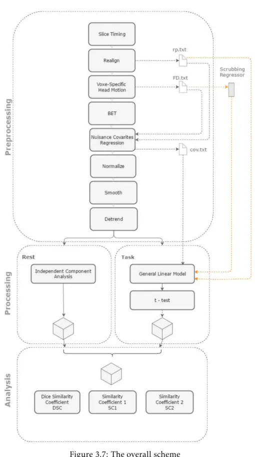
This chapter is intended to explain how the current study was conducted, undergoing a brief exposition of the software and methodology implemented. The chapter begins with a description of the subjects who participated in the study as well as the parameters of image acquisition. Then, detailed information about the methods and software used in the pre-processing of the acquired data is reported, followed by the explanation of the strategies used to process the images and to extract the activation networks of task and rest paradigms. Finally, it is explained how the neural maps were superimposed and its correlation calculation.
3.1 Participants and Image acquisition
This research gathered data provided by Hospital Cruz Vermelha. A total of 8 partici-pants were recruited to participate in this study. All of them were previously referred for surgical resection of a brain lesion. The demographic characteristics of the participants are reported in table 3.1.
All patients were scanned using a 3-T (Philips Achieva by Philips Medical System, Netherlands). A gradient echo sequence was applied and the first three volumes were discarded in order to achieve a homogeneous magnetization. The data acquisition protocol consists of the following steps.
Table 3.1: Demographic features of the study population
Subject ID Sex Age
Sub001 M 19
Sub002 M 26
Sub003 M 37
Sub004 M 33
Sub005 M 14
Sub006 M 31
Sub007 M 32
Sub008 F 35
(TE)=4.6ms.
Functional images were acquired with a matrix of 128x128 and a flip angle of 90◦. For the rs-fMRI acquisition the patient is requested to stare at a black screen, without closing his eyes or making any other ocular movement. The scanning lasts 5 minutes, cor-responding to 150 volumes of the entire brain. The voxel size was 2x2x3mm3,TR=2000 ms and TE=23 ms.
For the task paradigm the subjects had to perform blocks of tasks prompted by a stimulus. The stimuli were displayed visually and required the ability to read. Language tasks include detection of semantic and syntactic errors as well as sentence processing.
Language tasks paradigms consist of:
• Semantical Decision: detection of equals (=) or number signs (#) in the displayed sentences. The sentences were presented according to 3 different frequencies (low,
medium, high), composed by two blocks each. Paradigm begins and ends with a rest block.
• Synctatic Decision: 3 tested tasks: gender concordance, temporal conjugation and the correct use of pronouns, each composed of two interleaved blocks. Paradigm begins and ends with a rest block.
• Verb Generation: 4 blocks of linguistic stimuli interspersed with 4 blocks of visual but not linguistic stimui, such as circles and number signs.
was 2x2x4 TR was 2000ms and the TE was 23 ms . In respect of motor tasks, these consist of:
• Mouth: 4 task blocks (opening and closing), interspersed with 4 rest blocks. The paradigm begins with the completion of the task.
• Hand: 4 task blocks of hand bilateral motion, interspersed with 4 rest blocks. The paradigm begins with the completion of the task.
• Feet: 4 task blocks of feet bilateral motion, interspersed with 4 rest blocks. The paradigm begins with the completion of the task.
Task acquisitions comprises 80 holocranial volumes, a voxel size of 2x2x4, TR=3000 ms and TE= 33 ms.
3.2 Preprocessing
Data pre-processing was accomplished using a MATLAB® (The MathWorks Inc., MA, USA version R2013a) implemented toolbox called Data Processing Assistant for Resting-State fMRI- advanced edition (DPARSFA) (Chao-Gan and Yu-Feng, 2010). DPARSFA is an user-friendly tool whithin Data Processing and Analysis for Brain Imaging (DPABI) and it is based on some functions in Statistical Parametric Mapping (SPM) (developed by members and collaborator of The Wellcome Trust Centre for Neuroimaging Institute of Neurology, University College London) and Resting-State fMRI Data Analysis Toolkit (REST) (Xiao-Wei Song, 2011). DPARSFA accepts structural and functional data in Dig-ital Imaging and Communications in Medicine (DICOM) format, which is an universal output format of fMRI scans.
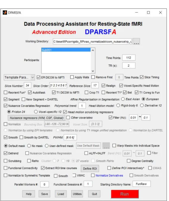
The main purpose of this part of the study was essentially to choose the combination of pre-processing parameters that best suited the ultimate goal, which was to recognize and extract task and rest networks. The software template is displayed in fig 3.1.
The pre-processing was performed individually for each subject and one paradigm at a time. Task data and rest data were pre-processed following different pipelines.
Below is described pre-processing steps on both cases.
• DICOM to Neuroimaging Informatics Technology Initiative (NIfTI)
The first step was to convert DICOM files to NIfTI format. This format includes the affine coordinate system, which transforms voxel index (i,j,k) to spatial
right hemisphere is. In DPARSFA functional and structural data are converted independently.
• Remove first time points In the scope of this study, it wasn’t required to discard the first volumes since this has already been done as part of the standard acquisi-tion procedure.
• Slice timing This option was checked with the purpose of correcting differences
in image acquisition time between slices.
Slice Number The slice number consists of 38 axial slices acquired contin-uously for motion paradigms. In semantic, syntactic, verb generation and rest paradigms the number of slices is 34.
Slice order Slices were acquired one by one from anterior to posterior, from left to right and from bottom to top. Therefore, this option was filled with an array going from 1 to number of slices.
Reference slice The reference slice was set to the slice acquired at halfway the scan in order to reduce timing corrections.
• Realign - The realignment is applied by rigid body transformations, which as-sumes that the shape and size of the volumes are the same and that one image can be spatially matched to the first image, which SPM set it as reference, by the com-bination of three translation (x,y,z; in mm) and three rotation parameters (pitch, roll, yaw; in degrees). These operations are performed by matrices and can then be multiplied together. See equation 3.1. Furthermore, one .txt file is created with each volume’s motion specified for each axes and can be further applied as part of nuisance regressor.
1 0 0 Xt
0 1 0 Yt
0 0 1 Zt
0 0 0 1
×
1 0 0 0
0 cosΦ sinΦ 0
0 −sinΦ cosΦ 0
0 0 0 1
×
cosΘ 0 sinΘ 0
0 1 0 0
−sinΘ 0 cosΘ 0
0 0 0 1
×
cosΩ sinΩ 0 0
−sinΩ cosΩ 0 0
0 0 1 0
0 0 0 1
(3.1)
Its goal is to minimize the difference of head motion impact on the voxels,
depend-ing on their distance from the center of the gradient coil. One text file is created and comprises frame-wise displacements (FD) from the reference image for each volume. This file is further applied in the scrubbing regressor calculation.
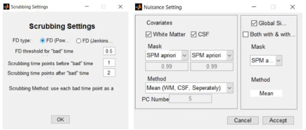
• Nuisance Covariates Regression Nuisance signals are those originating from non-neural sources and can cause spurious activations.
Nuisance regressors Respiration and the cardiac signal are among the sources of those artifactual signals. As these physiological sources are not recorded along with the fMRI scan, it is possible to remove them based upon their frequency. For this purpose nuisance covariates may include global mean signal (respiratory and cardiac cycle), cerebrospinal fluid (CSF) and white matter (WM) signal, figure 3.2. In this study all the covariates mentioned above were regressed out by GLM.
Head Motion Model In addition to physiological signal regressors, motion regressors were added to GLM model. Those motion regressors included the 6 head motion parameters estimated in the realigment option, plus 6 head motion parameters one time point before, and the 12 corresponding squared items, that are all comprised in Friston 24-parameter model, (Friston et al., 1996 [34]).
Head motion scrubbing regressors As a final step, head motion scrubbing regressors were generated to be further included in the model. The scrubbing method identifies motion-induced spikes and rejects them based upon a defined FD threshold. Of note that FD were previously estimated on voxel-specific head motion option. In this study, the FD threshold for "bad" time point was 0.5 mm, i.e. all the time points that were displaced 0.5 mm from the first time point considered corrupted. According to the guidelines of Power et al. (2012b), the bad time points as well as 1 before and 2 after neighbours were also excluded from data, figure 3.2. DPARSFA produces one regressor for each time point excluded.
In conclusion, nuisance covariates removes physiological, non-neuronal noises from data, and produces a matrix of regressors (or covariates) where each line characterizes one time-point, and each column represents 24 motion parameters, plus WM, CSF and global mean signal, and an undefined number of scrubbing regressors.
results and its application or not as preprocessing stage was analyzed.
a Scrubbing Settings b Nuisance Settings
Figure 3.2: DPARSFA options
• brain extraction tool (BET) BET was used to remove non-brain areas.
• Normalize The acquisition of fMRI images may vary depending on the intended purpose. Thus the position, angle and dimensions of the images obtained are specific for each paradigm. So that images become comparable it is essential that all of them are normalized to the same space. Normalize function is used to put scans into Monreal Neurological Institute (MNI) space. This function understates the differences between two scans by minimizing the sum of squares of intensity
differences. The normalization can be based on the standard template (MNI),
however in subject-specific studies, as the present study, it is preferable to use the patient’s anatomical images as a template. Voxel size that best fits the data of this study was [3 3 3] and bounding box’s measures were specified by SPM itself. Normalize option requires co-registration and segmentation.
Segment Segment separates grey matter, white matter, and CSF in anatomical images.
Structural Coregistration to Functional Coresgistration aligns functional im-ages into the same space and orientation of anatomical ones. Besides, any trans-formations in structural data can be applied in functional images.
as make the data more complying with the specifications of the underlying sta-tistical theory (Gaussian Random Fields). This was accomplished by convolving the images with a Gaussian kernel. In order to achieve the best pre-processing pipeline, several kernel sizes were tested. From the matched filter theorem, the best kernel size is about the same size as data activation. As it wasn’t known, at the pre-processing stage, the precise size of activations, although it was known that they wouldn’t be much significant, the size of the Gaussian that best suited the study’s interest was a small one with full width at half maximum (FWHM) of 6 mm, which is in concordance with previous studies and follows a well-established rule of thumb that suggests that the kernel width should be about 2 to 3 times voxel size.
• Filter Temporal filtering was performed by a 0.01- 0.1 Hz bandpass filter, remov-ing low-frequency drifts and physiological high-frequency respiratory and cardiac signals.
• Detrend Several studies demonstrated the importance of removing linear trends in voxel time courses in individual subjects. The origin of these trends is not com-pletely understood, but they occur due to long-term physiological shifts. DPARSFA relies on REST to estimate the linear trends with a least-square fitting of a straight line, which is removed from the data. Subsequently, the original mean value of each time course is added back.
• Scrubbing To save computational time, scrubbing option was not performed in pre-processing stage, since it was previously included as a regressor on nuisance matrix.
3.3 Processing
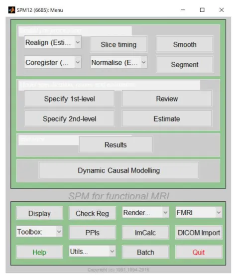
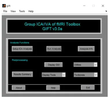
Task data was processed whith SPM, while rest data was processed with Group ICA of fMRI toolbox (GIFT).
3.3.1 Task data - Statistical Analysis
Figure 3.3: SPM layout
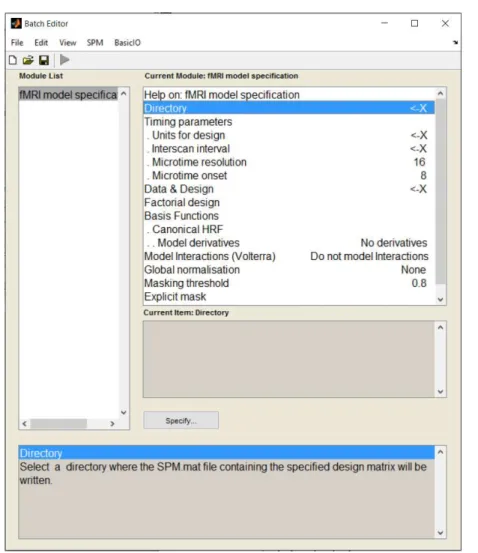
3.3.1.1 Model specification
GLM identifies the areas with significant BOLD signal change, induced by cognitive tasks. For that purpose the signal model was constructed by convolution of canonical hemodynamic response function (hrf) with the boxcar function of each task, including the pre-processing nuisance regressors. Both hrf and model regressors were designed based on scan numbers, i.e., the first scan corresponds to timepoint zero and the second one corresponds to timepoint 1, and so on. The time between the start of sequential scans, or interscan interval, was established based upon TR (2s for linguistic paradigms and 3s for motion paradigms).
Figure 3.4: fMRI model specification
paradigm for one subject. In the context of feet, hands, mouth and verb generation paradigms, only one boxcar condition was defined per session, since those cases re-flected on-offstimulation paradigms. On the other hand, 4 conditions were setted for
each semantic and syntactic task. As regards to semantic decision, the 4 conditions describe the 3 frequencies of the stimuli (low, medium, high) and the free-stimulus condition at the beginning and end of the task. Relatively to syntactic decision, the 4 conditions were gender concordance, temporal conjugation an correct use of pronouns, including the free-stimulus condition at the beginning and end of the task. The onset times and the period of the stimulation were specified in the SPM framework.
or not. In the first case, a multiple regression was performed resorting to nuisance covariates matrix created in the pre-processing stage. On the other hand, head motion regressors were included in the model through realignment parameters’ text file and an additional regressor in cases where the subject performed to much movement. The latter array was created using MATLAB® functions and attempted to reproduce head motion scrubbing regressor. For this purpose, the construction of the array resorted on the framewise displacement of each volume. If the displacement was higher than 0.5 mm then that volume, such as the one before and the two after adjacent volumes were excluded, ie were represent by an ‘0’ in the vector. The remaining volumes acquire the value ‘1’.
Masking data aims to only estimate voxels that seem to have significant signal in them. As for the default SPM sets masking threshold threshold to 0.8, which means that the model is estimated based on voxels whose mean value is at 80% of the global signal. However if nuisance covariates regression formed an integral part of the pre-processing, this threshold has to be setted to -inf. As the significance of the activation voxels is low, mask that include all brain, and not a specific portion, was applied.
3.3.1.2 βestimation and contrast
After the model be established, GLM estimatedβvalues using an autoregressive model during restricted maximum likelihood (ReML) parameter estimation, which assumes that each voxel has the same error correlation structure.
Onceβwere estimated, we tested if the most significantβwere assigned to the most important regressors of the model, in other words, if the most important regressor was greater than 0. Within the context of this experiment, the most important regressors were the ones that describe the defined conditions. To test that, we relied on GLM T-contrasts to define the hypothesis and t-test to assess it.
In GLM, a contrast specifies linear combinations ofβ. In motion paradigms context, as only one on-offcondition was defined for each motion, a simple contrast was applied.
h
1 0 0 ··· 0ni
Where n is the number of regressors.
In the case of semantic and syntactic paradigms, a weighted contrast between the different conditions, plus a -1 weighted, to ensure that the sum of weights was zero, was
h
0 13 13 13 −1 0 ··· 0ni
Finally in verb generation, where the model responses to two conditions (verb gen-eration + baseline), a [1,-1] contrast was established to compare the two conditions. Hence, the secondβ was subtracted to the first before it was tested against zero, i.e,
β1−β2>0 .
After definingt-contrasts, SPM performed at-test, which estimatedtvalues for the whole brain by calculating the ratio of the contrast of the estimated paradigms by the deviation of variance, equation 3.2.
t=contrast of estimated parameters√ variance estimate ⇔t=
c′β
p
s2c′(X′X)c (3.2)
At last, severalp-thresholds (corrected and uncorrected) were assessed for each task of each participant, in order to maximize the number of true positives while reducing the false ones.
3.3.2 Rest data processing
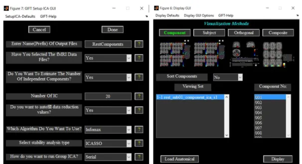
Figure 3.5: GIFT layout
Just like the studies mentioned above, components were estimated for each subject using the minimum description length (MDL) criteria. ICA maps were generated for 20 and 50 independent components using Infomax algorithm. In order to determine the reliance and stability of the previously selected ICA algorithm, ICASSO toolbox was applied. ICA algorithm ran 5 times, and each run started with a different initial value
(RandInit), figure 3.6.
The extracted independent components were then visually assessed using the soft-ware display option, figure 3.6
.
3.4 Comparison of Task Networks and Resting State Networks
In order to evaluate how rest activation maps are related to task activation maps, diff
er-ent similarity coefficients were employed. The precedent procedures that characterize
this analysis are described below.
For each task of each participant, 4 different activation maps were created in SPM.
a ICA model specification b GIFT display GUI
Figure 3.6: GIFT options
• FWE 0.05;
• FWE 0.01;
• FWE 0.1;
• Uncorrected 0.001.
Activation maps for task paradigms were then binarized using an option provided by SPM, allow to obtain a 3D image in nifti format, where 1 represents the significant activations for the selected p-value. The binarization step is essential to implement the similarity coefficients, as will be explained later in this section.
In the meantime, binarization of the rest activation maps was achieved by using 9 intensity thresholds, applied to each independent component previously extracted in the GIFT software. These thresholds varied between 10% and 90% of the total’s intensity, with an increment of 10% between each.
The resemblance between the binarized images was subsequently calculated with 3 different coefficients. The first one, which is one of the most used, is the Dice similarity
DSC = 2|R∩T|
|R|+|T| (3.3)
The numerator is the overlap between the activations of rest (R) and task (T) bina-rized maps, and the denominator is the sum of both.
This coefficient takes values between 0 and 1, wherein 1 is the perfect overlap,
whereas 0 describes the opposite event. A low value of the DSC can represent one of two situations: the intersection of rest and task activations is low or the union between the two activations is high. As the reason why Dice coefficient might be low can not be
directly measured by this index it became necessary to create two more indexes. One of them, equation 3.4, is a measure of the overlap of rest activation maps on task activation maps, ie, if the index has the value 1, means that all task activations match rest activations, however does not directly imply that all the rest activations coincide with task activations. This coefficient, will be henceforth designated by Similarity Coefficient
1 (or SC1).
SC1=|
R∩T|
|T| (3.4)
Lastly, equation 3.5 attempts to find the contribution of rest activations in the over-lap of the two maps. This coefficient, will be hereinafter designated by Similarity
Coef-ficient 2 (or SC2). If this index is close to 1 it means that there are no coincidences on where the rest and task activations take place.
SC2=
R∩T
|R| (3.5)
C
h
a
p
t
4
R e s u lt s
This chapter is intended to report the most relevant results obtained in pre-processing and processing stages, followed by the presentation of statistical and similarity analysis results. Due to the large volume of data, results from the latter will be presented in two different approaches. One intends to present the outcomes of all tasks for a single
participant, and the other approach aims to present the results of one single task for all subjects. The selection criterion of the subject and task to present in this section is the minimum number of volume removed by the scrubbing procedure.
4.1 Important results from preprocessing
As the design of a preprocessing protocol was a key part of this research, herein are the results of some of the parameters which arouse more questions.
4.1.1 Scrubbing
From the information presented in the table, it is possible to affirm that subject
003 is the one with fewer volumes removed, alongside with Sub006. For the first one, only hands motor paradigm led to a framewise displacement greater than the value stipulated by Power et al., while in the second one volumes were withdrawn only in the syntactic decision. Subject 005 is the one with the largest number of volumes removed, since in all tasks, and rest included, several volumes had to be regressed out. Another finding worth mentioning is the major impact of scrubbing on language paradigms for subject 001 and 002, since only 10 time points remain in each paradigm.
Regarding to tasks, the feet paradigms are noted for producing the largest number of removals between the motor tasks, while the semantic decision stands out among the linguistics. In rest, few or none volumes were removed, excepting for Sub005.
Table 4.1: Scrubbing Results
Subject ID
Motor Paradigms Linguistic Paradigms
Rest
Mouth Hands Feet Semantic Decision
Syntactic Decision
Verb Generation
Sub001 0 10 0 150 150 150 0
Sub002 4 0 34 150 150 150 4
Sub003 0 4 0 0 0 0 0
Sub004 14 0 0 0 0 0 0
Sub005 55 51 62 150 85 30 56
Sub006 0 0 0 0 13 0 4
Sub007 0 0 12 0 4 0 4
Sub008 0 4 0 36 9 27 4
4.1.2 Normalization
As mentioned in section 3.2, the image acquisition is different for motor tasks and for
rest and language tasks. This difference is more evident in the images dimensions.
The dimensions of motor tasks images are 128x128x38 while rest and language tasks images have a dimension of 128x128x34, which results in an inconsistent comparison and in the impracticability of similarity analysis between the motor tasks data and rest. To illustrate this difference, the figure 4.1 contains a representation of mouth task
a Mouth task, immediately before normalization b Semantic Decision, immediately before nor-malization
c Mouth task, immediately after normalization d Semantic Decision, immediately after normal-ization
Figure 4.1: Difference between normalize and not normalize images. The upper images
4.1.3 Removal of nuisance signals
The removal of the nuisance signals includes removing all non-neuronal signals and pro-duces the visual effect illustrated in fig 4.2. The sub figure related to the performance
of this procedure is much more blurred than one that not contemplates it.
Despite the removal of nuisance signals produce an overly blur effect it is not
auto-matically indicative of a worse activations extraction. Thus, to test the efficiency of this
procedure two analysis were carried out in parallel, one using this procedure and the other not. The results of these two analysis are available in section 4.2.1.1.
a Mouth task, immediately before removing nui-sance signal
b Mouth task, immediately after removing nui-sance signal
Figure 4.2: Effect of nuisance signals removal. These images belong to the subject under
4.2 Intra-Subject Analysis
This section aims to present the results in an intra-subject perspective. Thus, the results of activations mapping of all task paradigms and at rest will be presented for subject 003. The choice of this subject, as mentioned earlier in this chapter, is related to the small number of volumes removed by scrubbing (consult table 4.1).
4.2.1 Motor Paradigms
4.2.1.1 Mouth paradigms
As described in section 3.4, similarity tests were conducted by resorting to 4 distinct maps coming from Statistical Parametric Mapping SPM. Each map results from a diff
er-ent significance level. The visual effect of selecting differentp-values can be found in
![Table 2.1: Brain tumor classification [12] [13] [14]](https://thumb-eu.123doks.com/thumbv2/123dok_br/16548153.737032/26.892.164.789.178.720/table-brain-tumor-classification.webp)
![Figure 2.1: Classic anatomic sites for functional brain areas [41].](https://thumb-eu.123doks.com/thumbv2/123dok_br/16548153.737032/33.892.179.664.630.1005/figure-classic-anatomic-sites-functional-brain-areas.webp)
![Figure 2.2: Resting-State networks [38]](https://thumb-eu.123doks.com/thumbv2/123dok_br/16548153.737032/34.892.199.748.153.781/figure-resting-state-networks.webp)