Towards improving WEBSOM with Multi-Word Expressions

(1)

Stefan Eduard Raposo Alves

No35098

Towards improving WEBSOM with Multi-Word

Expressions

Dissertação para obtenção do Grau de Mestre em Engenharia Informática

Orientador : Nuno Cavalheiro Marques, Prof. Doutor, Universidade Nova de Lisboa

Co-orientador : Joaquim Ferreira da Silva, Prof. Doutor, Universidade Nova de Lisboa

Júri:

Presidente: Henrique João Arguente: Carlos Ramisch

(2)

(3)

iii

Towards improving WEBSOM with Multi-Word Expressions

Copyright cStefan Eduard Raposo Alves, Faculdade de Ciências e Tecnologia,

Univer-sidade Nova de Lisboa

(4)

(5)

(6)

(7)

Abstract

Large quantities of free-text documents are usually rich in information and covers several topics. However, since their dimension is very large, searching and filtering data is an exhaustive task. A large text collection covers a set of topics where each topic is affiliated to a group of documents. This thesis presents a method for building a document map about the core contents covered in the collection.

WEBSOM is an approach that combinesdocument encodingmethods and Self-Organising

Maps (SOM) to generate a document map. However, this methodology has a weakness in the document encoding method because it uses single words to characterise docu-ments. Single words tend to be ambiguous and semantically vague, so some documents can be incorrectly related. This thesis proposes a new document encoding method to improve the WEBSOM approach by using multi word expressions (MWEs) to describe documents. Previous research and ongoing experiments encourage us to use MWEs to characterise documents because these are semantically more accurate than single words and more descriptive.

(8)

(9)

Resumo

Uma enorme quantidade de documentos de texto é geralmente rica em informações e abrange diversos tópicos. No entanto, uma vez que a sua dimensão é muito volumosa, a pesquisa e filtragem de dados torna-se numa tarefa exaustiva. Um coleção grande de textos aborda um conjunto de temas onde cada tema é associado a um grupo de docu-mentos. Esta tese apresenta um método para gerar um mapa de documentos sobre os principais conteúdos abordados numa coleção volumosa de textos.

A abordagem WEBSOM combina métodos de codificação de textos com Mapas Auto-Organizados (Self-Organising Maps) para gerar um mapa de documentos. Esta metodo-logia tem uma fraqueza na codificação de textos, pois utiliza apenas palavras singulares como atributos para caracterizar os documentos. As palavras singulares têm têndencia para ser ambíguas e semanticamente vagas e por isso alguns documentos são incorre-tamente relacionados. Esta dissertação propõe um método para codificar documentos através de atributos compostos por expressões relevantes. Através de estudos efetuados verificou-se que as expressões relevantes são bons atributos para caracterizar documen-tos, por serem semanticamente mais precisas e descritivas do que palavras singulares.

Palavras-chave: Self-Organising Maps (SOM), Text Mining , WEBSOM, Expressões

(10)

(11)

List of Figures

1.1 Example of the system interaction with WEBSOM. . . 2

2.1 An agglomerative clustering using thesingle-linkmethod.. . . 7

2.2 K-means clustering result for the Iris flower data set and the real species distribution usingELKI. . . 8

2.3 Example of an input vector update when fed to the network. . . 12

2.4 U-matrix and respective labelling using the iris data set.. . . 13

2.5 Component Planes for the Iris data set.. . . 13

2.6 A map of colours based on their RGB values. . . 14

2.7 The original WEBSOM architecture. . . 19

2.8 Case study in [1]: A Usenet Newsgroup. . . 20

2.9 Case study in [2]. . . 22

2.10 Case study in [3]. . . 24

3.1 Proposed Architecture. . . 27

3.2 Reduction example. . . 29

3.3 Example of the differences between applying the simple probability and the probability weighted by itself.. . . 31

3.4 Example of the differences between applying the simple probability and the probability weighted by UMin . . . 32

3.5 Reduction example. . . 34

3.6 A smallneural networkwith petrol news. . . 37

3.7 Example of MWE "light sweet" component plane. . . 39

3.8 Example of MWE "nova iorque" component plane. . . 40

4.1 Plots for quantisation and topographic errors- . . . 48

4.2 Document map for the abstracts collection. . . 51

4.3 Document map for the News collection. . . 53

(14)

xiv LIST OF FIGURES

(15)

List of Tables

2.1 Some common measures used in hierarchical clustering. . . 6

2.2 models . . . 9

3.1 Top MWEs between documents 3 and 5 havingwk,i=pk,i. . . 33

3.2 Top MWEs between documents 3 and 5 havingwk,i=UM ink,i. . . 33

3.3 Top MWEs between documents 3 and 5 havingwk,i=UInvk,i. . . 35

3.4 Top MWEs for neurone 31. . . 37

3.5 Top MWEs for neurone 32 . . . 38

4.1 Types of documents . . . 41

4.2 Collection using the U metric . . . 43

4.3 Collection using the UMin metric . . . 43

4.4 Probability values in respective document. . . 44

4.5 Multi-Word Expressions scores. . . 44

4.6 Collection using the Invert Frequency Metric . . . 44

4.7 Sample connector . . . 45

4.8 Sample correlation . . . 46

4.9 Sample correlation . . . 46

4.10 Abstracts results . . . 48

4.11 Training Duration. . . 48

4.12 Quantisation and Topographic Errors for the Abstract collection.. . . 49

4.13 Field Purity and Empty Rate for the Abstract collection. . . 49

4.14 Precision and Recall for the Abstract collection. . . 50

4.15 Samples of Abstract neurones . . . 52

4.16 Samples of News neurones. . . 55

(16)

(17)

1

Introduction

1.1 Motivation

Large quantities of free-text documents can be seen as a large disorganised encyclopae-dia. This text collection is rich in information but searching and filtering data is an ex-haustive task. A large text collection covers a set of topics where each topic is affiliated to a group of documents. A document map about the core contents covered in the col-lection can be build by identifying the topics addressed in the documents. This is the main motivation for this thesis that aims to develop a document map that can relate doc-uments not only by expressions in common but also with semantic associations. These associations occur when documents share the same topic but use different terms in their description, however, by identifying common patterns in documents, it is possible to re-late them. Furthermore, a semantic map combined with a search engine responds faster in locating specific documents in answer to information requests, because the map has the documents organised and compressed by topics.

The emerging field of text mining applies methods to convey the information to the user in an intuitive manner. The methods applied vary according to the type of docu-ments being analysed and the results that are intended. In this study, the different types of documents used are known as snippets, that are: parts of news, parts of reports and

abstracts of articles. We intend to compose acorpus with these types of text and then

build a context map about the core contents addressed in these documents.

The starting motivation for this dissertation was the need of building Corporate

Se-mantic Maps in the context of the parallel ongoing project BestSupplier1. Best Supplier

1

(18)

1. INTRODUCTION 1.1. Motivation

project needs to extract textual information related to companies. In the project frame-work, Self-organising maps were soon considered as a valuable tool for retrieving

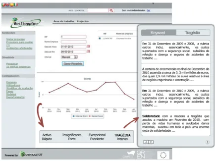
rela-tions among documents and their summarisation. Figure1.1presents the initial

informa-tion retrieval concept (as shown in [4]), that aimed to use snippets extracted form

com-pany reports (exemplified on the right of the figure) for mining related information and for building a Corporate Semantic Map. Latter, the Corporate Semantic Map could be used to relate concepts with documents. However, sharp semantic features were needed and the original WEBSOM soon showed its problems regarding a straight forward ap-proach. This way, since the field studied by this project revealed to be too large to be analysed in this dissertation, a more academic perspective was chosen that yet, was still beneficial for the global project: trying to study how to improve WEBSOM quality by using better semantic aware features. The WEBSOM methodology has a weakness in thedocument encoding method because this one uses single words to characterise docu-ments. Single words tend to be ambiguous and semantically vague, so some documents can be incorrectly related. This tends to be semantically less accurate than a well formed multi-word expressions.For example, the word "coordinates" is ambiguous because it has

more than one meaning: brings into proper place or order/a set of numbers used to calculate

a position. However, if "coordinates" it is taken within a relevant expression (RE), such as "map coordinates" or "coordinates the project", there is no ambiguity since it gains se-mantic sharpness. The fragility related to the poor accurate features used in the original WEBSOM builds up an important motivation of this thesis.

,QVLJQLILFDQWH )RUWH ([FHSFLRQDO([FHOHQWH $FWLYR

5iSLGR

(PGH'H]HPEURGHHDUXEULFD RXWURV LQFOXL HVVHQFLDOPHQWH RV FXVWRV VXSRUWDGRVFRPDVHJXUDQoDVRFLDOVXEVtGLRVGH UHIHLomR H GRHQoD H VHJXURV GH DFLGHQWHV GH WUDEDOKR

$

$FDUWHLUDGHHQFRPHQGDVQRILQDOGH'H]HPEURGH DVFHQGLDDFHUFDGHPLOPLOK}HVGHHXURV GRVTXDLVPLOPLOK}HVGHHXURVUHODWLYRVjiUHD GHQHJyFLRHQJHQKDULDHFRQVWUXomR

(P

(PGH'H]HPEURGHHDUXEULFD RXWURV LQFOXL HVVHQFLDOPHQWH RV FXVWRV VXSRUWDGRVFRPDVHJXUDQoDVRFLDOVXEVtGLRVGH UHIHLomR H GRHQoD H VHJXURV GH DFLGHQWHV GH WUDEDOKR

6ROLGDULHGDGH

6ROLGDULHGDGH FRP D PDGHLUD D WUDJpGLD TXH DVVRORX D PDGHLUD HP )HYHUHLUR GH FRP SHUGD GH YLGDV KXPDQDV H DYXOWDGRV GDQRV PDWHULDLVVXVFLWRXHPWRGRRSDtVXPDHQRUPH RQGDGHVROLGDULHGDGH

.H\ZRUG

(19)

1. INTRODUCTION 1.2. Objectives

1.2 Objectives

The main focus of this thesis is to develop a document map about topics addressed in documents, using self-organising maps. The WEBSOM addresses this field applying text-mining methods, however, this approach uses single words to characterise documents. Our goal is to extend the WEBSOM module in a manner that documents are characterised by relevant expressions (REs), because these are semantically more accurate than single words. The following requirements are the goals that are intended to accomplish:

Goal 1. Extract the snippets content by their REs:

Snippets are composed by textual data with some dimension. This text size can be compressed into a set of REs that describe the main content of it. So, we in-tend to learn how to extract all possible meaningful expressions that describe the documents core content.

Goal 2. Measure and weight REs:

As it was said before, the content of a snippet is compressed in a set of REs. Al-though the description of the snippet is obtained according to that set, there are expressions that are more informative than others. In this goal a measure to weight

the relevance of each RE in the corpusis developed. By measuring the terms

ex-tracted ingoal 1, it is possible to determine which are those that are more influential

in the collection. For instance, an expression may be a relevant and well composed multi-word, but if it occurs very often in the majority of documents, it is not very

influential. Besides, since the extractor used ingoal 1also extracts some incorrect

REs, not all of them are well formed multi-word expressions and it is necessary to penalise these ones.

Goal 3. Reducing the document features dimension:

The documents in text-mining are usually represented as a vector of the size of the vocabulary where each position corresponds to some function of the frequency of a particular keyword in the document. For this study, keywords are REs extracted ingoal 1, which results in a vast dimensionality of the document vectors because

the number of REs in acorpuseasily rises to tens of thousands. Typically, a huge

number of features is computationally heavy for clustering algorithms, besides, the results may lose precision. So, in order to reduce the number of features, this study

proposes to represent documents in adocument-by-documentvector where each

doc-ument is characterised by its similarities with all the other docdoc-uments. Similarities are calculated considering all REs in the vocabulary.

Goal 4. Develop a semantic map using WEBSOM:

(20)

1. INTRODUCTION 1.3. Structure of the thesis

organise a textual collection onto a two-dimensional projection designated as con-text map. In order to extend the WEBSOM module with REs it is necessary to

com-bine the structure produced ingoal 3with the SOM. So, this dissertation intends to

study the WEBSOM module to build a document map from the structure produced in the previous goal.

Goal 5. Combine the semantic map with REs:

The semantic map reflects an organised collection of documents, where documents with similar attributes are close in the map and dissimilar documents are in differ-ent areas. Although this structure is useful, it is necessary to understand why the documents are together in a intuitive manner. Since the map has similar documents placed in the same area, it is possible to determine the main REs responsible for that document proximity in the map, and then represent these locations with them. So, as meaningful REs give a strong perception of the main core content of documents, a method is proposed to visualise the impact of REs in the semantic map.

1.3 Structure of the thesis

Chapter 2 is the result of a literature study that forms the basis of this thesis. A brief

overview about clustering algorithms and their application to document clustering is

done. Then, the WEBSOM method and keyword extractor is presented. Chapter3

pro-poses an approach, designated as RSOM, for the document clustering method in the con-text of document Information Retrieval techniques. This chapter also outlines the

archi-tecture chosen for this approach. Chapter4evaluates and exemplifies the application of

(21)

2

Related Work

In this Chapter a study about different types of text-mining algorithms to conduct this

dissertation is presented. First, Section2.1performs an analysis about existing clustering

methodologies. Then, Section2.2presents an approach to represent specific data such as

free-text for document clustering algorithms. Section2.3describes the WEBSOM module

and identifies the components which have to be modified to integrate REs. Moreover, why the REs can be a solution to solve the semantic fragility of individual words is also

discussed. The following Section2.4presents a detailed description about a REs extractor

used in this study.

2.1 Clustering

2.1.1 Hierarchical clustering

Hierarchical clustering [5] is a data-mining algorithm which aims to cluster objects in

such a manner that in a cluster objects are more similar to each other than instances in different clusters. As the name suggests, clusters are formed hierarchically according to a "bottom up" or "top down" approach. In other words, there are two ways to form hierarchical cluster:

• Agglomerative clusteringis a "bottom up" approach which begins with a cluster for each training object, merging pairs of similar clusters as it moves into higher levels of the hierarchy, until there is just one cluster.

(22)

2. RELATEDWORK 2.1. Clustering

one cluster for each training object.

Both agglomerative and divisive clustering determine the clustering in a greedy

al-gorithm1. However, the complexity for divisive is worse than agglomerative clustering,

which isO(2n₎_and_O₍_n3₎_{respectively, where}_n_{is the number of training objects.}

Fur-thermore, in some cases of agglomerative methods a better complexity ofO(n2)has been

accomplished, namely:single-link[6] andcomplete-link[7] clustering.

Measure Name Measure Formula

Euclidian distance d(x, y) =pP2

i(xi−yi)2

Manhattan distance d(x, y) =P

i|xi−yi|

Maximum distance d(x, y) = max

i |xi−yi|

Cosine similarity d(x, y) = _k_xx_kk·y_y_k

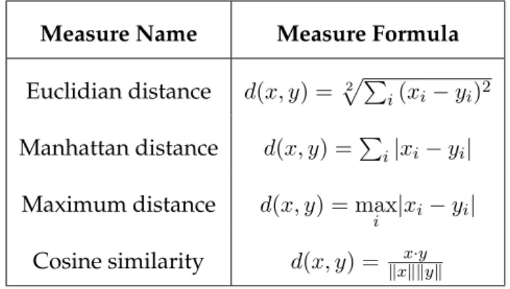
Table 2.1: Some common measures used in hierarchical clustering.

In single-link clustering, the distance is defined as the smallest distance between all possible pair of objects of the two clusters:

d(Cx,Cy) = min

x∈Cx,y∈Cy d(x, y)

whered(x, y)is a generic distance measure between objectxandy. Some common

mea-sures used in hierarchical clustering are displayed in table2.1. Incomplete-link clustering,

the distance between two clusters is taken as the largest distance between all possible clusters:

d(Cx,Cy) = max

x∈Cx,y∈Cy

d(x, y).

The previous methods are most frequently used to choose the two closest groups to

merger. There are other methods such as theaverage-linkmethod that uses the average of

distances between all pairs and the centroid2distance between two clusters.

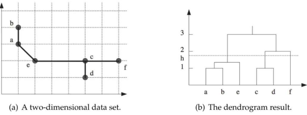
The result obtained using a hierarchical clustering algorithm is generally expressed as adendrogram. An example is given in figure2.1with thesingle-linkmethod, where the

lower row in figure2.1(b)represents all instances, and as we go into higher levels,

clus-ters are merged according to their similarities. Thehvalue represents the hierarchy level

that determines the number of clusters, which is the minimal number of clusters having

all objects with distance lower than h. Althoughcomplete-linkforms clusters differently

1

A greedy algorithm is an algorithm that solves the problems according to a heuristic to make the local optimal choice at each stage.

(23)

(a) A two-dimensional data set. (b) The dendrogram result.

Figure 2.1: An agglomerative clustering using thesingle-linkmethod.

fromsingle-link, the number of clusters is determined in the same manner. In general,

this requirement occurs in both agglomerative and divisive clustering. The value ofh

is specified by the user, which makes this algorithm inadequate for aim of this disserta-tion because the number of clusters should be formed according to object attributes in a

natural way.

2.1.2 K-means and k-medoids

K-means [8] is a data-mining algorithm which aims to distribute data objects in a defined

number ofkcluster where each object belongs to the cluster with nearest centroid. This

clustering results in a partition of the data space intoVaronoi diagrams[9]. In other words

for a datasetX= (x1, x2, ..., xn)in whichxi is ad-dimensional real vector,k-means aims

to partition thenobjects into kclusters C = (c1, c2, ..., ck) so as to minimise the within

cluster sum of squares:

arg

C

min

k

X

i=1

X

xj∈X

kxj−µik2

whereµiis the centroid of clusteri.

An inconvenience of k-means lies on the fact that the objects distance is measured

by the Euclidean distance because it is assumed that the clusters are spheroids with the same size, which does not occur in most real cases. In fact, in most clustering configura-tions, each cluster presents its own volume, shape and orientation. An example of this

behaviour can be visualised in figure2.2 that is a k-means clustering result for theIris

flower data set3[10] and the real species distribution using theELKI4framework, in which the cluster centroid is marked using a larger symbol.

K-medoids clustering [11] is a partitioning algorithm similar to k-means algorithm.

In contrast, instead of building centroids, this one chooses objects from the data set as cluster centres (medoids or exemplars). This method is more robust to noise and

out-liers in comparison tok-means because it minimises the sum of pairwise dissimilarities

3

The Iris flower dataset is a data collection about variation of Iris flowers of three related species.

4

(24)

Figure 2.2: K-means clustering result for theIris flower data setand the real species

distri-bution usingELKI.

instead of the sum of squared Euclidean distances.

The number of clusters has to be specified in bothk-means andk-medoids. This

re-quirement makes these algorithms inadequate for a fully unsupervised context where we want to the methodology to tell us how many clusters there are, among other informa-tion such as the distribuinforma-tion of the objects in these clusters. Both clustering methods are inadequate to be included as a tool in this thesis approach because the specification of the number of clusters should not be a requirement of the system. Instead, the output of the system should suggest how documents are grouped.

2.1.3 The Model-Based Cluster Analysis

Taking into account that K-means and k-medoids requires the explicit specification of the number of clusters, the Model-Based Clustering Analysis is an alternative approach to solve this limitation.

Thus, considering the problem of determining the structure of clustered data, without prior knowledge of the number of clusters or any other information about their

compo-sition, Fraley and Raftery [12] developed the Model-Based Clustering Analysis (MBCA).

By this approach, data is represented by a mixture model where each element corre-sponds to a different cluster. Models with varying geometric properties are obtained through different Gaussian parameterizations and cross-cluster constraints. This cluster-ing methodology is based on multivariate normal (Gaussian) mixtures. So the density

function associated to clusterchas the form

fc(~xi|~µc, ~Σc) =

exp{−1₂(~xi−~µc)T~Σ−c1(~xi−~µc)}

(2π)r2

~ Σc

1 2

. (2.1)

(25)

~

Σc Distribution Volume Shape Orientation

λ~I Spherical Equal Equal

λcI~ Spherical Variable Equal

λ ~D ~A ~DT _Ellipsoidal _Equal _Equal _Equal

λcD~cA~cD~Tc Ellipsoidal Variable Variable Variable

λ ~DcA ~~DTc Ellipsoidal Equal Equal Variable

λ ~DcA ~~DTc Ellipsoidal Variable Equal Variable

Table 2.2: Parameterizations of the covariance matrix~Σcin the Gaussian model and their

geometric interpretation

covariance matrix ~Σc determines other geometric characteristics. This methodology is

based on the parameterisation of the covariance matrix in terms of eigenvalue decompo-sition in the formΣ~c =λcD~cA~cD~Tc , whereD~cis the matrix of eigenvectors, determining

the orientation of the principal components of~Σc. A~c is the diagonal matrix whose

ele-ments are proportional to the eigenvalues ofΣ~c, determining the shape of the ellipsoid.

The volume of the ellipsoid is specified by the scalar λc. Characteristics (orientation,

shape and volume) of distributions are estimated from the input data, and can be al-lowed to vary between clusters, or constrained to be the same for all clusters. The input data is an input matrix where objects (documents) are characterised by features.

MBCA subsumes the approach withΣ~c =λ~I, long known ask-means, where the sum

of squares criterion is used, based on the assumption that all clusters are spherical and

have the same volume (see Table2.2). However, in the case ofk-means, the number of

clusters has to be specified in advance, and considering many applications, real clusters are far from spherical in shape.

During the cluster analysis,MBCAshows the Bayesian Information Criterion (BIC), a

measure of evidence of clustering, for each pairmodel-number of clusters. These pairs are

compared using BIC: the larger the BIC, the stronger the evidence of clustering (see [12]).

The problem of determining the number of clusters is solved by choosing thebest model.

Table2.2shows the different models used during the calculation of thebest model.

Although the MBCA solves the number of clusters specification requirement of k

-means andk-medoids, due to the complexity of this approach, it is very sensitive to the

(26)

2.1.4 Fuzzy Clustering

Contrary to other clustering approaches where objects are separated in different groups, such that each object belongs to just one cluster, in fuzzy clustering (also referred to as soft clustering), each object may belong to more than one cluster. Moreover, each object is associated to a set of membership levels concerning the clusters. These levels rule the strength of association between each object and each particular cluster. Thus, fuzzy clustering consists in assigning these membership levels between objects and clusters. After clusters are created, new objects may be assigned to more than one cluster.

Fuzzy C-Means Clustering (FCM) (Bezdec 1981) is one of the widely used fuzzy

clus-tering algorithms. FCM aims to partition the set ofndata objectsX =x~1, . . . , ~xn into a

set of fuzzy clusters under some criterion. Thus, for a set of objects,X, FCM finds a set

ofcfuzzy clustersC =c1, . . . , cc and it also returns a fuzzy partition matrix,U = [ui,j],

where each cell reflects the belonging degreeof each objectj to each clusteri, that isui,j,

whereui,j ∈[0,1],i= 1, . . . , c,j = 1. . . , n.

The FCM algorithm minimises a function such as the following generic objective func-tion:

J(X, U, B) =

c

X

i=i n

X

j=1

um_ijd2(β~i, ~xj) (2.2)

subject to the following restrictions:

(

n

X

j=1

uij)>0∀i∈1, . . . , cand (2.3)

(

c

X

i=1

uij) = 1∀j∈1, . . . , n (2.4)

whereβ~i is the prototype of cluster ci (in the case of FCM, it means no extra

infor-mation but the cluster centroid), and d(β~i, ~xj) is the distance between objectx~j and the

prototype of cluster ci. B is the set of all c cluster prototypesβ~1, . . . , ~βc. Parameter m

is called the fuzzifier and determines the fuzziness of the classification. Higher values

for m correspond to softer boundaries between the clusters; with lower values harder

boundaries will be obtained. Usuallym= 2is used.

Constraint2.3ensures that no cluster is empty; restriction2.4guarantees that the sum

of the membership degrees of each object equals 1.

For the membership degrees, the following must be calculated:

uij =

         1 Pc k=1(

d2(_{xj , ~}~ _βi) d2(_{xj , ~}~ _βk))

1 m−1

, : Ij =∅

0, : Ij 6=∅andi /∈Ij

x, x∈[0,1]such that P

i∈Ijuij = 1, : Ij 6=∅andi∈Ij .

(2.5)

(27)

on the distance between the object and that cluster but also from the object to all other clusters.

Although fuzzy clustering may reflect some real cases because sometimes objects be-long to more than one group, this clustering approach does not create any map of con-texts. This dissertation aims to represent documents in a map where distances are ruled by semantic categories; this environment is not available in fuzzy clustering algorithms.

2.1.5 Self-Organising Maps

The self-organising maps (SOM) is an algorithm proposed by Teuvo Kohonen[13, 14],

that performs an unsupervised training of an artificial neural network. In Kohonen’s model, the neurones learn how to represent the input data space onto a two-dimensional map, in which similar instances of the input data are close to each other. In other words, it can also be said that SOM reshapes the input dimension into a plain geometric shape so that important topological relations are preserved.

The training algorithm is based oncompetitive learning, in which neurones from the

network compete to react for certain patterns of the data set. For each neuroneia

para-metricmodel / weight vectormi = [µi,1, µi,2, . . . , µi,n]is assigned, wheren stands for the

number of attributes of the input dimension. In the original SOM algorithm the model vector components are initialised with random values as a starting point, and as the train-ing process follows the model vectors shape into a two-dimensional ordered map. At the

beginning of the learning process an input vectorxj is fed to the network, then the

sim-ilarity between vectorxj and all model vectors is measured. The neurone with the most

similar weight vector to the input is denoted as thebest-matching unit(BMU), the

similar-ity value is usually calculated by the Euclidean distance:

kx−mck= min

i {kx−mik} (2.6)

Once the BMU mc is found, this one is updated so that its values resemble more the

attributes of vectorxj. Neurones which are close to neuronemc also have their weights

affected by the input vector. The surrounding update results in a local relaxation effect

which in ongoing training leads to the global neurones organisation. The update method

for the model vectormcis

mi(t+ 1) =mi(t) +α(t)hci(t)[x(t)−mi(t)], (2.7)

wheretmeans the iteration number andx(t)the selected input vector at that iteration.

Theα(t)represents thelearning-rate factor, taking real values between[0,1]. The function

hci(t)stands for theneighbourhood function, which is responsible for the relaxation effect.

This impact occurs in one area of the map, so only neurones that are in the range of the BMU are affected. This neighbourhood radius is usually determined by two variants:

(28)

neuronei, that isri; and a parameterσ(t)that gradually increases during each iteration.

In the original SOM, the neighbourhood function is estimated by the Gaussian function,

hci(t) = exp −

krc−rik2

2σ2₍_t₎

!

. (2.8)

An example of a local update is shown in figure2.3. The black dot represents the BMU

mcof an input vectorxj, and the relaxation effect is demonstrated by the colour intensity

of the surrounding neurones. As is shown in the figure, the neurones closer to the BMU a have higher learning rate and as it goes further from centre the learning rate decreases.

Figure 2.3: Example of an input vector update when fed to the network.

The idea is to train the neurones in two phases: in the first phase there is a large learning factor and neighbourhood radius, which contributes for a larger-scale approx-imation to the data; then as iterations follow, both learning factor and neighbourhood radius gradually decrease into a fine tuned phase, where the learning factor and neigh-bourhood radius is small. As the learning process finishes, the model vectors are trained to reflect a two-dimension organised map.

Thebatch trainingis a faster alternative to train Kohonen’s neural networks proposed

by Yizong Cheng [15]. In this training, the data set is partitioned intonobservations sets

S ={s1, s2, . . . , sn}, then at each learning step, instead of training with single input

vec-torxj the network is fed by the average weight x¯i of an observation set si. Additional

details are presented at [15], in which the proof abouttopological orderis presented.

Fur-thermore, in theSOM Toolbox[14,16] which is an implemented SOM package for Matlab,

the complexity gain when using batch training is shown.

There are several visual methods to analyse the map topology and neurones weight attributes. In order to familiarise with the SOM algorithm and respective visual tools,

a case study about theIris flower data set [10] is shown bellow, using the SOM Toolbox

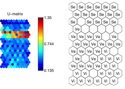
package. TheU-Matrix [17] proposes a distance based map, meant to visualise the

(29)

2.4. The neurones are represented as hexagons, and for each pair of neurones another

hexagon is placed, which reflects their distance . The colour bar at the right of the map represents the distance scale values.

U₋matrix

0.135 0.744 1.35 Labels Se Se Se Ve Ve Ve Ve Ve Ve Vi Vi Se Se Ve Ve Ve Ve Vi Vi Se Se Se Ve Ve Ve Ve Ve Vi Se Se Se Ve Ve Ve Vi Ve Vi Vi Se Se Se Ve Vi Vi Vi Vi Vi Se Se Se Ve Ve Vi Vi Vi Vi

Figure 2.4: U-matrix and respective labelling using the iris data set.

The figure demonstrates a characteristic of the U-Matrix that is the visual identifica-tion of clusters. In this case, it is clear the top region has a red line (which represents high

distance values) of hexagons that sets a border between the speciesetosa andversicolor.

The same cannot be said between versicolor and virginica that seem to collide in some

cases. In summary the U-Matrix gives a perception about the neurones distance between them, that for this study may become useful to verify the distant result of an organised document map. The component plane is a method to visualise the neurones weight

val-Sepal Length

d 4.67 5.97

7.26 Sepal Width

d 2.45 3.18 3.91

Petal Length

d 1.41 3.74

6.07 Petal Width

d 0.185 1.22 2.25

Figure 2.5: Component Planes for the Iris data set.

ues of a specific attribute. For instance, in figure2.5illustrates the weight values map for

(30)

the attribute values in different areas of the map.

There are other visual methods to extract information about the neural network. For

instance in [18,19,20] illustrates several types of projections, where each of them displays

distinct information about the same network. Some of these tools can be used during the dissertation for an analysis over the document map.

lawn green green-yellow

pale green pale-goldenrod antique-white papaya-whip linen old lace beige floral white khaki light-goldenrod moccasin wheat mint cream alice blue ghost white white

dark-sea green dark khaki

burlywood tan

light pink

pink thistle lavender

dark salmon rosy brown plum pale turquoiselight blue

powder blue

dark orange goldenrod

coral

sandy brown light coral hot pink

orchid

violet sky blue

salmon

pale-violet red medium-orchid

medium-purple

chocolate

dark-goldenrod indian red

medium-violet red violet red

dark orchid dark violet

purple blue violet

maroon slate blue

olive drab sienna _firebrickbrown slate gray steel blue cornflower-blue royal blue

dark

olive-green dark slate-blue

cadet blue medium

sea-green

forest green

lime green dark green black

midnight-blue navy blue light sea-green medium-turquoise turquoise dark-turquoise

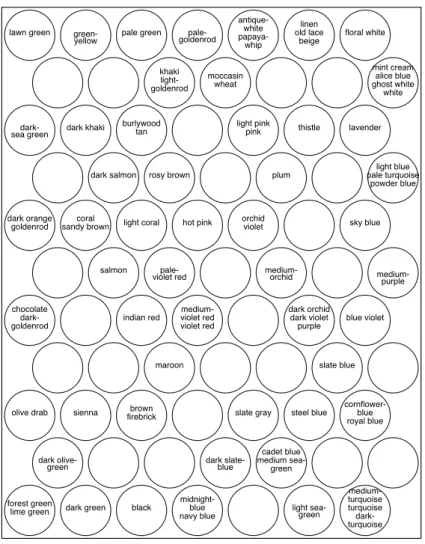
Figure 2.6: A map of colours based on their RGB values.

For the present thesis, we intended to achieve a result similar to the map colours

presented in [21], where a neural network is trained to project an organised map about

different types of colours. In figure2.6 we illustrate the projection result, where similar

colours are either close or located in the same area. There are many research articles [22]

about SOM that use it as a tool to solve scientific and real-word problems. In section2.3,

the combination of textual data with of the SOM algorithm, known as WEBSOM [23], is

(31)

2. RELATEDWORK 2.2. Document Clustering

Self-organised maps handles well a high-dimensional space, which occurs in the doc-uments characterisation. This algorithm matches the document map goal of this study, because the documents are projected into a context map in which they are organised and grouped according to their topics. However, this algorithm requires us to prepare the documents into a supported input structure. In the next section, document data repre-sentation and document clustering for textual-data is analysed.

2.2 Document Clustering

Document clustering finds applicability for a number of tasks: in document organisation and browsing, for efficient searching; in corpus summarisation, providing summary in-sights into the overall content of each cluster of the underlying corpus; and in document classification, since after clusters are built during a training phase, new documents can be classified according to the clusters that were learnt.

Many classes of algorithms such as the k-means algorithm, or hierarchical algorithms are general-purpose methods, which can be extended to any kind of data, including text data. A text document can be represented either in the form of binary data, when using the presence or absence of a word in the document in order to create a binary vector. In such cases, it is possible to directly use a variety of categorical data clustering algorithms

[24, 25, 26] on the binary representations. Although, a more enhanced representation

may include refined weighting methods based on the frequencies/probabilities of the individual words in the document as well as frequencies of words in an entire collection

(e.g., TF-IDF weighting [27]). Quantitative data clustering algorithms [28,29,30] can be

used in conjunction with these weightings in order to determine the most relevant terms in the data to form clusters.

Naive techniques do not typically work well for clustering text data. This is due to the fact that text representation data uses a very large number of distinguishing charac-teristics. In other words, the lexicon associated to the documents may be of the order of

105, though a single document may contain only a few hundred words. This problem

may be more serious when the documents to be clustered are very short such as tweets, for example.

While the lexicon of a given corpus of documents may be large, the words are typi-cally correlated with one another. This means that the number of concepts (or principal components) in the data is much smaller than the feature space. This demands for

algo-rithms that can account for word correlations, such as [31] for example. Nevertheless, if

only single words are used, part of the semantic sharpness of the document content is lost, which may lead to clustering errors. As an example, since the word "coordinates"

has more than one meaning (e.g.he coordinates the projectvsmap coordinates) it may leads

(32)

characterise documents [31]: "map coordinates" instead of "coordinates", or "bus stop" and "bus address", instead of "bus".

The sparse and high dimensional representation of the different documents has also been studied in the information retrieval literature where many techniques have been proposed to minimise document representation for improving the accuracy of matching

a document with a query [27].

2.2.1 Vector space model

In general, a common representation used for text processing is the vector-space model

(VSM). In the basic version of this model [32], a document is stored as binary vector where

each attribute of the vector corresponds to words of the vocabulary, and the value of an attribute is 1 if the respective word exists in the document; otherwise it is 0. Although the binary vector encoding may be useful in certain frameworks, in other cases it is possible to replace them by real values through a function of the word occurrence frequency that results in a statistical value about the word influence in the document. For that, the

vector-space basedTf-Idf can be used.

2.2.1.1 Tf-Idf

Tf-Idf (Term frequency−Inverse document frequency) is a statistical metric often used in

Information Retrieval (IR) and Text Mining to evaluate how important a termW (word

or multi-word) is to a documentdj in a corpusD. It has the following expression:

Tf−Idf(W, dj) =

f(W, dj)

size(dj)

.log kDk

k{d:W ∈d}k (2.9)

kDk stands for the number of documents of corpus D; k{d : W ∈ d}k means the

number of documents containing term W, and size(dj) is the number of words of dj.

Some authors prefer to use the probability (f(W, dj)/size(dj)) of termW in documentdj

instead of the more commonly used absolute frequency (f(W, dj)), as bias towards longer

documents can be prevented.

2.2.2 Feature Selection and Transformation Methods for Text Clustering

2.2.2.1 Stop Words Removal

The quality of any data mining method such as classification and clustering is highly dependent on the noisiness of the features used in the clustering process. Most authors discard commonly used words such as "the", "by", "of" to reduce the number of features,

thinking they are useless to improve clustering quality. However, these stop words are

(33)

2.2.2.2 Entropy-based Ranking

Setting different weights to words is also used for feature selection in text. The

entropy-based ranking was proposed in [33]. The quality of the term is measured by the entropy

reduction when it is removed. The entropyE(t)of the termtin a collection ofn

docu-ments is defined by:

E(t) =− n

X

i=1

X

j = 1n(Sij.log(Sij) + (1−Sij).log(1−Sij) (2.10)

whereSij ∈[0,1]is the similarity between theith andjth document in the collection

ofndocuments is defined as follows:

Sij = 2−

dist(i,j)

dist . (2.11)

dist(i, j)stands for the distance between the termsiandjafter the termtis removed;

distis the average distance between the documents after termtis removed.

2.2.2.3 Dimensionality Reduction Methods

Feature transformation is a different method in which the new features are defined as a functional representation of the original features. The most common is the

dimensional-ity reduction method [34] in which the documents are transformed to a new feature space

of smaller dimensionality where features are typically a linear combination of the

origi-nal data features. Methods such as Latent Semantic Indexing (LSI) [35] use this common

principle. The overall effect is to remove many dimensions in the data which are noisy or partially redundant for similarity based applications such as clustering. LSI is closely

related to the problem of Principal Component Analysis (PCA). For ad-dimensional data

set, PCA builds a symmetricd×dcovariance matrixCof the data, such that each(i, j)th

cell of C is the covariance between dimensions i and j. This matrix is positive

semi-definite and can be decomposed as follows:

C=P . D . PT (2.12)

P is a matrix whose columns contain orthonormal eigenvectors ofCandDis a

diag-onal matrix containing the corresponding eigenvalues. The eigenvectors represent a new orthonormal basis system along which the data can be represented. Each eigenvalue corresponds to the variance of the data along each new dimension. Most of the global variance is preserved in the largest eigenvalues. Therefore, in order to reduce the dimen-sionality of the data, a common approach is to represent the data in this new basis system, which is further truncated by ignoring those eigenvectors for which the corresponding eigenvalues are small. LSI is quite similar to PCA except that uses it approximation of

the covariance matrixCwhich is quite appropriate for the sparse and high-dimensional

(34)

the(i, j)th entry is the normalised frequency for termjin document i. It can be shown

that AT_·_A _{is a} _d_×_d_{matrix and it would be the same as a scaled version (by factor} _n₎

of the covariance matrix, if the data is mean-centred. As in the case of numerical data,

LSI uses eigenvectors ofAT_·_A_{with the largest variance in order to represent the text. In}

typical collections, only about 300 to 400 eigenvectors are required for the representation. If original attributes used in LSI are based only on single words frequencies, the finer granularity of the words polysemy may be lost.

The random mapping [36] is a faster reduction method, compared to LSI and PCA,

to reduce a high-dimensional onto a much lower-dimensional space. However, this ap-proach usually has a greater loss of information than LSI and PCA. The random

projec-tion is formed by multiplying the original matrixMby a random matrixR,

N =M . R , (2.13)

whereN is the reduced projection and its dimensionality is much smaller than the

orig-inal input dimensionality. The random matrix sets for each column a fixed number of randomly distributed ones and the rest of the elements are zeros. The size of random features varies depending on the original matrix, in which the lower-dimension has to be sufficiently orthogonal to provide an approximation of the original features. Although the random mapping method may seem simple it has been successful to reduce the

doc-uments high-dimension into a lower-dimension space [37,38], to later be organised onto

a document map. Further details concerning random mapping properties are presented in [36].

2.2.3 Distance-based Clustering Algorithms

Distance-based clustering algorithms are designed by using a similarity function to

mea-sure the similarity between text objects. One of the most popular meamea-sures is thecosinesimilar

function:

cosine(U, V) =

Pk

i=1f(ui. f(vi

q Pk

i=1f(ui)2.

q Pk

i=1f(vi)2

(2.14)

whereU = (f(u1). . . f(uk))andV = (f(v1). . . f(vk)). Other similarity functions include Pearson correlation and other weighting heuristics and similarity functions. TF-IDF is

used in [39]; BM25 term weighting is used in [40].

Hierarchical Clustering-based Algorithms are used in the context in text data in [41,

42,43,44,45,46,47,48]. Limitations associated to Hierarchical Clustering algorithms are

explained in section2.1.1.

Distance-based Partitioning Algorithms are widely used:k-medoid andk-means

clus-tering are used for text context in [49] and [50], for example. The work in [51] uses the

(35)

2. RELATEDWORK 2.3. WEBSOM

2.3 WEBSOM

WEBSOM [52,53] aims to automatically organise an arbitrary free-text collection to

con-vey browsing and exploration of the documents. The method consists of two hierarchical

connected SOMs: in the first SOM, the word histograms5used to characterise documents

are encoded according to their contexts, so that aword category map[54] is developed to

compose word categories (further details in section2.3.1); for the second level, the

docu-ments are encoded according to the word categories developed in the previous level, and

then clustered using the SOM algorithm. Figure2.7presents an overview of the original

WEBSOM architecture.

preprocessing

self−organization of

word category map

word category

map

self−organization of

document map document encoding

document map

documents documents

Figure 2.7: The original WEBSOM architecture.

2.3.1 Word Category Map

Documents tend to use different terms to describe the same topic. This occurs because each author has his own writing style, so when they compose a document, the topics are described in their manner. This results in a large vocabulary dimension and as documents

are represented by the VSM (section2.2.1), expressions with similar meaning are indexed

as distinct from one to another. The WEBSOM encodes words according to their average

context, in order to develop a SOM about word categories [21,55]. The average context is

(36)

represented by the vectorxi(d), which denotes a statistical description of the words that

occur at neighbourhood dfrom the word i. For a set of displacements{d1, . . ., dn}, the

average context of wordiis

xi =

   

xid1 .. .

xidn

   

. (2.15)

Usually the contextual information is computed for two displacements, the preceding

wordxi−1and succeeding wordxi+1. There are different possibilities to encode the word

contextxid. For instance in [56], the context of wordiat the distancedis encoded as the

vector

xi(d)=

1

|Ii(d)|

X

k∈Ii(d)

ek, (2.16)

whereek stands for the unit vector of the wordk. Ii(d) is the set of words at distanced

from wordiand|Ii(d)|means the size of this set. This encoding has an inconvenience due

to the high dimensionality of the vocabulary. In order to reduce the dimension, the unit

vectorekis replaced by ar-dimensional random vectorrk(section2.2.2.3), which results

in

xi(d) =

1

|Ii(d)|

X

k∈Ii(d)

rk, (2.17)

where therdimension has to be sufficiently orthogonal to provide an approximation of

the original basis. For instance, for the case study [2] it reduced from 39 000 to a 1000

dimensions. Another study at [56] reduced the dimension from 13 432 to 315. So as we

can see the dimension varies according to the original dimension. Random mapping has

been successful [2,56,3,57,37,58] to reduce the size of features when encoding the word

category map, with small loss of information.

Figure 2.8: Case study in [1]: A Usenet Newsgroup.

The case study in [1], organised approximately 12∗105 words into 315 word

(37)

presents a very large dimension reduction, and the categories presented in the figure seem good samples. However, building categories can result in a loss of semantic sharp-ness and ambiguity. For instance, the category composed by the set of countries ("usa", "japan","australia", "china", "israel" ) represent those elements as one, so in a further in-dexing these words are indexed as the same. For this dissertation we aim to solve am-biguity by introducing multi-word expressions (MWEs) and using a different dimension reduction, so that there is no loss of semantic sharpness.

2.3.2 Document Map

Documents are encoded by locating their word histograms in the word category map. For this encoding, each document is represented by the VSM, however, instead of single words the components are word categories. The category weight can be set by the

in-verse frequency of occurrence or some other traditional method [59]. In some WEBSOM

case studies [57,60,53,3], the entropy-based weight (section2.2.2.2) is used to index the

category values. Once the encoding is completed, the document map is formed with the

SOM algorithm using the categories asfingerprintsof the documents.

The WEBSOM method has successfully formed document map for different types of

free-text collections [1,2,52,53,56,3,57,37]. Some of these publications are implemented

at [61] in a demo version to browse and explore the document map. The largest

docu-ment map [3] had approximately 7 million patent abstracts written in English, where the

average length of each text was around 132 words. The document map took around six weeks to be computed, even with the reduction methods applied. The result had the documents ordered meaningfully on a document map according to their contents. For computational reasons, the present dissertation aims to perform a document map for

smaller collections, as was done in [1,52,37].

The case study in [2] organised a collection of 115 000 articles from the Encyclopaedia

Britannica. Thecorpuswas preprocessed to remove unnecessary data, which resulted in

an average length of 490 word per document and a vocabulary of 39 000 words. In this particular study, the word category map was ignored, having the document encoded as a random projection of word histograms. The random projection consisted in a dimension of 1000 features and the number of ones in each column of the sparse random projection

matrix was three. In figure2.9we can visualise a sample of the document map. Although

the word category map step was ignored, the result continues to organise documents according to their contents. This case study result exemplifies one of the motivating factors for this thesis that is to use the WEBSOM method without using the word category map.

2.3.3 Browsing The Document Map

(38)

guira

Hawaiian honeycreeper siskin

kingbird chickadee cacique

bird, yellow, species, black, kingbird, hawaiian, bill, inch, family, have

Descriptive words:

Articles:

chondrichthian : General features leopard shark

soupfin shark shark

fox shark

Articles:

glowworm bagworm moth

caddisfly : Natural history damselfly

lacewing

neuropteran : Natural history mantispid

strepsipteran

homopteran : Formation of galls

shark, fish, species, ray, many, water, feed, have, attack, use

insect, adult, lay, other, water larva, egg, female, species, aphid,

Articles:

bull shark

Cambyses I

chondrichthian : Natural history blacktip shark

shark : Hazards to humans. shark : Description and habits. chondrichthian : Economic value of rays

(39)

document database [52]. If the map is large, subsets of it can first be viewed by

zoom-ing [3], as shown in figure 2.9. To provide guidance for the exploration, an automatic

labelling method (section 2.3.3.1) has been applied to rank keywords for different map

regions [62]. Figures2.9and2.10are examples using the automatic labelling. In addition,

some WEBSOM examples are available for browsing at [61].

2.3.3.1 Automatic labelling

In order to convey an intuitive manner for browsing one needs descriptive "landmarks" to be assigned to the document map regions where particulars topics are discussed. The

automatic labelling [62] is based on two statistical properties: the words occurrence in

the cluster; and the words occurrence in the collection. The goodness of a wordwin a

clusterjis measure by

G(w, j) =F(w, j)PF(w, j)

iF(w, i)

, (2.18)

whereF(w, c)stands for the frequency of the wordwin a clusterc. Based on the previous

equation, the words which occur in the cluster are ranked, and then the top one is denoted as the representative of the cluster. However, the top words are still considered and

ranked, as we can visualise in figure2.9. The labelling is an useful tool to provide an

overview about the most relevant keywords that occur in a cluster or region of the map. In addition, if the keywords have a strong meaning they can give a perception of the main topics.

2.3.3.2 Content Addressable Search

The content addressable search is a method that processes the content text into a docu-ment vector in the same manner as done in the data preparation. The resulting vector is then compared with the model vectors of all map units, and the best-matching units are computed and then saved. The output ranking is an ordered list about the most similar items between the content text and model vectors. This method is often used to visualise where new textual information will be located in the document map.

2.3.3.3 Keyword Search

The keyword search is also a good method for searching the document map. After build-ing the map for each word the map units that contain the word are indexed. Given a search description, the matching units are found from the index and the best matches

are saved. The ranking is then computed according to the best matches. In figure2.10

(40)

2. RELATEDWORK 2.4. Keyword Extractor

Analyzer of speech in noise prone environments Speech decoding apparatus and method of decoding Speech recognizer having a speech coder for an

Method of and system for determining the pitch in human speech A method of coding a speech signal

Low bit rate speech coding system and compression

Method for testing speech recognisers and speaker Speech recognition device

Speech analysis method and apparatus Speaker adapted speech recognition system Speech input device in a system of computer recogn Single picture camera with image and speech encod Speech adaptation system and speech recognizer

speech, signal, code, noise (a) speech, input, recognition, pattern (b) Descriptive words:

speech recognition

Keyword search:

Figure 2.10: Case study in [3]

2.4 Keyword Extractor

For this thesis study we intend to characterise documents by multi-word expressions (MWEs), instead of single words. The reason relies on the ambiguity of single words

which can be solve when using MWEs. For instance, [63] demonstrates that the lemma

worldhas nine different meanings andrecordhas fourteen, while the MWE world record has only one. In addition, when using indexed relevant MWEs, the system accuracy

improves [64]. Section2.4.1gives a brief survey about MWE extractors and section2.4.2

presents a detailed description about the MWEs extractor used in this dissertation.

2.4.1 Multi-Word Expressions Extractors

Regarding multi-word expression extractors, there arelinguisticandstatisticalapproaches.

Linguistic approaches like [65,66,67,68,69,70,71] use syntactical filters, such as

Noun-Noun,Adjective-Noun,Verb-Noun, etc., to identify or extract MWEs. Since the textual data has to be morphosyntactically tagged, this requirement imposes a language dependency on linguistic approaches. Not all languages have high quality taggers and parsers avail-able, especially when languages are unknown. Furthermore, the MWEs relevance is not assured by morphosyntactic patterns. For example, "triangle angle" and "greenhouse

(41)

relevant.

Statistical approaches are usually based on the condition that many of the words of

a MWEs areglued. For example, there is a high probability that in texts, after the word

Barack, appears the wordObama, and that beforeObamaappears the wordBarack. Several

statistical measures, such asMutual Information[72],Coefficient[73],Likelihood Ratio[74],

etc., have been used to obtain MWEs. The problem with these measures is that they only

extract bigrams (sequences of only two words). However, in [75] proposes other metrics

and an extraction algorithm (section 2.4.2), to obtain relevant MWEs of two or longer

words. For this dissertation, a statistical approach is used to obtain MWEs according to their relevance in the collection. Besides, statistical methods are independent from the language which is useful to test this study approach on different languages, in specific Portuguese and English documents.

2.4.2 LocalMaxs

Three tools working together, are used for extracting MWEs from any corpus, the Local-Maxs algorithm, the Symmetric Conditional Probability (SCP) statistical measure and the Fair Dispersion Point Normalization (FDPN).

For a simple explanation, let us consider that a n-gram is a string of n consecutive

words. For example the wordpresidentis an1-gram; the stringPresident of the Republicis

a4-gram. LocalMaxs is based on the idea that eachn-gram has a kind ofglueor cohesion

sticking the words together within then-gram. Differentn-grams usually have different

cohesion values. One can intuitively accept that there is a strong cohesion within then

-gram (Barack Obama) i.e. between the wordsBarackandObama. However, one cannot say

that there is a strong cohesion within then-gram (or uninterrupted) or within the (of two).

So, theSCP(.)cohesion value of a generic bigram (x y) is obtained by

SCP(x y) =p(x|y). p(y|x) = p(x y) p(y) .

p(x y) p(x) =

p(x y)2

p(x). p(y) (2.19)

wherep(x y),p(x)andp(y)are the probabilities of occurrence of bigram(x y)and

uni-gramsxandy in the corpus;p(x|y)stands for the conditional probability of occurrence

ofxin the first (left) position of a bigram in the text, given thaty appears in the second

(right) position of the same bigram. Similarlyp(y|x)stands for the probability of

occur-rence ofyin the second (right) position of a bigram, given thatxappears in the first (left)

position of the same bigram.

However, in order to measure the cohesion value of each n-gram of any size in the

corpus, the FDPN concept is applied to theSCP(.)measure and a new cohesion measure,

SCP_f(.), is obtained.

SCP_f(w1. . . wn) =

p(w1. . . wn)2

1

n−1

Pn−1

i=1 p(w1. . . wi).p(wi+1. . . wn)

(42)

where p(w1. . . wn) is the probability of the n-gramw1. . . wn in the corpus. So, any n

-gram of any length is “transformed” in a pseudo-bi-gram that reflects theaverage cohesion

between each two adjacent contiguous sub-n-gram of the originaln-gram. Now it is

pos-sible to compare cohesions fromn-grams of different sizes.

LocalMaxs Algorithm

LocalMaxs [75, 76] is a language-independent algorithm to extract cohesiven-grams of

text elements (words, tags or characters).

Let W = w1. . . wn be an n-gram and g(.) a cohesion generic function. And let:

Ωn−1(W) be the set of g(.) values for all contiguous(n−1)-grams contained in the n

-gramW;Ωn+1(W)be the set ofg(.)values for all contiguous(n+1)-grams which contain

then-gramW, and letlen(W)be the length (number of elements) ofn-gramW. We say

that

W is a MWE if and only if,

for∀x∈Ωn−1(W),∀y∈Ωn+1(W)

(len(W) = 2 ∧ g(W)> y) ∨

(len(W)>2 ∧ g(W)> x+₂ y) .

Then, forn-grams withn≥3, LocalMaxs algorithm elects everyn-gram whose

cohe-sion value is greater than the average of two maxima: the greatest cohecohe-sion value found

in the contiguous(n−1)-grams contained in then-gram, and the greatest cohesion found

in the contiguous(n+1)-grams containing then-gram.

(43)

3

Proposed Approach

3.1 Architecture

In this study we propose a method to characterise documents and then extract new infor-mation based on the characterised dada. The proposed architecture is presented in figure

3.1. The method is designated as the RSOM approach.

Documents

LocalMaxs _Lexicon

Document Encoding

REs Labeling

SOM

Figure 3.1: Proposed Architecture.

(44)

3. PROPOSEDAPPROACH 3.1. Architecture

are computationally heavy for the selected algorithms in the further component. So, the structure produced in the Document Characterisation component includes a reduction of the number of attributes to characterise the documents. This component is explained in

detail in section 3.2. The previous components form the necessary steps to prepare the

(45)

3. PROPOSEDAPPROACH 3.2. Document Information Retrieval

3.2 Document Information Retrieval

3.2.1 Document Characterisation

In this study documents are characterised by features. Most approaches use a great

num-ber of features, usually based on the entire lexicon available in thecorpus, which become

computationally heavy. So, instead of using all elements of the vocabulary in the cor-pus, a different and reduced set of features was calculated for each document. Thus, by using the MWEs it was possible to calculated a similarity matrix between each pair of documents. This way, each document is characterised by a new vector where each

po-sition reflects the similarity between this document and another document of thecorpus.

This corresponds to a strong feature reduction and there is no loss of information since

all MWEs enter in the calculation of the similarity matrix. As an example, from acorpus

with 148 documents used in this dissertation, 5818 MWEs were extracted. The usual form would use all expressions in the vocabulary to represent each document, which in this case would correspond to 5818 features. Instead of this number, there is a compression of 5818 to 148 (the number of documents) and this reduced number of attributes is used

to characterise the same documents. In figure3.2, the left matrix is replaced by the right

matrix,     

w1,1 w1,2 · · · w1,vlen

w2,1 w2,2 · · · w2,vlen

..

. ... . .. ...

wdlen,1 wdlen,2 · · · wdlen,vlen

     ⇒     

s1,1 s1,2 · · · s1,dlen

s2,1 s2,2 · · · s2,dlen

..

. ... . .. ...

sdlen,1 sdlen,2 · · · sdlen,dlen

    

Figure 3.2: Reduction example.

where wk,i means the probability of the attribute i in document k and sk,q stands

for the similarity between documents k and q, which is based in Pearson correlation,

equation 3.1. The vlen denotes the length of the vocabulary and dlen the number of

documents.

sk,q=

cov(k, q)

p

cov(k, k)∗p

cov(q, q) (3.1)

cov(k, q) = 1 vlen−1

i=vlen

X

i=1

(wk,i−wk,.)∗(wq,i−wq,.) (3.2)

wherewk,.means the average value of the attributes for documentkwhich is given by

wk,.=

1 vlen

i=vlen

X

i=1

wk,i . (3.3)

(46)

3. PROPOSEDAPPROACH 3.2. Document Information Retrieval

all MWEs in the corpus and this sum is divided by the number of all elements in the vocabulary.

In Pearson correlation, similarities range from -1 to +1, so ifsk,q is close to 0 it means

that the similarity between documents is weak; if it is close to +1, the similarity betweenk

andqis strong; if negative, it means that documents are dissimilar. This scale is the same

in all cases, which allows comparison of different correlations. In addition, by looking

at(wk,i−wk,.)∗(wq,i−wq,.)in equation3.2, which is the contribution of MWEiin the

result, each product either enhances or penalises the similarity between both documents. The different types of contributions are:

1. wk,i > 0∧wq,i > 0: When MWE i occurs in both documents, the subtractions

(wk,i −wk,.) and (wq,i−wq,.) are positive, because wk,i andwq,i are greater than

the corresponding average values wk,. andwq,.. Being both positive, this product

enhances the similarity between documentsk andq. The impact of this

contribu-tion varies according to the probability of MWEiin both documents, where high

probabilities have a greater weight in the result.

2. (wk,i >0∧wq,i= 0)∨(wk,i= 0∧wq,i >0): Since MWEioccurs in only one of the

documents, the product(wk,i−wk,.)∗(wq,i−wq,.)will be negative because one of

the subtractions is negative and the other is positive. So, the similarity is penalised when the MWE occurs in only one of the documents.

3. wk,i= 0∧wq,i= 0: If a MWE does not occur in either documents, both subtractions

wk,i−wk,. andwq,i−wq,.are negative. So, the product(wk,i−wk,.)∗(wq,i−wq,.)

is simplified towk,.∗wq,., which is a weak positive value. This coherent to the idea

that two documents must be considered strongly similar when they have MWEs in common and weakly similar when they share the absence of MWEs.

In this work, we need a tool to measure the individual contribution of each MWE in

the similarity between documentskandq. As we will see, this is useful to highlight what

are the MWEs responsible for a similarity result. So, based on equation3.1, the individual

contribution is measured by the following metric:

score(M W E, k, q) = (wk,M W Ep −wk,.)∗(wq,M W E−wq,.)

cov(k, k)∗p

cov(q, q) (3.4)

As said before, MWEs are extracted by LocalMaxs that retrieves many relevant ex-pressions. However, this algorithm also extracts terms that are not informative and shouldn’t be considered as good connectors between documents. In order to connect doc-uments based on relevant expressions, MWEs are weighted in a way that strong terms will provide greater similarities and weak term tend to be ignored. Therefore to

deter-mine the weight attribute, the probability of occurrence of MWEiin a documentk(wk,i)