Tracking a cold filament with matched-field inversion

CINTAL - Centro de Investiga¸

c˜

ao Tecnol´

ogica do Algarve

Universidade do Algarve

Tracking a cold filament

with matched-field inversion

V. Corr´

e

Rep 01/02 - SiPLAB 09/July/2002

University of Algarve tel: +351-289800131 Campus da Penha fax: +351-289864258

8000, Faro, [email protected]

Work requested by CINTAL

Universidade do Algarve, Campus da Penha, 8000 Faro, Portugal

tel: +351-289800131, [email protected], www.ualg.pt/cintal

Laboratory performing SiPLAB - Signal Processing Laboratory

the work Universidade do Algarve, FCT, Campus de Gambelas,

8000 Faro, Portugal

tel: +351-289800949, [email protected], www.ualg.pt/uceh/adeec/siplab

Projects ATOMS - FCT, PDCTM/P/MAR/15296/1999

Title Tracking a cold filament with matched-field inversion

Authors V. Corr´e

Date July 09, 2002

Reference 01/02 - SiPLAB

Number of pages 44 (forty four)

Abstract Simulation tests are carried out to estimate the time, range

and depth variations of ocean acoustic properties. The esti-mation is based on matched-field inversion defined by a cou-pled mode acoustic model, a linear misfit function and an hybrid search algorithm. It is shown that tracking cold fila-ments is possible even in non-optimal conditions.

Clearance level UNCLASSIFIED

Distribution list SiPLAB (1), CINTAL (2), FCT (1)

Total number of copies 4 (four)

III

Contents

List of Figures V

1 Introduction 7

2 Parameterization of the environment 8

3 Matched-field inversion 10 3.1 Propagation code . . . 10 3.2 Objective function . . . 10 3.3 Search algorithm . . . 11 4 Simulated study 12 4.1 Ideal case . . . 12 4.1.1 Synthetic data . . . 12 4.1.2 Inversions . . . 12

4.1.3 Effect of middle-cell size and location on the inversion results . . . . 14

4.2 Non-ideal cases . . . 20

4.2.1 Effect of correlated noise on the inversion results . . . 20

4.2.2 Effect of model mismatch on the inversion results . . . 21

4.3 Systematic study . . . 31

5 Conclusion 35 A Description of the files related to sound-speed estimation 37 A.1 Content of the directory . . . 37

A.2 How to run a series of inversions? . . . 38

A.3 List of inversion scenarios . . . 40

B Sample of the csnap.m file 43

List of Figures

2.1 Waveguide model . . . 9

4.1 Spatial variations of the temperature in a region featuring an upwelling filament . . . 13

4.2 Time variations of the sound-speed profiles in the middle cell . . . 15

4.3 Estimated sound-speed profiles in the middle cell . . . 15

4.4 True and estimated range limits of the middle cell . . . 16

4.5 Error between the true and estimated temperature profiles in the middle cell 16 4.6 Variations of the parameter mean relative error with the middle cell location and width . . . 17

4.7 Estimated sound-speed profiles in the middle cell . . . 18

4.8 True and estimated range limits of the middle cell . . . 19

4.9 Estimated sound-speed profiles in the middle cell for SNR=10 and 5 dB . . 22

4.10 True and estimated range limits of the middle cell for SNR=10 and 5 dB . 23 4.11 Error between true and estimated temperature profiles for SNR=10 and 5 dB 24 4.12 Minimum misfit obtained during the inversions for SNR=10 and 5 dB . . . 25

4.13 Sensitivity for SNR=10 and 5 dB . . . 26

4.14 True and estimated sound-speed profiles. 250 m transition cells . . . 27

4.15 True and estimated sound-speed profiles. 500 m transition cells . . . 28

4.16 True and estimated sound-speed profiles. 500 m transition cells . . . 29

4.17 Minimum misfit obtained during the inversions with model mismatch . . . 30

4.18 Variability of the parameter mean relative error with source-array distance 32 4.19 Variability of the parameter mean relative error with array vertical position 32 4.20 Variability of the parameter mean relative error with source depth . . . 33

4.21 Sensitivity for scenario 6 . . . 33 V

VI LIST OF FIGURES

Chapter 1

Introduction

ATOMS is an ambitious project that aims at developing a monitoring system for the Portuguese EEZ using acoustic tomography. A preliminary test for this system is to monitor the recurrent cold filaments/upwellings that develop off of the south west coast of Portugal, using a single vertical array of receivers and a towed source. This paper presents a synthetic study that simulates the monitoring conditions of this particular region and intends to check the feasibility and limits of such a monitoring.

The estimation of range-dependent properties with a single array-source pair is a prob-lem which solution may not be unique. Being aware that this difficulty is particularly true when data are contaminated with noise (i.e., in all real cases), our objective was to obtain a variability trend rather than very accurate estimates of the properties. In other words, detection and global tracking of the filaments were of prime interest rather than detailed mapping of the sea-temperature (or sound-speed) field.

While acoustic travel-time tomography [1] is now a well-developed technique for large-scale, deep-ocean regions, it is less adapted for studying filaments which are mesoscale features that develop in relatively shallow (400 m) areas. Using matched-field processing to estimate ocean sound speed [2, 3] is a more recent approach than tomography. However this approach has already shown good results and can treat any type of environment equally. It is therefore the approach adopted in this study.

This report is organised as follows. The waveguide model chosen to represent the range-dependent environment and the model parameters are defined in the next Section. Section 3 describes the matched-field inversion (MFI) method used to estimate the model parameters. Inversion results obtained for simulated data in ideal and non-ideal (i.e., more realistic) cases are shown in Section 4. Finally, some conclusions are given in Section 5.

Chapter 2

Parameterization of the environment

The parameterization of the ocean environment is a delicate issue since the inversion re-sults depend on the environment model adopted while the form of the real ocean waveguide is usually unknown. An inappropriate model can be a source of mismatch, a situation where the minimum misfit does not correspond to the true ocean properties, and can lead to poor estimates. Usually, independent a priori information guides the choice of the model. When modeling a range-dependent environment, the choice of the model also de-pends on the desired accuracy of the estimates. In our case, since we were first interested in detecting mesoscale ocean features rather than detailed mapping, a coarse model was used to represent the ocean.

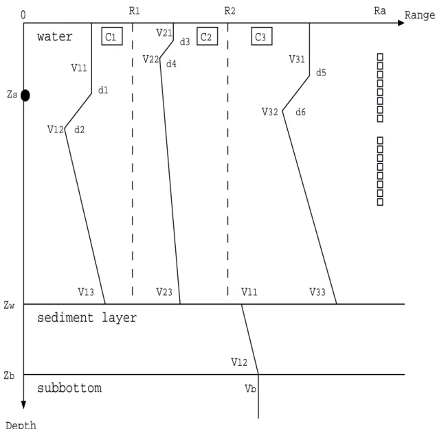
In this model (see fig. 2.1), the water layer is gridded into three vertical cells (C1, C2

and C3) of variable size. Each cell has an independent sound-speed profile and represents

a water mass entity. More specifically, the middle cell represents the water mass with abnormal temperature that we want to estimate. Obviously, this representation would not be a pertinent choice to model an environment which properties vary smoothly and continuously with range. However to detect sharp fronts, such a model appears as a good first approximation. In addition, the use of vertical range limits for the middle cell is a simplification that is not unrealistic when modeling an upwelling since the water mouvement is mainly upwards. The rest of the model consists of a sediment layer laying over a semi-infinite substrate. Each layer (or cell) is characterized by its density, thickness, P- and S-wave velocities and attenuations.

For tomography purposes, the traditional approach to model the sound speed in the water is to use empirical orthogonal functions (EOFs). This method has been increasingly used since it can provide a high accuracy despite only a few coefficients/parameters are required. On the other hand, a major constraint in using EOFs is that one already needs a good knowledge (through direct measurements) of the ocean’s properties to be able to calculate the eigenfunctions. In order to have eigenfunctions that accurately characterize both range and time variability of the sound speed, one needs a relatively large amount of measurements. However, the basic idea behind tomography, or any other remote-sensing method, is precisely to avoid direct measurements as much as possible. Therefore, we chose to estimate sound-speed points rather than EOF coeffcients.

In general, many points are necessary to get a good accuracy of the sound speed. On the other hand, estimating a large number of sound-speed points is an heavy task for an optimization method such as MFI. Once again, considering that our objective was primarily detection rather than accurate mapping of temperature anomalies, we chose a coarse representation of the sound speed that involved few but relevant parameters to

9

estimate. In this representation, the sound-speed profiles are defined with only three points: the sound speed in the homogenous sea-surface layer, at the lower limit of the thermocline and at the seafloor. Between the depth points, the inverse of the sound-speed squared varies linearly with depth.

The parameters to estimate are the three sound speeds of the middle-cell profile. (The sound speeds in the two other cells are suposed to be known.) In order to have a realistic and flexible model, the upper and lower limits of the thermocline (d3 and d4) are also

estimated, as well as the range limits of the middle cell (R1 and R2).

water

sediment layer

subbottom

C

C

C

R

R

Ra

0

Range

Depth

Z

Z

Z

V

V

V

V

V

V

V

V

V

V

V

V

Figure 2.1: Model of the ocean waveguide. The acoustic source is located at range 0, the

Chapter 3

Matched-field inversion

In MFI, the estimation of model parameters consists in determining the optimum set of parameters that minimizes the misfit between the measured pressure field and the modeled field calculated for specific parameter values. This section briefly describes the different components of the MFI: the acoustic propagation code that calculates the mod-eled pressure fields, the cost function that quantifies the misfit, and the search algorithm that samples the parameter space in order to minimize the misfit.

3.1

Propagation code

In order to have a good compromise between accuracy and computational time, all pres-sure fields (simulated data and replica) were calculated using the SACLANTCEN coupled-mode code C-SNAP [4]. C-SNAP divides a range-dependent environment into several range-independent sections and can therefore handle waveguide models such as the one shown in fig. 2.1.

3.2

Objective function

To quantify the misfit between the data and replica fields, the frequency-incoherent

Bartlett processor was used. The processor can be described as follows. Let ˆD(f )

repre-sent the normalized data pressure field measured at frequency f , and ˆP∗(m, f ) represent

the normalized replica field calculated for the model of parameters m. When the fields

have Nf frequency components, the cost function to minimize is given by:

E(m) = 1₋ 1 Nf Nf X k=1 | ˆP∗(m, fk) ˆD(fk)|2. (3.1) 10

3.3. SEARCH ALGORITHM 11

3.3

Search algorithm

Due to the size of the parameter space and the non-linearity of the problem, neither an exhaustive nor a local search (gradient-type search) were a suitable approach to sample the parameter space. Instead an hybrid algorithm, the simplex genetic algorithm (SGA), was used. This algorithm combines the downhill simplex (DHS) [5] and genetic algorithm (GA) [6] for the local and global search respectively; and has shown good performances in previous inversions [7].

Chapter 4

Simulated study

In order to test the inversion method, it was first applied to synthetic data in the ideal case where there was no source of mismatch. It was then applied to more realistic cases when noise was added to the data and when the waveguide models used to calculate the data and replica were different.

4.1

Ideal case

4.1.1

Synthetic data

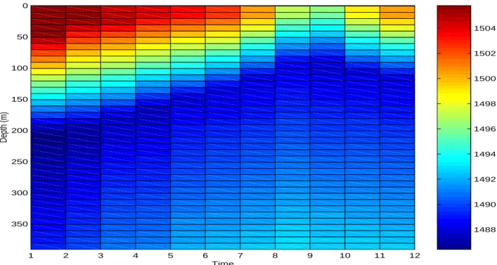
The baseline environmental model used to generate synthetic data sets is illustrated in fig. 2.1. The vertical array was made of two sections of eight receivers. Since the compu-tational time increases linearly with the number of frequencies, the pressure fields were calculated only at 250 and 500 Hz. The value of the time and range-independent pa-rameters of the waveguide are given in tab. 4.1. Synthetic time and range-dependent sound-speed profiles were derived from temperatures and salinities measured in an area featuring a cold filament [8] (see fig.4.1). A total of 11 time windows were selected to represent the apparition and evolution of a cold filament. In the first time window, the sound-speed profiles were identical in all three cells (range-independent ocean). The pro-files of the middle cell are illustrated in fig. 4.2. The propro-files in the two other cells did not

vary with time and were known during the inversion. (In practice, profiles in cells C1 and

C3 can be estimated by measuring the salinity and temperature profiles at the source and

array locations.) The width of the middle cell randomly varied in time within the [11.95 - 12.05 km] interval while the horizontal distance between the source and the middle-cell

front (R1) varied between 10.95 and 11.05 km. With such a geometry, the middle cell was

centered between the source and the array, and its width slightly larger than C1 or C3.

4.1.2

Inversions

The inversion method was applied three times to the data of each time window. Approx-imately 10000 sets of parameters were tested in each inversion with an initial population of 35 random sets. All known parameters of the waveguide were set to their true value (see tab. 4.1) such that, in theory, a global minimum misfit of zero could be reached

4.1. IDEAL CASE 13

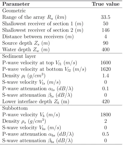
Table 4.1: Time and range-independent parameters

Parameter True value

Geometric

Range of the array Ra (km) 33.5

Shallowest receiver of section 1 (m) 50

Shallowest receiver of section 2 (m) 146

Distance between receivers (m) 4

Source depth Zs (m) 90

Water depth Zw (m) 400

Sediment layer

P-wave velocity at top Vl1 (m/s) 1600

P-wave velocity at bottom Vl2 (m/s) 1620

Density ρl (g/cm3) 1.4

S-wave velocity Vls (m/s) 0

P-wave attenuation αls (dB/λ) 0.1

S-wave attenuation βls (dB/λ) 0

Lower interface depth Zb (m) 420

Subbottom P-wave velocity Vb (m/s) 1800 Density ρs (g/cm3) 2 S-wave velocity Vbs (m/s) 0 P-wave attenuation αbs (dB/λ) 0.5 S-wave attenuation βbs (dB/λ) 0 8 9 10 11 12 13 14 15 0 20 40 60 80 100 120 140 160 180 200 50 100 150 200 Range (km) Depth (m)

Figure 4.1: Spatial variations of the temperature in a region featuring an upwelling fila-ment .

14 CHAPTER 4. SIMULATED STUDY

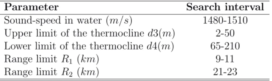
during the inversion. The search intervals were identical in all inversions and are given in tab. 4.2. In practice, the sound speed in the surface layer and at the bottom were defined by positive perturbations of the sound speed at the lower part of the thermocline:

V21= V22+ υ1; V23= V22+ υ2; (4.1)

and υ1 and υ2 were the parameters to estimate rather than V21 and V23. The purpose

of this change of variables was to reduce the number of possible solutions by introducing

meaningful constraints. In practice, the choice of the intervals for the range limits R1 and

R2 would require a priori information such as satellite images of sea-surface temperature.

Table 4.2: Search intervals for the unknown parameters

Parameter Search interval

Sound-speed in water (m/s) 1480-1510

Upper limit of the thermocline d3(m) 2-50

Lower limit of the thermocline d4(m) 65-210

Range limit R1 (km) 9-11

Range limit R2 (km) 21-23

The set of parameters corresponding to the minimum misfit encountered during the three inversions carried out for each time window was considered as the parameter esti-mates. Estimates of the sound-speed profiles and of the range limits of the middle cell are given in figs. 4.3 and 4.4 respectively. The cold-water raising is clearly visible and

the range limits are well estimated. Since the environment is range independent in the

first time window, the range limits are meaningless for this particular window, and so are their estimates (outfitters in fig. 4.4). A more physical representation of the inver-sion results is given in fig. 4.5 which shows the difference between the corresponding true and estimated sea-temperature profiles. The maximum and average absolute error (over

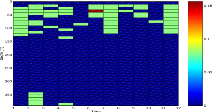
depth and time) are less than 0.16 and 0.02◦C respectively. (The absolute temperatures

in the profiles range between 7.5 and 13◦C.) These results show that, for this particular

configuration, it is possible to not only detect the cold water upwelling but also to obtain an accurate mapping of the sound-speed/temperature profile. However, regarding the temperature estimate, one has to take into account that the temperature profiles were de-duced from the estimated sound-speed profiles and the exact salinity profiles. In practice, an error of 1 % in salinity (i.e., approximately the difference introduced by the filament)

would lead to a temperature error of 0.4◦C. Therefore temperature estimates must be

handled carefully. It is worth noting that the misfits corresponding to these estimates

were small (between 10−6 and 10−4) but were not the global minimum, i.e., the machine

accuracy 10−16. Considering that 1) the parameter accuracy was already relatively good

for misfits between 10−6 and 10−4, 2) misfits smaller than 10−4 were unexpected in

realis-tic scenarios, and 3) we were mainly interested in global detection rather than accuracy, we kept the number of iterations equal to 10000 in the rest of the study. Each inversion was then 45 minutes long approximately.

4.1.3

Effect of middle-cell size and location on the inversion

results

The sensitivity of the pressure field to the sound-speed/temperature anomaly, and there-fore the performance of the inversion method, vary with the properties of the anomaly:

4.1. IDEAL CASE 15 1488 1490 1492 1494 1496 1498 1500 1502 1504 1 2 3 4 5 6 7 8 9 10 11 12 0 50 100 150 200 250 300 350 Depth (m) Time

Figure 4.2: Time variations of the sound-speed profiles in the middle cell. These profiles define the true environment.

1488 1490 1492 1494 1496 1498 1500 1502 1504 1 2 3 4 5 6 7 8 9 10 11 12 0 50 100 150 200 250 300 350 Depth (m) Time

16 CHAPTER 4. SIMULATED STUDY 1 2 3 4 5 6 7 8 9 10 11 10 12 14 16 18 20 22 24 Time Range (km)

Figure 4.4: True (circle) and estimated (star) range limits of the middle cell.

0 0.05 0.1 0.15 1 2 3 4 5 6 7 8 9 10 11 12 0 50 100 150 200 250 300 350 Depth (m) Time

Figure 4.5: Absolute error between the true and estimated temperature profiles in the middle cell.

4.1. IDEAL CASE 17

dimension, location and sound-speed itself. To illustrate the effect of these properties, series of inversions were repeated for three sizes of the middle cell (12, 7 and 2 km) and

three locations (R1=5, 11 and 17 km from the source). From one inversion to another, all

other parameters were identical, including the inversion parameters (number of iterations, size of GA population etc...). For each inversion, the parameter mean relative error ε was calculated according to Eq. 4.2:

ε = 1 Np Np X p=1 |m(p) − mt(p)| mt(p) , (4.2)

where Np is the number of parameters (Np =7 here), m(p) is the estimate of the pth

parameter and mt(p) is its true value. The variations of the error with time for all cases

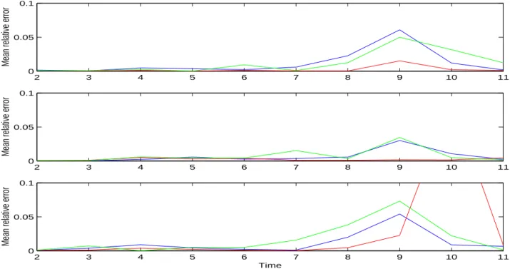
are given in fig. 4.6. The general observation is that the parameter estimates degrade for the time windows 8, 9 and 10 which correspond to the cases where the homogenous sea-surface layer is very thin (<8 m). Then, the results show that for identical inversion conditions the best performance of the inversion method is obtained when the middle cell is centered between the source and the array. This region is most likely to have the best sampling in terms of acoustic energy. The effect of the cell width is less clear as the 12 km and 2 km cases gave similar variations. However, in any case, it is possible to obtain a very good approximation of the filament evolution (see figs. 4.7 and 4.8).

2 3 4 5 6 7 8 9 10 11

0 0.05 0.1

Mean relative error

2 3 4 5 6 7 8 9 10 11

0 0.05 0.1

Mean relative error

2 3 4 5 6 7 8 9 10 11

0 0.05 0.1

Mean relative error

Time

Figure 4.6: Variations of the parameter mean relative error (ε) with the middle cell

loca-tion (top: R1=5 km, middle: R1=11 km, bottom: R1=17 km) and width (blue: 12 km,

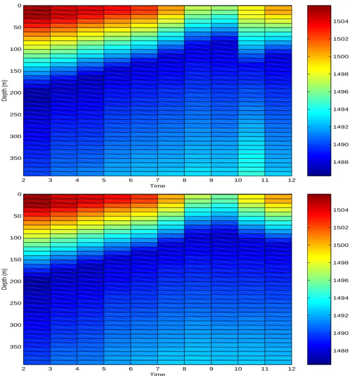
18 CHAPTER 4. SIMULATED STUDY 1488 1490 1492 1494 1496 1498 1500 1502 1504 2 3 4 5 6 7 8 9 10 11 12 0 50 100 150 200 250 300 350 Depth (m) Time 1488 1490 1492 1494 1496 1498 1500 1502 1504 2 3 4 5 6 7 8 9 10 11 12 0 50 100 150 200 250 300 350 Depth (m) Time

Figure 4.7: Estimated sound-speed profiles in the middle cell located 17 km from the source and with a width of 7 km (top) and 2 km (bottom). The true profiles are given in fig. 4.2.

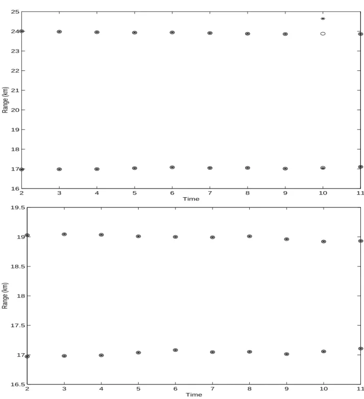
4.1. IDEAL CASE 19 2 3 4 5 6 7 8 9 10 11 16 17 18 19 20 21 22 23 24 25 Time Range (km) 2 3 4 5 6 7 8 9 10 11 16.5 17 17.5 18 18.5 19 19.5 Time Range (km)

Figure 4.8: True (circle) and estimated (star) range limits of the middle cell located 17 km from the source.

20 CHAPTER 4. SIMULATED STUDY

4.2

Non-ideal cases

In reality, ideal cases such as the one treated above do not occur. Therefore, it is important to know the limitations of the inversion method for more realistic conditions. Here we investigate two potential sources of mismatch: the presence of noise in the data and an erroneous parameterization of the waveguide. These situations imply a non-null global minimum misfit and the fact that this global minimum may not correspond to the true parameters. Since MFI works as a “black box” where the inversion is only driven by minimizing the misfit function, a case-by-case study is necessary to know the effect of a particular mismatch on the parameter estimates.

4.2.1

Effect of correlated noise on the inversion results

Correlated noise N(f ) was added to the original synthetic pressure field P(m, f ) to

gen-erate a new data set P0(m, f ) according to:

P0(m, f ) = P(m, f ) + K_{· N(f),} (4.3)

where K is a vector of real numbers that allows to set the level of noise at each hydrophone h to a given value (see Eq. 4.6). The noise itself was a sum of two components:

Nh(f ) = α(f ) + βh(f ), (4.4)

where α(f ) and βh(f ) were complex, zero-mean, Gaussian-distributed random numbers.

The fact that for a given frequency, the pressure fields at all hydrophones contained an identical component (α) increased the degree of correlation between the pressure fields. On the other hand, β simulated the white-noise component (ambient noise) of the measured

pressure fields. Let σαand σβbe the standard deviations of α and β. The noise correlation

between hydrophones h and j is given by:

Chj(f ) = E[Nh(f )Nj∗(f )]

= E[(α(f ) + βh(f ))(α(f ) + βj(f ))∗]

= E[(α(f )α∗(f ))] + E[βh(f )βj∗(f )]

+E[βh(f )α∗(f )] + E[α(f )βj∗(f )]

(4.5) Since α and β are independent noise realizations, the last two terms are nul and the

correlation is reduced to Chj(f ) = σα for j 6= h, and Chh(f ) = σα+ σβ for j = h. In

practice, σα and σβ were set equal.

The performance of the inversion method was tested for two levels of noise: 10 and

5 dB, the signal-to-noise ratio (SNR) at the hth _{hydrophone being defined by:}

SNRh = 10× log10   PNf i=1|Ph0(m, fi)|2 PNf i=1|Nh(fi)|2  . (4.6)

Inversions were carried out for a middle cell located 11 km from the source and with a width of 12 km. Except for the presence of the noise, the conditions of inversion were the same than for the ideal case. For a given SNR and time window, five different noisy data

4.2. NON-IDEAL CASES 21

sets were inverted. Estimates of the sound-speed profiles and range limits obtained with the smallest misfit out of these five inversions are shown in figs. 4.9 and 4.10 respectively. For comparison, the differences between estimated and true sea-temperature profiles are shown in fig. 4.11. The larger the noise, the larger the differences. The mean absolute error

over depth and time is 0.056 and 0.126◦C for 10 and 5 dB respectively. However, despite

the presence of noise, the parameter estimates are relatively good and the evolution of the cold filament can still be well observed.

Since the global minimum is unknown, it is not possible to know if the inversion algo-rithm has reached it or not. One can only verify that the minimum misfit encountered is smaller than the misfit calculated for some particular parameter sets. Here, one obvious set to check is the set of true parameters, i.e., the parameters used to generate the noise-free pressure fields. As shown in fig. 4.12, the misfit calculated with the true parameters is not null and is larger than the minimum misfit encountered for each time window. Standing by itself, this result only stresses the ability of the inversion algorithm to reach regions of low misfit. However the sensitivity curves obtained for the ideal and 5dB cases (see fig. 4.13) provide additional insight in the problem as the two series of curves have very similar behavior and exhibit their global minimum at the parameter true values. Al-though the generalization to the entire parameter space (multi-dimensional space) is not feasible here, this result can explain the relative robustness of the parameter estimates to the presence of noise in the data.

4.2.2

Effect of model mismatch on the inversion results

In the above, the waveguide models used to calculate the simulated data and replica fields had the same geometry (three layers, three cells, flat bottom etc...). Here we are interested in increasing the complexity of the water layer in the true waveguide, while keeping the original parameterization of the replica waveguide in order to test the inversion method in a more realistic scenario. Among the possible approaches to make the waveguide more complex, we chose to introduce transition cells on each side of the middle cell. The

parameters of these cells were set to average values between the middle cell and C1 or

C3’s parameters. The width of the transition cells varied between 250 and 750 m. The

transition cells were overlapping the middle cell in the sense that C1 and C3 always had

a constant width of 10 and 13 km respectively. The search intervals for the range limits were increased to 3 km wide to include the transition cells. Estimated profiles are given in figs. 4.14 to 4.16. The wider the transition cells, the larger the error in the middle-cell profile estimate. Here again, the error is larger for the time windows 8, 9 and 10. However, up to 500 m wide, the global picture of the cold water upwelling is well visible.

As for the noise case, the global minimum is unknown in all scenarios. However here, it is not possible to use the true parameters to verify the algorithm convergence to a low misfit region since the replica waveguide is defined by less parameters than the true waveguide. Nevertheless, for comparison purpose, a reference misfit was calculated with the true parameters of the middle cell. As shown in fig. 4.17, this reference is relatively large and always larger that the minimum misfit encountered during the series of inversions, indicating a good performance of the algorithm to reach regions of low misfit.

22 CHAPTER 4. SIMULATED STUDY 1488 1490 1492 1494 1496 1498 1500 1502 1504 2 3 4 5 6 7 8 9 10 11 12 0 50 100 150 200 250 300 350 Depth (m) Time 1488 1490 1492 1494 1496 1498 1500 1502 1504 2 3 4 5 6 7 8 9 10 11 12 0 50 100 150 200 250 300 350 Depth (m) Time

Figure 4.9: Estimated sound-speed profiles in the middle cell for SNR=10 (top) and 5 dB (bottom). The true profiles are given in fig. 4.2.

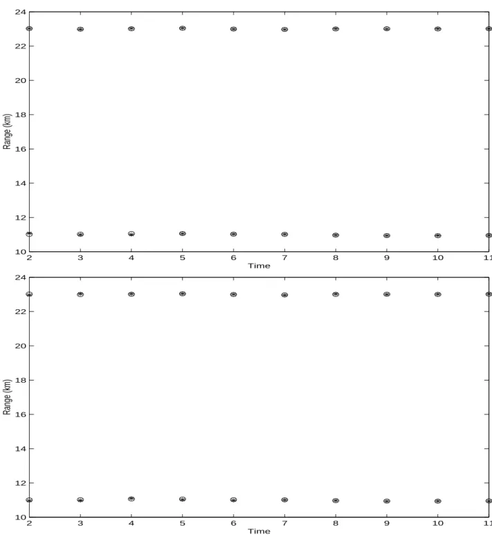
4.2. NON-IDEAL CASES 23 2 3 4 5 6 7 8 9 10 11 10 12 14 16 18 20 22 24 Time Range (km) 2 3 4 5 6 7 8 9 10 11 10 12 14 16 18 20 22 24 Time Range (km)

Figure 4.10: True (circle) and estimated (star) range limits of the middle cell for SNR=10 (top) and 5 dB (bottom).

24 CHAPTER 4. SIMULATED STUDY 0 0.05 0.1 0.15 0.2 0.25 0.3 2 3 4 5 6 7 8 9 10 11 12 0 50 100 150 200 250 300 350 Depth (m) Time 0 0.05 0.1 0.15 0.2 0.25 0.3 0.35 0.4 0.45 0.5 2 3 4 5 6 7 8 9 10 11 12 0 50 100 150 200 250 300 350 Depth (m) Time

Figure 4.11: Absolute error between true and estimated temperature profiles for SNR=10 (top) and 5 dB (bottom).

4.2. NON-IDEAL CASES 25 2 3 4 5 6 7 8 9 10 11 0 0.02 0.04 0.06 0.08 0.1 0.12 0.14 0.16 0.18 0.2 Misfit Time 2 3 4 5 6 7 8 9 10 11 0 0.05 0.1 0.15 0.2 0.25 0.3 0.35 0.4 Misfit Time

Figure 4.12: Minimum misfit obtained during the inversions for SNR=10 (top) and 5 dB (bottom). The circles indicate the misfit calculated with the true parameters.

26 CHAPTER 4. SIMULATED STUDY 14800 1490 1500 1510 0.5 1 V21 (m/s) 14800 1490 1500 1510 0.5 1 V22 (m/s) 14800 1490 1500 1510 0.5 1 V23 (m/s) 10 20 30 40 50 0 0.5 1 d3 (m) 100 150 200 0 0.5 1 d4 (m) 10.5 11 11.5 12 0 0.5 1 R1 (km) 22.5 23 23.5 24 0 0.5 1 R2 (km)

Figure 4.13: Variations of the misfit with individual parameter, the remaining parameters being fixed to their true value for time window 4, cell width 12 km and distance from source 11 km. The dash line indicates the noise-free case. The solid line shows the average misfit obtained for 15 realizations of correlated noise with SNR=5dB.

4.2. NON-IDEAL CASES 27 0 50 100 150 200 250 300 350 Time 2 Depth (m) 10 15 20 0 50 100 150 200 250 300 350 Range Depth (m) Time 3 10 15 20 Range Time 4 10 15 20 Range Time 5 10 15 20 Range Time 6 10 15 20 Range Time 7 10 15 20 Range Time 8 10 15 20 Range Time 9 10 15 20 Range Time 10 10 15 20 Range 1490 1495 1500 1505 Time 11 1490 1495 1500 1505 10 15 20 Range

Figure 4.14: Time variations of the true (top) and estimated (bottom) sound-speed profiles. Transitions cells are 250 m wide. Note that for clarity and emphasis on the middle cell

28 CHAPTER 4. SIMULATED STUDY 0 50 100 150 200 250 300 350 Time 2 Depth (m) 10 15 20 0 50 100 150 200 250 300 350 Range Depth (m) Time 3 10 15 20 Range Time 4 10 15 20 Range Time 5 10 15 20 Range Time 6 10 15 20 Range Time 7 10 15 20 Range Time 8 10 15 20 Range Time 9 10 15 20 Range Time 10 10 15 20 Range 1490 1495 1500 1505 Time 11 1490 1495 1500 1505 10 15 20 Range

Figure 4.15: Time variations of the true (top) and estimated (bottom) sound-speed profiles. Transitions cells are 500 m wide.

4.2. NON-IDEAL CASES 29 0 50 100 150 200 250 300 350 Time 2 Depth (m) 10 15 20 0 50 100 150 200 250 300 350 Range Depth (m) Time 3 10 15 20 Range Time 4 10 15 20 Range Time 5 10 15 20 Range Time 6 10 15 20 Range Time 7 10 15 20 Range Time 8 10 15 20 Range Time 9 10 15 20 Range Time 10 10 15 20 Range 1485 1490 1495 1500 1505 Time 11 1485 1490 1495 1500 1505 10 15 20 Range

Figure 4.16: Time variations of the true (top) and estimated (bottom) sound-speed profiles. Transitions cells are 750 m wide.

30 CHAPTER 4. SIMULATED STUDY 2 3 4 5 6 7 8 9 10 11 0 0.1 0.2 0.3 0.4 0.5 0.6 0.7 0.8 0.9 1 Misfit Time 2 3 4 5 6 7 8 9 10 11 0 0.1 0.2 0.3 0.4 0.5 0.6 0.7 0.8 0.9 1 Misfit Time 2 3 4 5 6 7 8 9 10 11 0 0.1 0.2 0.3 0.4 0.5 0.6 0.7 0.8 0.9 1 Misfit Time

Figure 4.17: Minimum misfit obtained during the inversions with model mismatch. The circles indicate the misfit calculated with the true parameters of the middle cell. From top to bottom, the width of the transition cells was 250, 500 and 750 m.

4.3. SYSTEMATIC STUDY 31

4.3

Systematic study

As mentioned above, inversion results are case dependent and we obtained different ac-curacies on the parameter estimates depending on the location, width and sound-speed profile of the middle cell. In addition to these environmental parameters, the positions of the source and array also affect the inversion results. Those are interesting param-eters to study since they are under human control and relatively easy to vary. In the

following, the effect of the source-array distance (Ra), the depth of the hydrophones and

the source depth (Zs) are systematically investigated through different inversion scenarios

(tab. 4.3). In all scenarios, the parameters not defined in tab. 4.3 were identical to those

Table 4.3: Location of the source and hydrophones for the different inversion scenarios. The array is defined by the depth of the shallowest hydrophone in each of the two array sections. Scenario Ra(km) Array (m) Zs(m) 1 33.5 50, 146 90 2 27.5 50, 146 90 3 20.5 50, 146 90 4 33.5 114, 146 90 5 33.5 50, 82 90 6 33.5 50, 146 120 7 33.5 50, 146 70

given in tab. 4.1. No transition cells were present when calculating the simulated pressure fields but correlated noise was added to the data such that the SNR was 10 dB at each hydrophone. This level of noise corresponds to a realistic experimental situation. For each scenario, three inversions were repeated for 10 time windows (the range-independent profile was not investigated), three middle-cell widths (2, 7, 12 km), and three middle-cell locations (5, 11, 17 km). In each inversion, a different realization of correlated noise was used.

The parameter mean relative error corresponding to the minimum misfit encountered during the three inversions is shown in figs. 4.18 to 4.20 for the various scenarios. The absence of obvious trends with the array and source positions emphasizes the sensitivity of the pressure field to the various waveguide properties (the effect of different noise realizations is considered negligible here).

In the few cases where the error is larger than 5 (cases concentrated in time windows 7-10), the inversion algorithm consistently failed to find a minimum misfit smaller than the misfit calculated with the true value. This poor performance can be due to a greater complexity of the parameter spaces to sample (see example in fig. 4.21).

On average, the error is two orders of magnitude larger than the error found in the ideal case (fig. 4.6). However, in most cases, the upwelling is still clearly visible as shown in fig. 4.22 which illustrates the sound-speed estimates for a non-optimal result (red line of left bottom panel of fig. 4.19). For this particular case, the average temperature absolute

error over time and depth is 0.14 ◦C.

Regarding the middle-cell properties, it is worth noting that, in most cases, the smallest errors are obtained when the cell is centered between the source and array.

32 CHAPTER 4. SIMULATED STUDY

0 5 10 15

Mean relative error

0 5 10 15

Mean relative error

2 4 6 8 10 0 5 10 15 Time

Mean relative error

2 4 6 8 10 Time

2 4 6 8 10 Time

Figure 4.18: Variability of the parameter mean relative error (ε) with the source-array distance, the position of the middle cell and the width of the middle cell. From left to right the source-array distance was 33.5, 27.5 and 20.5 km (scenarios 1-3). From top to bottom, the middle cell was 5, 11 and 17 km from the source. The colors indicate the width of the middle cell: blue for 12 km, red for 7 km and green for 2 km. The missing

blue and/or red lines in some panels are cases where the R2 range limit of the middle cell

was beyond the array position. These cases were not investigated.

0 5 10 15

Mean relative error

0 5 10 15

Mean relative error

2 4 6 8 10 0 5 10 15 Time

Mean relative error

2 4 6 8 10 Time

2 4 6 8 10 Time

Figure 4.19: Variability of the parameter mean relative error (ε) with the vertical position of the array, the position of the middle cell and the width of the middle cell. From left

to right the depth of the shallowest receiver of the two array sections were _{{50, 82}, {50,}

146_{} and {114, 146} m (scenarios 5, 1, 4). From top to bottom, the middle cell was 5,}

11 and 17 km from the source. The colors indicate the width of the middle cell: blue for 12 km, red for 7 km and green for 2 km.

4.3. SYSTEMATIC STUDY 33

0 5 10 15

Mean relative error

0 5 10 15

Mean relative error

2 4 6 8 10 0 5 10 15 Time

Mean relative error

2 4 6 8 10 Time

2 4 6 8 10 Time

Figure 4.20: Variability of the parameter mean relative error (ε) with the source depth, the position of the middle cell and the width of the middle cell. From left to right the source depth was 120, 90 and 70 m (scenarios 6, 1, 7). From top to bottom, the middle cell was 5, 11 and 17 km from the source. The colors indicate the width of the middle cell: blue for 12 km, red for 7 km and green for 2 km.

14800 1490 1500 1510 0.5 1 V21 (m/s) 14800 1490 1500 1510 0.5 1 V22 (m/s) 14800 1490 1500 1510 0.5 1 V23 (m/s) 10 20 30 40 50 0 0.5 1 d3 (m) 100 150 200 0 0.5 1 d4 (m) 4 4.5 5 5.5 0 0.5 1 R1 (km) 6.5 7 7.5 8 0 0.5 1 R2 (km)

Figure 4.21: Variations of the misfit with individual parameter, the remaining parameters being fixed to their true value for scenario 6, time window 9, cell width 2 km, cell position

5 km from source. The line shows the average misfit obtained for 10 realizations of

34 CHAPTER 4. SIMULATED STUDY 1488 1490 1492 1494 1496 1498 1500 1502 1504 2 3 4 5 6 7 8 9 10 11 12 0 50 100 150 200 250 300 350 Depth (m) Time

Figure 4.22: Estimated sound-speed profiles in the middle cell for scenario 5, cell width 7 km, distance from source 11 km. The true profiles are given in fig. 4.2.

Chapter 5

Conclusion

In this report, we investigated the performance of a MFI method based on a simplistic ocean model for upwelling detection and tracking. The problem consisted in estimating the sound-speed profile associated with the upwelling, its location and its width, as well as their variations in time. The challenge was to do so with a single pair of source-vertical array.

Simulation studies showed that the parameter estimates were rapidly and well deter-mined in the ideal case where no source of mismatch was present. More than the width of the upwelling, it was its position relative to the array and source that had the most effect on the inversion results. With correlated noise in the data, the estimates were still well estimated for a 10 dB SNR but significantly degraded for 5 dB. Finally, the addition of transition cells in the true waveguide model increased the level of misfit. However, up to a cell width of 500 m, the parameter estimates were relatively good and it was possible to detect the upwelling.

A systematic study of the performance of the inversion for various properties of the upwelling and positions of the array and the source emphasized the dependence of the parameter estimates accuracy to all of these parameters. However in most cases, and despite the presence of noise, the upwelling was well visible.

The results obtained in the above simulations showed the feasibility of monitoring

an upwelling with a single pair of source-array, even in non-ideal conditions. In the

future, other important sources of mismatch such as more complex sound-speed profiles or inaccurate knowledge of the hydrophone position should be studied.

Bibliography

[1] W. Munk, P. Worcester, and C. Wunsch, Ocean acoustic tomography., Cambridge Monographs on Mechanics, University Press, Cambridge, 1995.

[2] A. Tolstoy, O. Diachok and L.N. Frazer, “Acoustic tomography via matched field processing”, J.Acoust.Soc.Am., 89, pp 1119-1127, 1991.

[3] M.D. Collins and W.A. Kuperman, “Focalization: Environmental focusing and source localization”, J.Acoust.Soc.Am., 90, pp 1410-1421, 1991.

[4] C.M. Ferla, M.B. Porter and F.B Jensen, “C-SNAP: Coupled SACLANTCEN normal mode propagation loss model”, Memorandum SM-274, SACLANTCEN Undersea Research Center, La Spezia, Italy, 1993.

[5] W.H. Press, B.P. Flannery, S.A. Teukolsky and W.T. Vetterling, Numerical Recipes - The Art of Scientific Computing 2nd ed., Cambridge University Press, Cambridge, 1992.

[6] Genetic algorithms in search, optimization and machine learning Addison Welssey Publishing company, Reading, MA, 1989.

[7] V. Corr´e, “A two-stage matched-field tomography method for estimation of

geoa-coustic properties”, Ph.D. thesis, University of Victoria, 2001.

[8] R.K. Dewey, J.N. Moun, C.A. Paulson, D.R. Caldwell and S.D. Pierce, “Structure and dynamics of a coastal filament”, J.Geophys.Res., 96(C8), pp 14885-14907, 1991.

Appendix A

Description of the files related to

sound-speed estimation

This appendix provides the technical aspects of the inversions presented in the report. It intends to serve as a guideline for future users of the inversion method as well as to help in the access to the results shown above. Starting with an overview of the general organization of the files, the appendix continues by describing how to run an inversion. Finally and for future reference, a list of the files containing the results already obtained is given.

A.1

Content of the directory

All files related to this report are located in home/vcorre/mycsnap/. The mycsnap/ folder contains the following files and subfolders:

• sensi vel midgr/ : Contains the sensitivity results.

• sga vel midgr/ : Contains the inversion results. The conditions of inversions are listed in tabs. A.3 and A.4. The figures are in the ps/ subfolder.

• vel mid grad/ : Contains fortran library for the csnap velmid gr executable. • csnap.m : A matlab routine which calls csnap velmid gr.

• csnap velmid gr : A fortran executable which combines C-SNAP and SGA to per-form the inversion.

• filament.txt : Contains temperature and salinity measurements from a cold filament region. Serves as input file for csnap.m.

• ind.dep2 : Derived from filament.txt (see get depth fila.m). Contains the two points which define the thermocline at each range. Serves as input file for csnap.m. • input : Contains the input information about the waveguide and inversion

parame-ters. Serves as input file for csnap.m. A description of this file is given in tabs. A.1 and A.2.

38

APPENDIX A. DESCRIPTION OF THE FILES RELATED TO SOUND-SPEED ESTIMATION The main program is the fortran executable csnap velmid gr which performs the core inversion. This program requires two input files (input tmp and inp.vel) that define the true environment properties and the inversion parameters. These two files are read in the vel mid grad/csnap velmid.f routine which is the main fortran routine. From there, the pressure field is calculated for the true environment (vel mid grad/make true.f) using a “plug-in” version of C-SNAP. For computational time issues, this version does not read or write any file. Once the true pressure field is calculated, the search for the minimum misfit is done using the SGA (vel mid grad/vsga digital.f). The replica fields are also calculated with the same C-SNAP version. Different options are possible for calculating the misfit (see tabs. A.2). Finally, two outputs are generated: log.out (in csnap velmid.f) and out (in vsga digital.f). The first file is an ASCII file containing the set of parameters with minimum misfit. The second file is a binary file containing all the sets of parameters that were tested during the SGA inversion.

Note that csnap velmid gr program can also be used to calculate parameter sensitivity. In that case, there is an unique output file (log.out).

csnap velmid gr can be called directly at the Linux prompt. However for convenience, a Matlab routine csnap.m was developed to automate the editing of the input files, the inversions and the storage of the results. In addition, csnap.m can also be used to plot these results.

csnap.m works as follows. The routine reads ind.dep2, filament.txt and the user-defined input file. From the filament data, some profiles are chosen manually to define the true, time-dependent and range-dependent environment. According to the user choice (in-side csnap.m), inversions are repeated over time loops and/or number of inversions per

scenarios. After each inversion, the output files of csnap velmid gr are stored in the

sga vel midgr/ folder, as well as a copy of the input file to keep track of all inversion pa-rameters. A sample of csnap.m describing the selection of the different options/parameters is shown in Appendix 2.

A.2

How to run a series of inversions?

To run one or several inversions, the user has first to edit the input file (see tabs. A.1 and A.2) to define the properties of the waveguide and inversion parameters. The next step is to select the sound-speed profiles of the true environment. This selection is done inside the csnap.m routine. Finally, when inversions are done, csnap.m can be used to read and plot the results. See Apppendix 2 and csnap.m for detailed explanations about the selection of sound-speed profiles and the description of the different plots available.

A.2. HOW TO RUN A SERIES OF INVERSIONS? 39

Table A.1: Example of input file. Parameters with (*) are C-SNAP parameters for which more information can be obtained in the C-SNAP user guide [4]. Parameters with (**) are SGA parameters (see [7]).

10 noise in db (if set to 99 then no noise)

437 if set to 1 then white noise; otherwise it feeds

the random number generator to have correlated noise

0 if set to 1 then the bathymetry is unknown

0 if set to 1 then the sediment parameters are unknown

0 if set to 1 then the source depth is unknown

400. water depth (m)

20. sediment thickness (m)

1.4 sediment density (g/cm3)

2. subbottom density (g/cm3)

1600. P-wave velocity at top of sediment layer (m/s)

1. P-wave velocity gradient in sediment layer (1/s)

1800. P-wave velocity in subbottom (m/s)

0.1 P-wave attenuation in sediment layer (dB/λ)

0.5 P-wave attenuation in subbottom (dB/λ)

0 dummy

90. source depth (m)

1 number of arrays (must be 1)

4 distance between receivers

33.5 array position (km)

50. 78. 146. 174. depth (m) of shallowest and deepest receivers

of first subarray and second subarray

0 dummy 2 number of frequencies (*) 250.1 minimum frequency (*) 349.1 maximum frequency (*) 8 number of FFT points (*) 250.5 lower frequency (*) 499.1 higher frequency (*) 0.0005 time sampling (*) 35 sga population (**)

10000. maximum number of iterations (**)

0.85 mutation rate (**)

0.01 mutation rate decrease (**)

0.95 cross rate (**)

10. number of iteration per DHS (**)

.25 increase rate number of iteration per DHS (**)

0.00000001 ftol (**)

0.000001 ptol (**)

2 cross-over (0:single point, 1:multi point, 2:double point) (**)

1 parent selection (0:random, 1:tournament) (**)

2 processor (1:pairwise, 2:incoherent bartlett,

40

APPENDIX A. DESCRIPTION OF THE FILES RELATED TO SOUND-SPEED ESTIMATION

Table A.2: Example of input file (end)

10. 50. search interval for sediment thickness (m)

1. 2. search interval for sediment density (g/cm3)

0. 2. search interval for sediment attenuation (dB/λ)

1590. 1650. search interval for sediment velocity (m/s)

0. 2. search interval for sediment velocity gradient (1/s)

1.5 2.5 search interval for subbottom density (g/cm3)

0. 2. search interval for subbottom attenuation (dB/λ)

1700. 1850. search interval for subbottom velocity (m/s)

394. 405. search interval for water depth (m)

8 number of values per parameter for sensitivity computation

0 dummy

1480. 1510. search interval for water sound speed (m/s)

2. 250. search interval for depth points (m)

3 3 search interval for source depth _±Zs(m)

50. max random variation of range limits in time (m)

A.3

List of inversion scenarios

Tabs. A.3 to A.5 list all the inversions presented in the report (figures or tables). Otherwise specified in the tables, the inversion parameters are those defined in Sec. 4.1. The output filenames (in sga vel midgr/) are coded according to the log.resX TY formulation, where X is the scenario number and Y is the time window number. The out files were not saved.

Table A.3: List of inversion scenarios

X R2 − R1 R1 SNR trans Ra Zs array 130 12 5 _∞ 0 33.5 90 50, 146 131 12 11 _∞ 0 33.5 90 50, 146 132 12 17 _∞ 0 33.5 90 50, 146 140 7 5 _∞ 0 33.5 90 50, 146 141 7 11 _∞ 0 33.5 90 50, 146 142 7 17 _∞ 0 33.5 90 50, 146 150 2 5 _∞ 0 33.5 90 50, 146 151 2 11 _∞ 0 33.5 90 50, 146 152 2 17 _∞ 0 33.5 90 50, 146 84 12 11 5 0 33.5 90 50, 146 9 10 10 _∞ 1000 33.5 90 50, 146 10 10.5 10.25 _∞ 750 33.5 90 50, 146 11 11 10.50 _∞ 500 33.5 90 50, 146 12 11.5 10.75 _∞ 250 33.5 90 50, 146 13 11.8 10.90 _∞ 100 33.5 90 50, 146

A.3. LIST OF INVERSION SCENARIOS 41

Table A.4: List of inversion scenarios (continued)

X R2− R1 R1 SNR trans Ra Zs array 30 12 5 10 0 33.5 90 50, 146 31 12 11 10 0 33.5 90 50, 146 32 12 17 10 0 33.5 90 50, 146 40 7 5 10 0 33.5 90 50, 146 41 7 11 10 0 33.5 90 50, 146 42 7 17 10 0 33.5 90 50, 146 50 2 5 10 0 33.5 90 50, 146 51 2 11 10 0 33.5 90 50, 146 52 2 17 10 0 33.5 90 50, 146 33 12 5 10 0 27.5 90 50, 146 34 12 11 10 0 27.5 90 50, 146 43 7 5 10 0 27.5 90 50, 146 44 7 11 10 0 27.5 90 50, 146 45 7 17 10 0 27.5 90 50, 146 53 2 5 10 0 27.5 90 50, 146 54 2 11 10 0 27.5 90 50, 146 55 2 17 10 0 27.5 90 50, 146 36 12 5 10 0 20.5 90 50, 146 46 7 5 10 0 20.5 90 50, 146 47 7 11 10 0 20.5 90 50, 146 56 2 5 10 0 20.5 90 50, 146 57 2 11 10 0 20.5 90 50, 146 58 2 17 10 0 20.5 90 50, 146 60 12 5 10 0 33.5 90 114, 146 61 12 11 10 0 33.5 90 114, 146 62 12 17 10 0 33.5 90 114, 146 63 7 5 10 0 33.5 90 114, 146 64 7 11 10 0 33.5 90 114, 146 65 7 17 10 0 33.5 90 114, 146 66 2 5 10 0 33.5 90 114, 146 67 2 11 10 0 33.5 90 114, 146 68 2 17 10 0 33.5 90 114, 146 70 12 5 10 0 33.5 90 50, 82 71 12 11 10 0 33.5 90 50, 82 72 12 17 10 0 33.5 90 50, 82 73 7 5 10 0 33.5 90 50, 82 74 7 11 10 0 33.5 90 50, 82 75 7 17 10 0 33.5 90 50, 82 76 2 5 10 0 33.5 90 50, 82 77 2 11 10 0 33.5 90 50, 82 78 2 17 10 0 33.5 90 50, 82

42

APPENDIX A. DESCRIPTION OF THE FILES RELATED TO SOUND-SPEED ESTIMATION

Table A.5: List of inversion scenarios (end)

X R2− R1 R1 SNR trans Ra Zs array 90 12 5 10 0 33.5 120 50, 146 91 12 11 10 0 33.5 120 50, 146 92 12 17 10 0 33.5 120 50, 146 93 7 5 10 0 33.5 120 50, 146 94 7 11 10 0 33.5 120 50, 146 95 7 17 10 0 33.5 120 50, 146 96 2 5 10 0 33.5 120 50, 146 97 2 11 10 0 33.5 120 50, 146 98 2 17 10 0 33.5 120 50, 146 100 12 5 10 0 33.5 70 50, 146 101 12 11 10 0 33.5 70 50, 146 102 12 17 10 0 33.5 70 50, 146 103 7 5 10 0 33.5 70 50, 146 104 7 11 10 0 33.5 70 50, 146 105 7 17 10 0 33.5 70 50, 146 106 2 5 10 0 33.5 70 50, 146 107 2 11 10 0 33.5 70 50, 146 108 2 17 10 0 33.5 70 50, 146

Appendix B

Sample of the csnap.m file

Note: each line starting with ”%” is a comment.

————————————————————-% csnap.m

dis=[11., 23.];

% range limits (in km) of middle cell of true waveguide (R1 and R2 in fig. 2.1).

% if there are transitions cells, simply add the new ranges ex: dis=[11., 11.2, 22.8, 23.]. index cell1=[50,50,50,50,50,50,50,50,50,50,50];

index cell3=[50,50,50,50,50,50,50,50,50,50,50]; index cell int=[50,48,44,42,40,38,36,34,33,35,36];

% index cell1, index cell3 and index cell int contains the sound-speed profile index % respectively for the first cell (where the source is), for the last cell (where the array is) % and for the middle cell, for the different time windows.

% This example corresponds to a time-invariant profile in the first and last cells. % In addition, these 2 cells have identical profiles here.

% The index (50) corresponds to the 50th _{range profile of the real data}

% i.e. the range variations of the measured temperature and salinity (in filament.txt) % are transformed in time variations of the middle cell.

plo=0;

% If set to 1, plot inversion results or sensitivity.

% If set to 0, run the inversions or sensitivity calculation. inv=1;

% If set to 1, run the inversions.

% If set to 0, do sensitivity calculation. opt dep=1;

% if set to 1 then depths are unknown during inversion.

opt eps=0;

% if set to 1 then eps files are generated when a plot option is required.

44 APPENDIX B. SAMPLE OF THE CSNAP.M FILE

nfile=300; % index of the output filenames

premier=2; % first time window to invert

ntime2=3; % number of time windows to invert starting from premier

ninv=2; % number of inversions per time window

% what to plot?

plo2=0; % 1: plot population evolution for 1 inversion

plo3=0; % 1: plot all tested model for 1 inversion

plo4=0; % 1: plot results from multiple inversions and 1 time window

plo1=2; % 1: plot true and final speed; 2: temperature

plo6=0; % 1: plot misfit varying with time

plo7=0; % 1: plot range limit varying with time

plo8=0; % 1: plot final and true speed varying with range 2: temperature

————————————————————-With the options shown above, six inversions would be carried out (2 inversions _{× 3}

time windows) and the output files would be:

log.res300 T2, log.res300 T3, log.res300 T4, (copy of log.out) input300 (copy of input)

out300 T2 1, out300 T2 2 (copy of out for the two inversions of the second time window) out300 T3 1, out300 T3 2 (copy of out for the two inversions of the third time window) out300 T4 1, out300 T4 2 (copy of out for the two inversions of the fourth time window).