Photovoltaic potential in building façades

(1)

FACULDADE DE CIÊNCIAS

Photovoltaic Potential in Building Façades

Doutoramento em Sistemas Sustentáveis de Energia

Sara Regina Teixeira Freitas

Tese orientada por:

Professor Doutor Miguel Centeno da Costa Ferreira Brito

Professora Doutora Paula Maria Ferreira de Sousa Cruz Redweik

(2)

(3)

FACULDADE DE CIÊNCIAS

Photovoltaic Potential in Building Façades

Doutoramento em Sistemas Sustentáveis de Energia

Sara Regina Teixeira Freitas

Tese orientada por:

Professor Doutor Miguel Centeno da Costa Ferreira Brito

Professora Doutora Paula Maria Ferreira de Sousa Cruz Redweik

Júri: Presidente:

● Doutor João Manuel de Almeida Serra, Professor Catedrático, Faculdade de Ciências da Universidade de Lisboa Vogais:

● Doutor Wilfried Van Sark, Associate Professor, Faculty of Geosciences da Utrecht University (Holanda)

● Doutor Francesco Frontini, Researcher, Department for Environment Constructions and Design da University of Applied Scienced and Arts of Southern Switzerland (Suiça)

● Doutora Maria João Rodrigues, Diretora Técnica-Financeira, Associação Lisboa E-nova – Agência de Energia e Ambiente de Lisboa, na qualidade de individualidade de reconhecida competência na área científica

● Doutor Miguel Centeno da Costa Ferreira Brito, Professor Auxiliar, Faculdade de Ciências da Universidade de Lisboa (orientador)

Documento especialmente elaborado para a obtenção do grau de doutor Fundação para a Ciência e Tecnologia, SFRH/BD/52363/2013

(4)

(5)

ACKNOWLEDGMENTS

The research presented in this dissertation was possible thanks to the framework and support from the MIT Portugal Program on Sustainable Energy Systems and the funding received from the Portuguese Science Foundation (FCT), under the doctoral grant SFRH/BD/52363/2013.

I also acknowledge: Fundação Calouste Gulbenkian, for the Incentive to Research Award I received in 2014; Fundação Luso-Americana para o Desenvolvimento, for the scholarship that allowed me to visit and present my work at JPL/NASA (California); Project UID/GEO/50019/2013 - Instituto Dom Luiz and Project PTDC/EMS-ENE/4525/2014 – PVCITY, for the financial support. I am also grateful for being part of Project Project MITP-TB/CS/0026/2013 – SUSCITY, in the scope of which I developed part of my research at the MIT (Boston), and Project ED2050-M-05-USS - Urban Sun Skins, which allowed me to work at HEPIA (Geneva) for 3 weeks.

My supervisor Miguel Brito, for the endless motivation, inspiration and vital support. For inciting me to face challenges right in the eye, to constantly seek self-improvement and to be creative in the resolution of the many Columbus’ eggs I have faced during the last 4 years.

My co-supervisor Paula Redweik, for her support and kind words, and for sharing SOL model’s code and introducing me to its workflow.

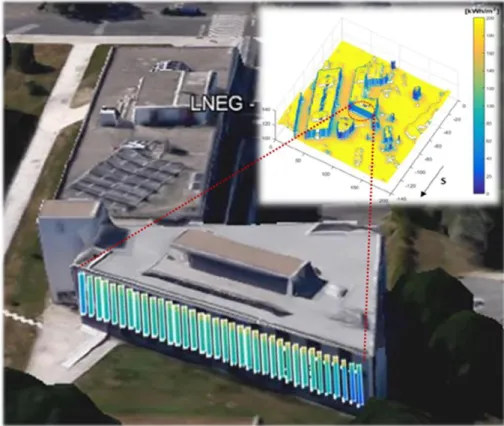
Carlos Rodrigues and Antonio Joyce from LNEG for providing the electricity production data from the Solar XXI PV façade used in the validation of the SOL model.

EDP Distribuição for providing the load demand data associated to the distribution power transformers in Lisbon.

MIT Portugal SES program coordinator in FCUL João Serra, for his support during the 1st_{year advanced}

course and in financial and travel matters, and MIT Portugal communications director Sílvia Castro, for sharing my humble achievements with the media.

Christoph Reinhart, for the stimulating lectures and discussions during my visit to the Sustainable Design Lab (MIT), and his team of inspirational, hardworking and kind individuals.

Gilles Desthieux and Claudio Carneiro, for sharing their experiences as senior researchers and for engaging in fruitful discussions during my visit to HEPIA.

MSc students with whom I explored dark waters and deepened my knowledge: André Cristóvão, Ana Barros, João Segadães, Inês Martinho, Sérgio Guimarães, Bernardo Tavares and Sofia Ganilha.

Ex- and current openspace colleagues: Mário Pó, Ivo Costa, Joana Baptista, Rodrigo Silva, Raquel Figueiredo, Pedro Nunes, Ângelo Casaleiro, Rita Montes, José Silva, Rita Almeida, Filipe Serra, David Pera. One does not simply forget all the funny moments, engaging discussions, absurd situations, outreach preparation, sweet pastry and tea time, outdoor lunches, adventures abroad,…

(6)

Aos que têm alimentado a minha criatividade musical e performativa, a minha imaginação, sem a qual tudo seria muito menos interessante: os Monolith Moon, o Grupo Coral Stravaganzza, o Gonçalo Antunes e os PSI.

Ao João e à Paula, pela partilha, a humildade, e por me guiarem no caminho do ashtanga yoga, a cola que une e me faz compreender tudo o resto.

À Daniela Fonte, pela amizade intemporal, pelo apoio constante aos meus projetos científicos e artísticos. Pelos bons momentos de gulodice!

À família emprestada, Pires e Gamito, junto dos quais o tempo parece parar. A boa vontade não se agradece, mas a minha gratidão pela amizade e pelas boas memórias é imensa.

Aos meus pais e irmão, pelo amor incondicional, por estarem sempre presentes nos bons e maus momentos e pelos valores que me têm transmitido ao longo da vida.

Ao Carlos, por tudo.

(7)

ABSTRACT

Consistent reductions in the costs of photovoltaic (PV) systems have prompted interest in applications with less-than-optimum inclinations and orientations. That is the case of building façades, with plenty of free area for the deployment of solar systems. Lower sun heights benefit vertical façades, whereas rooftops are favoured when the sun is near the zenith, therefore the PV potential in urban environments can increase twofold when the contribution from building façades is added to that of the rooftops. This complementarity between façades and rooftops is helpful for a better match between electricity demand and supply.

This thesis focuses on: i) the modelling of façade PV potential; ii) the optimization of façade PV yields; and iii) underlining the overall role that building façades will play in future solar cities.

Digital surface and solar radiation modelling methodologies were reviewed. Special focus is given to the 3D LiDAR-based model SOL and the CAD/plugin models DIVA and LadyBug. Model SOL was validated against measurements from the BIPV system in the façade of the Solar XXI building (Lisbon), and used to evaluate façade PV potential in different urban sites in Lisbon and Geneva. The plugins DIVA and LadyBug helped assessing the potential for PV glare from façade integrated photovoltaics in distinct urban blocks.

Technologies for PV integration in façades were also reviewed. Alternative façade designs, including louvers, geometric forms and balconies, were explored and optimized for the maximization of annual solar irradiation using DIVA. Partial shading impacts on rooftops and façades were addressed through SOL simulations and the interconnections between PV modules were optimized using a custom Multi-Objective Genetic Algorithm.

The contribution of PV façades to the solar potential of two dissimilar neighbourhoods in Lisbon was quantified using SOL, considering local electricity consumption. Cost-efficient rooftop/façade PV mixes are proposed based on combined payback times. Impacts of larger scale PV deployment on the spare capacity of power distribution transformers were studied through LadyBug and SolarAnalyst simulations. A new empirical solar factor was proposed to account for PV potential in future upgrade interventions. The combined effect of aggregating building demand, photovoltaic generation and storage on the self-consumption of PV and net load variance was analysed using irradiation results from DIVA, metered distribution transformer loads and custom optimization algorithms.

SOL is shown to be an accurate LiDAR-based model (nMBE ranging from around 7% to 51%, nMAE from 20% to 58% and nRMSE from 29% to 81%), being the isotropic diffuse radiation algorithm its current main limitation. In addition, building surface material properties should be regarded when handling façades, for both irradiance simulation and PV glare evaluation. The latter appears to be negligible in comparison to glare from typical glaze/mirror skins used in high-rises.

Irradiation levels in the more sunlit façades reach about 50-60% of the rooftop levels. Latitude biases the potential towards the vertical surfaces, which can be enhanced when the proportion of diffuse radiation is high. Façade PV potential can be increased in about 30% if horizontal folded louvers becomes a more common design and in another 6 to 24% if the interconnection of PV modules are optimized.

In 2030, a mix of PV systems featuring around 40% façade and 60% rooftop occupation is shown to comprehend a combined financial payback time of 10 years, if conventional module efficiencies reach 20%. This will trigger large-scale PV deployment that might overwhelm current grid assets and lead to electricity grid instability. This challenge can be resolved if the placement of PV modules is optimized to increase self-sufficiency while keeping low net load variance. Aggregated storage within solar

(8)

communities might help resolving the conflicting interests between prosumers and grid, although the former can achieve self-sufficiency levels above 50% with storage capacities as small as 0.25kWh/kWpv.

Business models ought to adapt in order to create conditions for both parts to share the added value of peak power reduction due to optimized solar façades.

(9)

RESUMO

As reduções continuas e consistentes no custo dos sistemas fotovoltaicos registadas nos últimos anos têm estimulado o interesse em aplicações com orientações e inclinação que não as ótimas. Este é o caso das fachadas dos edifícios, que possuem uma vasta área livre e disponível para a instalação de sistemas de energia solares. Do ponto de vista da geração de eletricidade via fotovoltaico, alturas solares menores são mais benéficas para as superfícies verticais nos edifícios, como as fachadas, enquanto que os telhados, horizontais ou inclinados, irão produzir mais quando o sol estiver mais próximo do zénite. Deste modo, o potencial solar fotovoltaico no meio urbano pode aumentar em duas vezes quando à produção pelos telhados se junta a contribuição das fachadas dos edifícios. Esta complementaridade entre fachadas e telhados permite uma maior facilidade de ajuste entre o perfil de consumo e o perfil de fornecimento de eletricidade nos edifícios e nas cidades.

A tese desenvolvida na presente dissertação foca-se, assim, em: i) explorar ferramentas para a modelação do potencial solar fotovoltaico nas fachadas dos edifícios; ii) testar formas alternativas de otimizar os ganhos de sistemas fotovoltaicos em fachada; e iii) salientar o papel fundamental que as fachadas solares irão desempenhar nas cidades do futuro.

Diversas metodologias para a construção de modelos digitais de superfície urbanos e para a simulação da radiação solar nesses contextos foram revistas. Atenção especial é dada ao modelo tridimensional SOL, baseado em dados LiDAR, e aos plug-ins DIVA e LadyBug, para o software CAD Rhinoceros 3D. O primeiro sofreu um processo de validação através da comparação com medidas de produção elétrica feitas no sistema fotovoltaico integrado na fachada do edifício Solar XXI, localizado no Lumiar, em Lisboa. Este modelo foi depois utilizado para avaliar o potencial fotovoltaico em várias zonas urbanas em Lisboa e também em Genebra, na Suíça. As outras duas ferramentas, baseadas do método

raytracing com as propriedades físicas dos materiais implementado em Radiance, serviram, numa

primeira fase, para avaliar potenciais impactos visuais nos espaços exteriores consequentes da reflexão da luz por módulos fotovoltaicos instalados em fachadas.

Tecnologias existentes no mercado e protótipos de produtos fotovoltaicos para fachadas foram igualmente revistos. Designs de elementos alternativos para fachadas, incluindo palas fixas horizontais e verticais e formas geométricas tridimensionais foram exploradas e as suas dimensões otimizadas para que a coleção anual de radiação solar fosse máxima. Foram também estudadas as dimensões otimizadas de varandas contendo painéis bifaciais sujeitos à radiação refletida por diferentes materiais nas envolventes. O plugin DIVA foi usado nestes estudos. No passo seguinte, averiguaram-se as consequências negativas do sombreamento parcial em sistemas fotovoltaicos em telhados e fachadas teste, através de simulações realizadas pelo modelo SOL. Um algoritmo genético multi-objectivo foi proposto como uma possível metodologia para alcançar uma solução com custo-benefício opimo para a localização dos módulos fotovoltaicos e como devem ser ligadas as strings sujeitos a sombreamento parcial.

A contribuição de fachadas fotovoltaicas para o potencial solar foi quantificada em duas localidades distintas em Lisboa usando simulações pelo modelo SOL, considerando o perfil de consumo de eletricidade no local. Várias percentagens de telhado/fachada com um bom compromisso entre produção e custos de investimento são propostas com base no tempo de retorno financeiro. Numa última fase, foram estudados os impactos adversos que uma penetração fotovoltaica a grande escala pode ter nos equipamentos da rede de distribuição elétrica, nomeadamente na capacidade de os transformadores locais receberem toda a eletricidade excedente produzida pelos sistemas fotovoltaicos. A ferramenta SolarAnalyst foi aqui utilizada para simular a irradiação nos telhados, enquanto que nas fachadas a irradiação foi obtida através do plugin LadyBug. Foi proposto um fator

(10)

solar empírico que seja incorporado nas metodologias de substituição de transformadores antigos ou no dimensionamento de novos equipamentos para zonas urbanas em construção. O efeito combinado da agregação dos consumos de eletricidade, da produção agregada de telhados e fachadas e do armazenamento agregado de vários edifícios no nível de autoconsumo foi analisado em detalhe. A variância de carga na rede elétrica foi também incluída no estudo dada a existência de dados reais de consumo a nível dos transformadores de dois bairros em Lisboa. Também aqui foi utilizado o plugin DIVA para simular a irradiação solar horária em todas as superfícies dos edifícios.

O modelo SOL mostrou-se razoavelmente exato, tendo em conta as limitações impostas pela natureza dos dados LiDAR. Foram alcançados Erros Viés Médios normalizados na ordem de 7% a 51%, Erros Absolutos Médios normalizados entre 20% e 58% e Raízes do Erro Quadrático Médio de 29% a 81%. A principal limitação da versão atual deste modelo deve-se ao algoritmo de radiação difusa ser isotrópico. Por outro lado, percebeu-se que as propriedades físicas dos materiais constituintes das superfícies dos edifícios devem ser levadas em conta quando se analisam as fachadas, tanto em termos da irradiação como no potencial de encadeamento visual. O ultimo, porém, aparenta ser pouco significativo em comparação com outros materiais típicos de construção como envidraçado e espelho, muito comuns em arranha-céus.

Os níveis de irradiação nas áreas mais iluminadas das fachadas podem alcançar até 50-60% dos níveis calculados para os telhados, nas cidades analisadas. Um viés positivo existe à medida que o aumento da latitude se traduz num maior potencial solar nas superfícies verticais face às horizontais ou pouco inclinadas. Este efeito é ligeiramente amplificado se as condições atmosféricas no local forem propicias à ocorrência de céus cobertos e, portanto, a fração de radiação difusa for elevada. Por outro lado, o potencial fotovoltaico nas fachadas pode aumentar também por meio do design alternativo que, contemplando módulos fotovoltaicos integrados em palas fixas horizontais, pode chegar aos 30%. Uma otimização do posicionamento dos módulos e das interligações em strings pode contribuir com mais 6% a 24% de ganhos (ou perdas evitadas) no sistema.

No ano 2030, se a eficiência dos módulos fotovoltaicos convencionais alcançar os 20%, será possível obter tempos de retorno financeiro do investimento na ordem dos 10 anos, se um misto de 40% da área nas fachadas e 60% da área dos telhados numa cidade for ocupado por sistemas solares. Nos anos seguintes, a manter-se essa tendência de redução de custos e aumento da eficiência, a introdução de sistemas fotovoltaicos a grande escala será impulsionada. Apesar de as fachadas permitirem alargar o período de produção e, portanto, um melhor ajuste da geração ao perfil de consumo local, a rede elétrica atual revela-se incapaz de suportar a injeção de produção excedente dos trilhados orientados a sul e da vasta área de fachada num cenário 100% penetração fotovoltaica, o que pode levar a instabilidade na rede. Este desafio pode ser resolvido recorrendo a uma otimização da localização de cada modulo fotovoltaico nas superfícies dos edifícios de modo a aumentar o autoconsumo e a minimizar a variância de carga na rede. Sistemas de armazenamento de eletricidade agregados ao nível de comunidades solares poderão aliviar o conflito de interesses entre prosumidores e a entidade reguladora da rede, apesar de ser possível aos primeiros obter níveis de autoconsumo acima dos 50% sem qualquer capacidade de armazenamento, ou alguma na ordem dos 0.25kWh/kWpv. Modelos de negócio alternativos terão que ser criados ou os atuais terão que se adaptar de maneira a serem criadas condições que permitam a ambas as partes partilhar do valor acrescentado consequente de um pico de potencia na rede reduzido graças às fachadas fotovoltaicas.

(11)

LIST OF FIGURES

Figure 1.1 – Spectral irradiance of: a 5900K blackbody, the sun light outside Earth’s atmosphere and at sea level (Valley, 1965). ... 28 Figure 2.1 – Steps and options involved in the assessment of solar potential at a certain location. ... 35 Figure 2.2 - Schematic representation of the radiation reaching a tilted surface by the sky anisotropic concept, including the anisotropy of the ground reflected component. It is important to note that the sky and horizon diffuse components may as well not be perfectly isotropic. (Adapted from Magarreiro et al., 2016). ... 38 Figure 2.3 – Variety of sky division strategies to calculate SVF (Marsh, 2011)... 40 Figure 2.4 – Example of an insolation analysis in the summer and winter as seen in Townscope (Teller and Azar, 2001). ... 44 Figure 2.5 – Distribution of daylight availability in an urban setting computed by SOLENE (Miguet, 2007). ... 45 Figure 2.6 - Global clear-sky solar irradiation for the month of January, as represented by v.sun (Hofierka and Zlocha, 2012). ... 46 Figure 2.7 – Comparison between the irradiation on the vertical plane and for an optimal inclination, modelled in (Esclapés et al., 2014). ... 46 Figure 2.8 - Irradiation analysis for multiple building façades and rooftops using SURFSUN3D (Liang et al., 2015). ... 47 Figure 2.9 - Mean solar irradiance collected by the second storey of each façade on the 10th_of

December at noon, obtained through the methods presented in (Carneiro et al., 2010). ... 47 Figure 2.10 - Annual global radiation over façades, roofs and ground as computed by SOL (Catita et al., 2014). ... 48 Figure 2.11 - Annual irradiation for a surface model with detailed rooftops (Jakubiec and Reinhart, 2013). ... 49 Figure 2.12 - SORAM simulation of global radiation distribution at heights of 0 m and 11.3 m (Erdélyi et al., 2014). ... 50 Figure 2.13 – Example of the 3D visualisation of the shortwave irradiance computed by SEBE model (Lindberg et al., 2015). ... 50 Figure 2.14 – Global radiation over the façades of a urban 3D model as presented by Ecotect (Ecotect, 2010). ... 51 Figure 2.15 – Implementation of rooftop solar PV using Skelion (Skelion, 2013). ... 52 Figure 2.16 – DIVA typical false colour visualization of irradiance results (Jakubiec and Reinhart, 2011). ... 52 Figure 2.17 – Example of sunlight hour analysis over a 3D model using LadyBug (Roudsari and Pak, 2013). ... 53 Figure 2.18 – Solar irradiation for the façade surfaces of a 3D building model as represented by Solar Analysis plug-in for Revit (Egger, 2016). ... 54 Figure 2.19 – Example of irradiance on a custom project and simulation of a rooftop PV system (PVsites, 2017). ... 54 Figure 2.20 - Annual solar irradiation [kWh/m2_{] estimated using CitySim (Mohajeri et al., 2016). ... 55}

Figure 2.21 - Radiation map simulated using SimStadt (Romero Rodríguez et al., 2017a). ... 56 Figure 2.22 - Direct irradiation over two city models for the 15th_{of June (left) and the 15}th_{of January}

(right) calculated using the methodology in (Bremer et al., 2016). ... 56 Figure 2.23 – Global horizontal radiation as presented by PVGIS database and its graphical user interface (JRC EC, 2014). ... 58 Figure 2.24 – PVWATTS user interface for rooftop PV systems costumization (NREL, 2017). ... 59

(14)

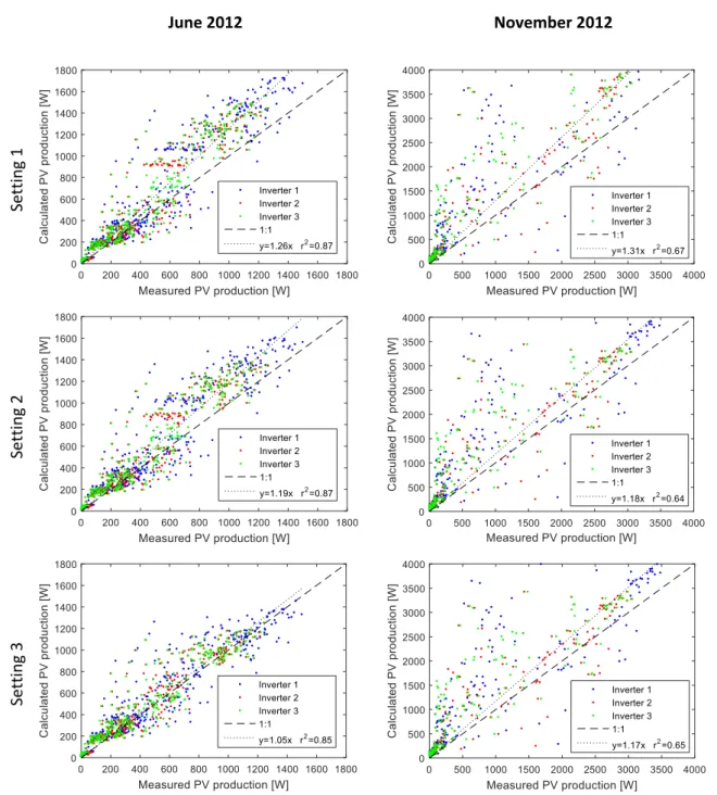
Figure 2.25 – User interface in Mapwell Solar Systems for assessing cost and revenue from a costumized PV rooftop (Mapdwell, 2017). ... 59 Figure 2.26 – Sunlight hour levels on rooftops as presented by Google Sunroof (Google, 2017). ... 60 Figure 3.1 – Incidence of direct sunlight in vertical façades and tilted rooftops in: a) morning/afternoon; and b) around noon. ... 65 Figure 3.2 - Location of the 13 shooting places in FCUL campus. Points 1, 3 and 4 belong to a façade (Freitas et al., 2016a). ... 66 Figure 3.3 - Fisheye photographs taken in the 13 shooting places in FCUL campus (Freitas et al., 2016a). ... 67 Figure 3.4 - Four sky vaults studied: 145, 290, 400 and 1081 divisions (Freitas et al., 2016a). ... 67 Figure 3.5 - SVF values obtained with 4 different sky vaults in comparison with the fisheye photographs processed with the annulus and the pixel methods (Freitas et al., 2016a). ... 68 Figure 3.6 - Façade integrated PV system in the Solar XXI building, in LNEG, Lisbon (Freitas and Brito, 2017a). ... 69 Figure 3.7 - Distribution of modules in the façade and interconnections of the strings to the respective inverter (Rodrigues, 2008), and the location of the radiation sensor (red dot). ... 69 Figure 3.8 – Global vertical (red), global horizontal (blue) and diffuse horizontal (black) irradiances for the months of June (top) and November (bottom) of 2012. ... 70 Figure 3.9 – Scatter plots of the recorded module temperature against ambient temperature, and respective linear regression, for the months of June (left) and November (right) of 2012. ... 70 Figure 3.10 - Cumulative solar irradiation estimated for the month of June 2012 (inset) and the façade points superimposed over a Google Earth view of the building (Freitas and Brito, 2017a). ... 71 Figure 3.11 – Global vertical irradiation measured by the sensor against results produced by SOL in an approximate position, for June (left) and November (right). ... 71 Figure 3.12 - Comparison between the calculated and measured PV production by inverter, for June (left) and November (right) of 2012: Setting 1 (top); Setting 2 (middle); and Setting 3 (bottom). (Freitas and Brito, 2017a) ... 74 Figure 3.13 – Boxplot representation of the hourly relative deviation in June (top) and November (bottom) of 2012, for the 3 Inverters (columns) and through the 3 Methods (rows). (The tops and bottoms of each "box" are the 25th_{and 75}th_{percentiles, the red line in the middle of each box is the}

median, the black lines extending above and below each box are the extreme values and the red crosses are the outliers.) (Freitas and Brito, 2017a) ... 75 Figure 3.14 – Bird’s eye view and street view of the 4 studied areas: A (38.748630, -9.136996), B (38.738929, -9.144399) and C (38.756064, -9.156481) in Lisbon, Portugal; and D (46.229499, 6.079182) in Geneva, Switzerland, retrieved from Google Maps. ... 77 Figure 3.15- Yearly solar irradiation in the areas A, B, C and D. The false colour scale highlights the places with lower (blue) and higher (red) solar potential. The vertical dimensions are different in the 4 maps: tallest buildings reach around 60m in area A, 50m in area B, 40m in area C and 30m in area D (Freitas et al., 2016b). ... 78 Figure 3.16- Annual solar potential histogram. Dashed lines refer to roofs and solid lines to façades with different colours according to South, East, West and North orientation (i.e. points with azimuth inside the intervals [45°, 135°[, [135°, 225°[, [225°, 315°[ e [315°, 45°[ where 0° denotes North) (Freitas et al., 2016b). ... 79 Figure 3.17 – Rooftop meshes over the building geometries in Rhinoceros 3D viewport (left) and a detail on DIVA-for-Grasshopper Radiation Map components (right). ... 81 Figure 3.18 - Input features for estimating the irradiation using the footprint method (top), the LiDAR method (middle) and the sketch method (bottom), for Blocks 1 and 2. Note that only the buildings with red rooftops are part of the studied blocks. ... 82

(15)

Figure 3.19 - Annual solar irradiation for Blocks 1 and 2 using the footprint method (top), the LiDAR method (middle) and the sketch method (bottom). ... 83 Figure 3.20 - Hourly difference relatively to the Sketch method between solar irradiation on rooftops estimated using the Footprint method and the LiDAR method, for Block 1 and 2. Negative values mean overestimation. (The tops and bottoms of each "box" are the 25th_{and 75}th_{percentiles, the red line in}

the middle of each box is the median, the black lines extending above and below each box are the extreme values and the red crosses are the outliers.) ... 84 Figure 3.21 – Case-study building, located in Lisbon, with high reflective glass façades: bird’s eye view (left) and reflection detail (right). Retrieved from Google Earth at 38.7445618, -9.159805. ... 85 Figure 3.22 – Digital surface model of the target building (circled) and its surroundings (green represents grass, blue the nearby buildings with blue façades and red are mirror surfaces). ... 86 Figure 3.23 – Example of the LadyBug component “Sunpath” with solar path diagram and hourly sun positions for December (top) and component “Bounce from surface” with respective sun rays (bottom). ... 86 Figure 3.24 – Cumulative density of reflected rays that intersect the ground in the four typical days (left) and camera positions (right). ... 87 Figure 3.25 – RGB values for the different shades in the false colour bands of glare images. ... 88 Figure 3.26 – Example of a false colour luminance image for Camera 3, for the 20th_{of June at 10h (left)}

and respective mask excluding all but the target building façades (right). ... 89 Figure 3.27 – Cumulative frequency of luminance classes per façade material. ... 89 Figure 3.28 – PV and mirror luminance images for cameras 1, 2 and 3 in the summer and winter solstices and autumn equinox, for the morning, midday and afternoon periods. ... 90 Figure 4.1 – Examples of distributed in-house electricity generation with a synthesis of PV and conventional construction materials. (ViaSolis, 2017). ... 93 Figure 4.2 –Back ventilated glass PV rainscreen system, Dresden, Germany (Bendheim, 2010). ... 94 Figure 4.3 – PV curtain wall in Greenstone Government of Canada Building (Manasc Isaac, 2005). .. 94 Figure 4.4 – Double skin PV façade with 0.8m of air gap in the Norwegian University of Science and Technology, Trondheim (Horisun, 2000). ... 95 Figure 4.5 – Solar PV window tests at FLEXLAB, Solaria BIPV (Solaria, 2016). ... 95 Figure 4.6 – Solar sunshades at a museum in Canada (Taste of Nova Scotia, 2015) (left) and sliding window shutters with frameless PV modules in a German house (Manz AG, 2017) (right). ... 96 Figure 4.7 – Triangular c-Si modules installed in one façade of the International Centre for Design, in Saint-Etienne (Vincent Fillon, 2009). ... 97 Figure 4.8 – Thin film PV products integrated on building façades: a-Si modules (EcoFloLife, 2017) (left) and CIGS (Global Solar Inc., 2017) (right). ... 97 Figure 4.9 – Air-based PV-thermal system in a building façade in Montreal (Athienitis et al., 2011). . 98 Figure 4.10 – Façade integrated PV-thermal prototype in Hong Kong for water pre-heating (Chow et al., 2007). ... 98 Figure 4.11 - Bifacial wall at Green Dot Animo School (left) and a façade bifacial prototype with white reflector sheet (Hezel, 2003) (right). ... 98 Figure 4.12 – Red glass-glass PV modules in the balustrade of Villa Circuitus, in Sweden (Wesslund and Kreutzer, 2015) (top, left); green PV sunscreens, in London (LOF Solar Corporation, 2014) (top, right); green screen printing on front glass of façade integrated c-Si modules, in Oslo (Issol, 2015) (bottom, left); vertical white PV modules (Solaxess, 2017) (bottom, right). ... 99 Figure 4.13 – Disguised PV modules for façade application (Slooff and et al., 2017) (left) and coloured PV façades in a school in Copenhagen (John Fitzgerald Weaver, 2017) (right). ... 100 Figure 4.14 –Glass with OPV design for vertical applications (OPVIUS, 2017) (left) and tracking DSSC sunshades in the façade of Swiss-Tech Convention Centre in Lausanne (Solaronix, 2014) (right). ... 100

(16)

Figure 4.15 – Example of semi-transparent PV canopy (left) and a solar OPV window made from a mixture of carbon, hydrogen, oxygen and nitrogen (Solar Window Technologies, 2017) (right). ... 101 Figure 4.16 – Prototype of a PVCC in: a) opaque state, under 1 sun; and b) bleached state, under 0 sun (Favoino et al., 2016). ... 101 Figure 4.17 – Transparent luminescent solar concentrator with PV cells attached to the edges (Physee, 2017) (left) and external PV louvers for Windows (SolarGaps Inc., 2017) (right). ... 101 Figure 4.18 – Vertical (Chemisana and Rosell, 2011) (top) and horizontal (Valckenborg and et al., 2016) (bottom) reflective solar concentrators. ... 102 Figure 4.19 – Examples of stationary 2D parabolic concentrators for wall integration: (Mallick and Eames, 2007) (top) and (Brogren et al., 2003) (bottom). ... 103 Figure 4.20 – Total internal reflection 3D solar concentrators (Baig et al., 2015) (left) and (Abu-Bakar et al., 2016) (right). ... 104 Figure 4.21 - Flat CPV module with Fresnel lenses for façade integration (Bunthof et al., 2016) (top) and concentrating spherical glass lens with dual axis tracking and triple junction PV cells (Caula, 2012) (bottom). ... 105 Figure 4.22 - Integrated Concentrating Solar Façade prototypes for building-integrated PV (CASE, 2016). ... 105 Figure 4.23 – Underlying principle behind LSC (left); LSC installed in vertical noise barriers (Slooff and et al., 2016) (middle); and cylindrical LSC with near-infrared quantum dots (Inman et al., 2011) (right). ... 106 Figure 4.24 – Transition from fully transparent to translucent state of the reflective concentrating PV smart window prototype (Connelly et al., 2016). ... 107 Figure 4.25 - Trackless holographic concentrating PV modules for buildings and urban furniture (Rodríguez San Segundo and et al, 2016) and the Holographic Planar Concentrator by Prism Solar Technologies, Inc. ... 107 Figure 4.26 – Solar thermal collectors integrated in façade elements (Sunaitec, 2014). ... 108 Figure 4.27 – Electricity generating dye-sensitized concrete prototypes with colour and bending properties (Building Art Invention, 2017). ... 108 Figure 4.28 – Examples of functional and unconventional façade elements in: Belgium (IBA Technics, 2015) (1), Germany (Stylepark, 2016) (2), Korea (American Institute of Architects, 2015) (3), France (Vergne, 2011) (4), China (Frearson, 2013) (5) and Portugal (CML, 2017) (6). Geometries in pictures 5 and 6 are non-PV. ... 111 Figure 4.29 - Studied façade layouts: flat walls (base), horizontal and vertical rotated/folded louvers (2-4), wall ellipsoids (5) and wall pyramids (6). PV surfaces are coloured in blue. ... 111 Figure 4.30 - Overall workflow view of the modelling tools (top) and a detail on the DIVA 3.0 solar irradiation components used (bottom). ... 112 Figure 4.31 – Overview of the evolutionary optimization through the component Galapagos. In the leftmost side, the component is connected to the sliders that define the tilt angle of horizontal rotated louvers. ... 112 Figure 4.32 – Annual irradiation for the east- (top), south- (middle) and west-facing (bottom) vertical façades in Lisbon (left column) and Oslo (right column). The value in the lower left corner of each image corresponds to the total annual solar irradiation [kWh/year]. ... 113 Figure 4.33 - Optimal E+S+W rotated louvers, for Lisbon (left column) and Oslo (right column). ... 114 Figure 4.34 – Optimal E+S+W folded louvers, for Lisbon (left column) and Oslo (right column). ... 115 Figure 4.35 - Optimal E+S+W wall ellipsoids and hexagonal pyramids, for Lisbon (left column) and Oslo (right column). ... 116 Figure 4.36 – Estimated annual electricity production from the different façades for Lisbon (yellow) and Oslo (grey): layout total (top) and density per PV occupied area (bottom). (100% means 10.0

(17)

MWh/year and 0.11 MWh/year/m2

PV, for Lisbon, and 5.8 MWh/year and 0.06 MWh/year/m2PV, for

Oslo) (Freitas and Brito, 2015). ... 117 Figure 4.37 – Horizontal (left) and optimal (right) SE+SW rotated louvers, for Lisbon (Freitas and Brito, 2015). ... 117 Figure 4.38 – Yearly irradiation for optimal louver tilt under conservative partial shading, for east-, southeast-, south-, southwest- and west-facing façades (Freitas and Brito, 2015). ... 118 Figure 4.39 – Examples of balcony integration of PV in Finland (Solpros, 2003) (top left), Germany (Donahue, 2017) (top right), Austria (LOF Solar Corporation, 2010) (bottom left) and France (SADEV, 2015) (bottom right). ... 119 Figure 4.40 – Render view of archetype with PV modules on the balcony railings (left) and detail of the elements considered in the parametric modelling (right) (Freitas and Brito, 2016). ... 120 Figure 4.41 - Lisbon: annual solar irradiation in the front and back railing surfaces for the E+S+W+N (left) and NE+SE+SW+NW (right) configurations (Freitas and Brito, 2016). ... 121 Figure 4.42 - Balcony depths, widths and offsets [m] obtained in the optimization process (Freitas and Brito, 2016). ... 121 Figure 4.43 - Estimated front and rear PV generation density [kWh/m2/year] for each orientation and location with optimized balcony dimensions and materials (Freitas and Brito, 2016). ... 122 Figure 4.44 - Decrease in PV generation from the optimized dimensions and materials to the scenario with poor reflective materials. ... 123 Figure 4.45 - Detail of the simulation with partial-shadow cast by a person standing in a south facing balcony, in Lisbon (Freitas and Brito, 2016). ... 123 Figure 5.1 – Main scheme of the genetic algorithm (Freitas et al., 2015a). ... 128 Figure 5.2 – Example of a chromosome and its encoding strategy. The different colours highlight different PV strings (Freitas et al., 2015a). ... 129 Figure 5.3 - Rooftop 1 (yellow circle) and surroundings coloured according to the height. The ground height of 100m corresponds to the average of the city of Lisbon (Freitas et al., 2015a). ... 134 Figure 5.4 - Orthogonal view of the hourly irradiation [Wh/m2_{] in rooftop 1, for a winter (top row) and}

a summer (bottom row) day. (Freitas et al., 2015a). ... 135 Figure 5.5 – Photograph of an afternoon shadow cast on façade 1 (portion signed in yellow). ... 135 Figure 5.6 – Orthogonal view of the hourly irradiation [Wh/m2_{] in façade 1, for a winter (top row) and}

a summer (bottom row) day. White denotes excluded positions (Freitas et al., 2015a). ... 135 Figure 5.7 - Bird’s eye perspective to rooftop 2 (left) and street view of façade 2 (right), retrieved from Google Earth at approximately 38.7398959, -9.1463554. ... 136 Figure 5.8 – Yearly total PV production per string of a typical line wise (left) and a column wise (right) distribution of PV strings, for rooftop 1. Note the different colour scale values in the two graphs (Freitas et al., 2015a). ... 136 Figure 5.9 – Rooftop 1 layout with lowest cost of electricity achieved in the 70th_{(left) and 250}th_(right)

generations (Freitas et al., 2015a). ... 137 Figure 5.10 – Charts with the overview of the relevant Cost and Energy variables during the optimization process, for rooftop 1 (Freitas et al., 2015a). ... 137 Figure 5.11 - Comparison between the Pareto fronts from the initial (left) and 250th_{(right) generations,}

for rooftop 1. The arrow points the individual with minimum cost of energy [€/kWh] (i.e. 0.063€/kWh and 2240kWh/year) and the yellow circles mark the location of the conventional solutions presented in Figure 5.8 (i.e. 0.077€/kWh and 2173kWh/year; 0.080€/kWh and 2305kWh/year). Background shading marks different levels of €/kWh (Freitas et al., 2015a). ... 138 Figure 5.12 – Yearly total PV production per string of a typical column wise distribution of PV strings, for façade 1. White areas mean unavailable positions for module deployment (Freitas et al., 2015a). ... 138

(18)

Figure 5.13 - Façade 1 layout with lowest cost of electricity achieved in the initial (left) and 400th_(right)

generations. Zeros (darkest blue) denote areas without deployment of modules and white means unavailable positions (Freitas et al., 2015a). ... 139 Figure 5.14 – Comparison between the Pareto fronts from the initial (left) and 400th_{(right) generations,}

for façade 1. The arrow points the individual with minimum cost of energy [€/kWh] in (i.e. 0.209€/kWh and 997kWh/year) and the yellow circle marks the location of the conventional solution presented in Figure 5.12 (i.e. 0.221€/kWh and 1215kWh/year). Background shading marks different levels of €/kWh (Freitas et al., 2015a). ... 139 Figure 5.15 - Charts with the overview of the relevant Cost and Energy variables during the optimization process, for façade 1 (Freitas et al., 2015a). ... 140 Figure 5.16 - Yearly total PV production per string of the optimized distribution of strings (left) and the micro-inverter scenario (right), for the rooftop 2. Zeros (darkest blue) denote areas without deployment of modules. Note the different colour scale values in the two graphs (Freitas et al., 2015b). ... 140 Figure 5.17 - Comparison between the Pareto fronts from the initial (left) and 400th_{(right) generations,}

for façade 2. The arrow points the individual with minimum cost of energy [€/kWh] (i.e. 0.22 €/kW h and 731 kW h/year) and the green triangle marks the location of the micro-inverter scenario (Freitas et al., 2015b). ... 141 Figure 5.18 - Yearly total PV production per string of the optimized distribution of strings (left) and the micro-inverter scenario (right), for the façade 2. Zeros (darkest blue) denote areas without deployment of modules and white means unavailable positions. Note the different colour scale values in the two graphs (Freitas et al., 2015b). ... 141 Figure 5.19 - Comparison between the Pareto fronts from the initial (left) and 400th_{(right) generations.}

The arrow points the individual with minimum cost of energy [€/kWh] (i.e. 0.30 €/kW h and 711 kW h/year) and the green triangle marks the location of the micro-inverter scenario (Freitas et al., 2015b). ... 142 Figure 6.1 - Annual electricity demand per building, for Area A (left) and Area B (right) (Brito et al., 2017). ... 148 Figure 6.2 - Monthly PV potential (roofs: dark brown column; façades: lighter brown columns according to 4 different classes: above 900kWh/m2_{/year, between 700 and 900, between 500 and 700, and}

below 500kWh/m2_{/year) and electricity demand (blue solid line: non-baseload monthly electricity}

demand; blue dashed line: monthly total electricity demand) for Area A (left) and Area B (right) (Brito et al., 2017). ... 148 Figure 6.3 - Solar radiation for Area A (left) and Area B (right) at 12:00 LST on December 21st_{(top) and}

09:00 LST on June 21st_{(bottom) (Brito et al., 2017). ... 151}

Figure 6.4 - Hourly electricity demand (dark blue line) and photovoltaic potential of roofs (black dashed line), all façades (black solid line), south façades (orange), east façades (yellow), west façades (green), north façades (light blue) and roofs and façades (red), for Area A (left) and Area B (right) for a winter day (top) and a summer day (bottom) (Brito et al., 2017). ... 152 Figure 7.1 - Delimitation of Alvalade within Lisbon (blue area), part of Area A (orange dashed line), location of the transformers (red dots) and respective DSM of the area (Freitas et al., 2017a). ... 156 Figure 7.2 - Thiessen polygons depicting the influence zones of all transformers (top) and transformer power capacities [kVA] (bottom) (Freitas et al., 2017a). ... 157 Figure 7.3 - 3D model of the buildings inside the transformer influence zones and the number of residents per building (Freitas et al., 2017a). ... 158 Figure 7.4 - Seasonal reference electricity loads for single dwellings (Freitas et al., 2017a). ... 159 Figure 7.5 - Aggregated hourly electricity load and PV production (top) and transformers spare power (bottom), for the 21st_{of March, June, September and December, in the rooftops only (left) and}

(19)

Figure 7.6 - 𝑃𝐺𝐴𝑃 at each transformer influence zone considering rooftop PV generation using the Peak power method (A) and Irradiance method (B). Negative values/coloured zones indicate failure at the respective transformer (Freitas et al., 2017a). ... 161 Figure 7.7 - Absolute difference between the Peak power method and the Irradiance method (A) and difference relative to the respective transformer capacity (B). The grey shadows in the background represent the building footprints (Freitas et al., 2017a). ... 162 Figure 7.8 - 𝑃𝐺𝐴𝑃 at each transformer influence zone considering rooftop and façade PV generation using the Peak power method (A) and the Irradiance method (B). Negative values indicate failure at the respective transformer (Freitas et al., 2017a). ... 163 Figure 7.9 - Absolute difference between the Irradiance method and the Peak power method (A) and difference relative to the respective transformer capacity (B) considering building PV façades. The grey shadows in the background represent the building footprints (Freitas et al., 2017a). ... 164 Figure 7.10 - Boxplots representing the distribution of the maximum excess power demand/injected, as a percentage of the transformers capacity, for different storage capacities in all hours of the typical days analysed. (The tops and bottoms of each "box" are the 25th_{and 75}th_{percentiles, the red line in}

the middle of each box is the median, the green dots are the average, the black lines extending above and below each box are the extreme values and the red crosses are the outliers.) (Freitas et al., 2017b). ... 165 Figure 8.1 - Location of the project site (38°46'05" N, 9°05'38" W), urban context inside the project site boundary (top) and case-study Blocks 1 and 2 (bottom) (Freitas et al., 2018). ... 170 Figure 8.2 - Aggregated electricity consumption for Blocks 1 (left) and 2 (right): frequency of days with given demand normalized by total floor area (respectively 21242 m2_{and 17240 m}2_{) (Freitas et al.,}

2018). ... 171 Figure 8.3 - Frequency of average surface irradiation levels in Block 1: tilted rooftop (total of 1875 surfaces), façade (total of 4114 surfaces) and horizontal rooftop (total of 3600 surfaces) (Freitas et al., 2018). ... 172 Figure 8.4 - Frequency of average surface irradiation levels in Block 2: tilted rooftop (total of 1832 surfaces), façade (total of 1161 surfaces) and horizontal rooftop (total of 10 surfaces) (Freitas et al., 2018). ... 172 Figure 8.5 - Total hourly estimated electricity production from rooftops (blue), façades (green), rooftops and façades (black) and measured electricity demand (red), for Blocks 1 and 2, for one year. ... 173 Figure 8.6 - Histogram of the hourly net load variance over the period of 1 year, for Blocks 1 and 2. ... 176 Figure 8.7 - Example of the semi-random number generation in the encoding step of the optimization of the PV placement routine. (H stands for horizontal). ... 177 Figure 8.8 - Results from Scenario A-opt for Block 1 (left) and 2 (right): first (red) and second (blue) pareto fronts from the last generation. The cross marks the optimal solution. (Freitas et al., 2018) 179 Figure 8.9 - Optimum distribution of PV area on rooftops and façades for Scenario A-opt (no batteries). yy-axis shows total area available (bordered bar) and used for PV (coloured bar) as a fraction of total building area, for each orientation. Results for Block 1 (left) and Block 2 (right), rooftops (up) and façades (bottom). H stands for horizontal rooftop surfaces. (Freitas et al., 2018) ... 180 Figure 8.10 - Scenario A2 for Block 1 (left) and Block 2 (right): percentage of occupancy by PV modules of the azimuth bins available in rooftop and façade surfaces. ... 181 Figure 8.11 - Optimum distribution of PV area on rooftops and façades for Scenario B-opt (orange and light blue) and B-bau (red and dark blue), for Block 1 (left) and Block 2 (right), from lower (top) to higher storage capacity (bottom). yy-axis shows area used for PV as a fraction of total building area, for each orientation. The corresponding optimal PV peak power is given. Note that the percentages in

(20)

Figure 8.12 - Optimum distribution of PV area on rooftops and façades for Scenario C-opt (light green and light yellow) and C-bau (dark green and dark yellow), for Block 1 (left) and Block 2 (right), from lower (top) to higher storage capacity (bottom). yy-axis shows area used for PV as a fraction of total building area, for each orientation. The corresponding total PV peak power is given. Note that the percentages in the axis limits are different for the 2 blocks. (Freitas et al., 2018) ... 183 Figure 8.13 - Overall results for RMSDNLV, SS, SC and PPVS as a function of storage capacity, for

Scenarios B-opt (blue solid line), B-bau (blue dashed line), C-opt (orange solid line) and C-bau (orange dashed line). (Freitas et al., 2018)... 185

(21)

LIST OF TABLES

Table 1.1 – Research questions distribution by Chapters... 31 Table 3.1 – Normalized Mean Bias Error (nMBE), normalized Mean Absolute Error (nMAE) and normalized Root Mean Squared Error (nRMSE) by Inverter, for June and November of 2012, for Settings 1, 2 and 3. (Freitas and Brito, 2017a) ... 76 Table 3.2 – Contribution from rooftops and façades to the solar potential of the studied areas. Shaded values correspond to points with irradiation > 900kWh/m2_{/year. ... 79}

Table 3.3 – Relevant visual properties of the different material functions used. ... 87 Table 4.1 – Summary of reviewed PV technologies for building façade applications. ... 109 Table 4.2 – Optimized parameters for E+S+W horizontal and vertical folded louvers in Lisbon and Oslo. Positive/negative angle means to the right/left from the normal plane and ascending/descending. ... 115 Table 4.3 - Optimized parameters for E+S+W wall ellipsoids and hexagonal pyramids in Lisbon and Oslo. Positive/negative angle means to the right/left from the normal plane and ascending/descending. ... 116 Table 4.4 - Materials assigned to the optimized balcony designs (Freitas and Brito, 2016). ... 120 Table 5.1 – Typical pc-Si module parameters. ... 130 Table 5.2 - List of properties of 12 inverters and 1 micro-inverter. Prices retrieved between December 2014 and August 2015 from (Wholesale Solar, 2015)(CCL Componentes, 2014)(Energy Matters, 2014)(MG Solar, 2014). ... 132 Table 5.3 – Parameter specifications for the GA used in the rooftop and façade case-studies. ... 133 Table 5.4 – Yields and Costs obtained for the 4 case-studies in conventional columnwise, micro-inverter and optimized arrangements. ... 142 Table 6.1 - Annual energy demand and solar electricity production for the different system classes represented in Figure 6.2. ... 149 Table 6.2 - Financial payback time of investment for an average rooftop system and the threshold of the different façade classes. ... 150 Table 6.3 – Mix of roof and façade PV systems for different combined payback time periods. ... 150 Table 8.1 – Elementary battery characteristics. ... 174 Table 8.2 – Type of PV optimization and storage strategy in the considered scenarios (“bau” and “opt” stand for “business as usual” and “optimal” respectively). ... 177 Table 8.3 – Annual PV generation and load demand [MWh/year], and decision parameter values for scenarios A-bau and A-opt for Block 1 and 2. ... 181 Table 8.4 – Maximum absolute peak power in the electricity grid [kW], for Block 1 and 2. Bold highlights the 3 lowest peak power achieved for each Block. ... 187

(22)

(23)

NOMENCLATURE AND ABBREVIATIONS

Parameter/index Description

3DCM 3D city model

𝐴_{𝑏𝑢𝑖𝑙𝑑} [m2_] _{Total available area on all roof and façade surfaces}

𝐴_{𝑓𝑜𝑜𝑡} [m2_] _{Total building footprints area}

𝐴𝑓 [m2] Total installed PV area in the façade

𝐴_𝑟 [m2_] _{Total installed PV area in the rooftop}

𝐴_𝑠 [m2_] _{Area of surface 𝑠}

AC Alternating current

𝐴𝐿 [-] Losses due to angle of incidence ALS Aerial laser scanning

AVF Anisotropic view factor

𝑎_𝑟 [-] Empirical angular losses coefficient a-Si Amorphous silicon

𝐵𝑏𝑎𝑡 [kWh/kWpv] Storage capacity

𝐵_𝑒𝑥𝑝 [kWh] Electricity stored in the battery that was exported to the grid 𝐵_𝑠𝑐 [kWh] Electricity stored in the batteries that supplies for the loads 𝐵𝑠𝑜𝑐,𝑓 [kWh] Ending of cycle battery energy state of charge

𝐵_{𝑠𝑜𝑐,𝑖} [kWh] Beginning of cycle battery energy state of charge BIM Building Information Modelling

BAPV Building applied photovoltaics BIPV Building integrated photovoltaics 𝑏 [-] Block/building index

𝐶0 [€] Initial investment cost

𝐶𝑏𝑎𝑡 [€/kWh] Unitary cost of the battery

𝐶_{𝑑𝑖𝑣𝑒𝑟𝑠𝑖𝑡𝑦} [-] Simultaneity coefficient for consumption 𝐶𝑖 [€] Inverter cost

𝐶𝑚 [€/m2] Cost of conventional c-Si PV module

𝐶_𝑜𝑚 [€] Operation and maintenance costs 𝐶𝑝𝑣,𝑓 [€] Cost of the PV installation for the façade

𝐶𝑝𝑣,𝑟 [€] Cost of the PV installation for the rooftop

𝐶_{𝑟𝑎𝑡𝑒} [kW/kWh] Charging rate relative to maximum battery capacity 𝐶𝑟𝑒𝑝 [€] Replacement costs of the storage

𝐶𝑠 [€/m] PV string wiring cost

𝐶_{𝑠𝑦𝑠𝑡} [€] PV system investment cost 𝐶𝑦 [€] Cash flow in year 𝑦

CAD Computer-aided design CFD Computational fluid dynamics

CIE International Commission on Illumination CIGS Copper indium gallium (di)selenide CPV Concentrating photovoltaics c-Si Crystalline silicon

𝑑𝑔 [%/year] Degradation rate for PV 𝐷𝑖𝑟_{ℎ𝑜𝑟𝑖𝑧} [kWh/m2_{] Direct horizontal irradiation}

𝐷𝑖𝑟𝑛𝑜𝑟𝑚 [kWh/m2] Direct normal irradiation

(24)

𝐷𝑖𝑓𝑣𝑒𝑟𝑡 [kWh/m2] Diffuse vertical irradiation

DC Direct current

DIVA Design Iterate Validate Adapt DSM Digital surface model

DSSC Dye-sensitized solar cells DTF Diffuse tilt factor DUM Digital urban model 𝐸𝑑𝑒𝑚 [kWh] Electricity demand

𝐸_𝑖𝑚𝑝 [kWh] Electricity purchased from the grid 𝐸_{𝑠𝑦𝑠𝑡} [kWh/year] PV System anual electricity yield 𝑒𝑝 [€/kWh] Grid single tariff

𝑒_𝑠 [€/kWh] Retail electricity market prices

𝐹_𝑑𝑖𝑓[-] Transposition factor for diffuse irradiation

𝐹𝑟𝑒𝑓 [-] Transposition factor for ground reflected irradiation

𝐹_𝑃𝑉 [-] Solar factor for transformer sizing

𝐹𝑠𝑎𝑓𝑒𝑡𝑦 [-] Safety margin for power transformer capacity

FCUL Faculdade de Ciências, Universidade de Lisboa 𝐺_{ℎ𝑜𝑟𝑖𝑧} [kWh/m2_] _{Global horizontal irradiation}

𝐺𝑟𝑒𝑓 [kWh/m2] Reference global irradiation

𝐺_{𝑡𝑖𝑙𝑡𝑒𝑑} [kWh/m2_] _{Global irradiation in the tilted plane}

𝐺_{𝑣𝑒𝑟𝑡} [kWh/m2_] _{Global vertical irradiation}

GA Genetic algorithm

GIS Geographic information system GUI Graphical user interface

𝑔ℎ𝑜𝑟𝑖𝑧 [-] Normalized ratio between façade and horizontal rooftop electricity production

𝑔𝑜𝑝𝑡𝑖𝑚 [-] Normalized ratio between façade and optimal rooftop electricity production

ℎ [h] Hourly time step index H [h] Total number of hours

HPC Holographic planar concentrator 𝑖 [-] Inverter index

𝑖𝑛𝑓 [%] Inflation rate 𝑘𝐷 [-] Diffuse fraction

𝐿 [years] System lifetime 𝐿_𝑏𝑎𝑡[years] Battery lifespan

LiDAR Light detection and ranging LoD Level of detail

LSC Luminescent solar concentrator 𝐿𝑐 [m] Length of PV string wiring

𝑚 [-] PV module index 𝑀𝐴𝐸 Mean absolute error

𝑀𝐵𝐸 Mean bias error

MLS Mobile laser scanning

MOGA Multi objective genetic algorithm 𝑁_𝑏 [-] Total number of surfaces in Block 𝑏 NLV Net load variance

𝑁𝑂𝐶𝑇 [°C] Nominal operating cell temperature 𝑛_𝑏𝑎𝑡 [-] Number of batteries

nMAE Normalized mean absolute error nMBE Normalized mean bias error

(25)

nRMSD Normalized root mean squared deviation nZEB Net zero energy building

OGC Open geospatial consortium OPV Organic photovoltaics O&M Operation and maintenance 𝑃_{𝑐𝑜𝑛𝑡𝑟𝑎𝑐𝑡} [kW] Customer contracted power 𝑃_{𝑑𝑒𝑚𝑎𝑛𝑑} [kW] Local aggregated power demand 𝑃𝐺𝐴𝑃 [kW] Transformer spare power

𝑃_{𝑜𝑣𝑒𝑟} [kW] Transformer oversized power capacity 𝑃_𝑃𝑇 [kVA] Nominal power transformer capacity 𝑃𝑟𝑒𝑓 [W/m2] Nominal PV module power

𝑃_{𝑠𝑡𝑜𝑟𝑎𝑔𝑒} [kW/kWp] Local aggregated storage capacity

PT Power transformer

PV Photovoltaic

𝑃𝑉 [kWh] PV generated electricity

𝑃𝑉_𝑖 [kWh] PV electricity yields by inverter 𝑖 𝑃𝑉𝑚 [kWh] PV generated electricity by module 𝑚

𝑃𝑉_𝑏𝑎𝑡 [kWh] PV produced electricity that charges the storage bank 𝑃𝑉_𝑒𝑥𝑝 [kWh] PV produced electricity that was exported to the grid 𝑃𝑉𝑠𝑐 [kWh] Self-consumed PV generated electricity

PVCC Photovoltachromic cells 𝑝_𝑃𝑉 [kW/m2_] _{PV peak power density}

p-Si Polycrystalline silicon

𝑅𝑀𝑆𝐷 Root mean squared deviation 𝑟 [%] Opportunity cost of capital 𝑟𝑎𝑚𝑝 [kW/h] Hourly ramp rate

𝑆 [-] PV string index

SC [%] Self-consumption rate

𝑆𝑂𝐶_𝑚𝑎𝑥[%] Maximum state of charge relatively to the nominal battery capacity 𝑆𝑂𝐶𝑚𝑖𝑛 [%] Minimum state of charge relatively to the nominal battery capacity

SOL Solar out of LiDAR

SRA Simplified radiosity algorithm 𝑆𝑆 [%] Self-sufficiency rate

ST Solar thermal

SVF Sky view factor 𝑠 [-] Surface index

TLS Terrestrial laser scanning TMY Typical meteorological year 𝑇𝑎 [°C] Ambient temperature

𝑇𝑚 [°C] Temperature of module 𝑚

𝑇_𝑟𝑒𝑓 [°C] Reference ambient temperature VSC Vertical sky component

XML Extensible markup language 𝑦 [year] Yearly time-step

𝑧 [°] Sun zenith angle

𝛼ℎ𝑜𝑟𝑖𝑧 [-] Ratio between façade and horizontal rooftop electricity production

𝛼_{𝑜𝑝𝑡𝑖𝑚} [-] Ratio between façade and optimal rooftop electricity production 𝛽 [°] Surface tilt

(26)

𝛥𝜂 [%] Temperature coefficient for efficiency

𝛿 [°] Earth’s declination 𝜂_𝑐 [%] Charge efficiency 𝜂𝑑 [%] Discharge efficiency

𝜂_𝑖 [%] Inverter efficiency

𝜂_𝑟 [%] Average reference efficiency for c-Si solar panels 𝜃 [°] Angle of incidence of the sun rays

𝜌 [-] Foreground albedo 𝜑 [°] Surface azimuth

𝜓 [°] Latitude

(27)

1. INTRODUCTION

In an Era of considerably high electricity demand in urban environments, instigated by the continuous growth of the world’s population and a consistent migration of people from rural areas to large cities, the use of Earth energy resources such as coal, oil and gas has produced severe impacts at the environmental, political and economic levels. The negative outcomes from burning fossil fuels have gradually become more perceptible by the public in general, who acknowledge the need for non-polluting and renewable energy technologies to tackle global warming. In this sense, solar photovoltaics (PV) has emerged not only as a renewable solution, that is free of emissions during operation, but also as a key player in the future of the electricity supply chain.

1.1 Background and motivation

The light that comes from the sun and reaches our planet may be described as a flux of particles called photons, which can be decomposed into their spectral distribution as a function of the wavelength. Solar spectral irradiance is similar to that of a black body at 5900K, but before it reaches the surface of the Earth it is absorbed in several wavelength bands by the different atmospheric constituents (Valley, 1965). Figure 1.1 compares the spectral irradiance of a sun-equivalent blackbody with the solar spectral irradiance outside the atmosphere and after being absorbed by the ozone layer (visible region), oxygen (near infrared), water vapour and carbon dioxide (near/far infrared). The energy of a photon decreases with wavelength, thus an energy technology that makes use of solar radiation ought to preferably operate in the wavelengths associated to higher solar spectral intensities, i.e. around 500nm.

Figure 1.1 – Spectral irradiance of: a 5900K blackbody, the sun light outside Earth’s atmosphere and at sea level (Valley, 1965).

A solar PV cell produces a current and a voltage when light shines on it. The material responsible for the absorption of light is usually a semiconductor, within which the photon increases the energy state of an electric charge which is collected by electric contacts and, then, fed into an external circuit to supply the load (Green, 1982). Every material has its quantum efficiency (i.e. the ratio of energy carrying electrons by the number of photons incident on the solar cell), which combined with the

(28)

incident light spectral distribution determines how much power can be produced. The efficiency of a PV cell is a measure to characterize how much power can be generated by unit area under a reference solar spectrum, allowing the comparison among different cell technologies.

In the last four decades, the efficiency of PV cells has increased significantly, with efficiency records being overcome year after year, although the quantum limits have almost been reached. The most relevant PV technology is based on crystalline silicon clear market leader due to many factors including its relative high efficiency, the processing technology spill over from the semiconductor industry, the abundance of silicon in the Earth’s crust (in the form of silica) and, in an earlier development phase, to the use of leftovers from the production of high purity materials for the electronics industry. The manufacturing costs have also been dramatically reduced, especially with economies of scale after most of the industry has moved to Asia (Meza, 2016). The most efficient cells are multijunction, a tandem of layers of different semiconductor making use of different wavelength ranges, but encompass high-priced and complex assemblies. On the other hand, emerging technologies such as perovskites have achieved recently efficiencies comparable to silicon technologies. Thin-film PV cells such as CIGS and CdTe are also interesting but avoidable given the use of toxic and rare materials. Thanks to the interconnection of cells in modules, PV power plants can be installed in a fairly simple way, especially if mature PV technology such as silicon-based modules is used. The sizing of PV systems must be thoroughly planned given the interconnection possibilities between modules. Due to the relatively high current produced by a single silicon PV cell, modules are usually connected in series (i.e. strings) so that their voltages can be added. The main limitation from this practice is that an individual shaded or faulty cell can cause current mismatch throughout the whole PV string, compromising its electricity production, since it will not operate at its maximum power point.

Large PV power plants are often installed in open field areas, making use of ground area that otherwise would not be used. These plants can be utility-scale and feature nominal generation capacities of the order of the megawatt. However, even if the estimated total land area required to run the world solely on solar is relatively small - about the size of Spain according to (Harrington, 2015) - that area would expand quickly once service roads, operational facilities and transmission lines were incorporated. PV power plants must also be distributed over a wide area to avoid production breaks caused by weather events such as storms and cloudy skies and reduce transmission losses in the grid from the point of production to the point of consumption. Large utility-scale PV plants encompass other limitations such as a more intricate legal framework associated to permitting, environment clearance and land sitting, additional costs with grid assets upgrade/expansion, greater impacts on grid stability as PV penetration increases (Shah, 2011), vast water requirements for wet cooling systems and impacts on wildlife (Anthony, 2010).

Distributed PV plants have been acquiring special interest. Smaller PV plants can be found in the periphery of urban areas, as well as integrated in buildings. The latter are generally deployed by building owners’ initiative, seeking to lower their electricity bill while becoming more independent from the grid and resilient in case of power outages. As solar becomes more affordable and efficient, with rooftop PV competing with most of the conventional technologies such as coal, gas and nuclear (Lazard, 2017), citizens pursue electricity self-sufficiency through their own PV, gradually prompting the decentralization of electricity production in the urban context.

The integration of solar systems into the urban environment is not always free of obstacles, especially because the position of the sun changes during the day and the year. The sun has an apparent movement in the sky associated to the movements of rotation and translation of the Earth. Its position in the sky is characterized by the azimuth and zenith angles whose change leads to variations in the incidence angle of the solar rays onto the surfaces. Therefore, depending on the end-use of the energy system, a fixed PV system must be installed with the appropriate orientation and inclination, which depend on the geographic location and topography. Usually, in most fixed applications, the modules

(29)

are facing the equator (facing south if in the northern hemisphere), in an attempt to gather more radiation around solar noon (i.e. when solar radiation is more intense), and tilted at angles close to plus 15° of the local latitude (Stein, 2000), to ensure absorption of solar rays at times of the year when the sun reaches lower zeniths, i.e. in the winter.

In general, the installation of a solar system on buildings is made preferentially on rooftops, which represent areas with great solar exposure and more free space, allowing the use of mounting structures to attain the optimum inclinations and orientations, which may be different from those of the rooftop itself. Building façades, on the other hand, typically vertical, do not at first seem good candidates for solar applications – for moderate latitudes the sun is high in the sky most of the time, so a solar panel installed on a façade produces less per unit area than it would if optimally tilted. Nonetheless, façade area in modern urban agglomerates is far greater than the rooftop area, thus the combined production from PV façades can represent a relevant fraction of the solar potential of a city. The solar potential of façades becomes interesting with the decrease in the cost of PV modules. Not long ago, PV modules were very expensive, preventing their deployment on buildings in less-than-optimal conditions. However, as prices dropped dramatically - 4 times cheaper in about a decade (Wirth, 2017) - installation of PV systems in less than optimum conditions is now a viable investment in many parts of the world, making it more attractive to install panels not only on the best spots of a building but also on the remainder available area. Furthermore, although solar irradiance is higher around noon, the electricity demand profile in urban areas does not follow the solar resource availability –peak demand seldom occurs around noon. In the case of typical residential areas, if most of the electricity into the grid was from rooftop solar PV, it would be null at night, scarce in the morning and in the afternoon, and excessive around noon. Thus, another possible benefit of PV on façades is that the range of orientations throughout the city would allow for different peaks of production at different times of the day (i.e. a south-facing façade produces more at noon, an east-facing façade produces more in the morning and those facing west produce more in the afternoon), contributing to a better match between the production and the demand. There might be other minor gains from PV façades such as the minimization of the accumulation of dirt, dust and snow in vertically mounted panels, avoiding optical losses.

Façades in the built context, however, do not always gather the conditions for the suitable installation of PV panels. The most frequent difficulties are related to dynamic phenomena such as shading caused by adjacent buildings, trees and other urban structures. Due to the apparent movement of the sun throughout the day, shadows cast by obstructions also vary, which can dramatically reduce the attractiveness of a façade area for PV applications. Hence, it is of critical importance to evaluate the solar potential at a certain area in the early stage of the system and/or building design. Currently, there are computational numeric models capable of characterizing the urban surfaces and simulate PV production in a physically-based way, considering the interaction between light and surface materials in simple and complex façade layouts. These tools produce valuable information on the PV potential of building façades, which is paramount for urban planning and decision making towards more sustainable urban environments.

1.2 Thesis outline

The purpose of this thesis is to explore the potential of photovoltaics on façades. The core research questions, listed below, encompass three challenges: the assessment of the potential of PV façades (I), followed by the optimization of the realization of that potential (II) and the overall role that PV façades can play in the city scale (III). Table 1.1 indicates the Chapters addressing each one.