Evaluating the default probabilities of the automotive industry using EBIT-based structural models

Evaluating the Default Probabilities of the

Automotive Industry Using EBIT-Based

Structural Models

Azeddine Elhanaoui

Dissertation written under the supervision of Professor Nuno

Silva

Dissertation submitted in partial fulfilment of requirements for the MSc in Finance,

at the Universidade Católica Portuguesa, 06/09/2019

2

Title: Evaluating the Default Probabilities of the Automotive Industry Using EBIT-Based

Structural Models

Author: Azeddine Elhanaoui

Keywords: Sturtural Model, EBIT, Automotive Industry, Default, Probability Fixed Cost Abstract

This thesis implements the static EBIT-Based structural model proposed by Goldstein, Ju, & Leland (2001) to compute the default probabilities of 17 firms from the automotive industry. Following other papers (e.g. Eisdorfer, Goyal, & Zhdanov (2019)), this thesis also adapts our base model for the possibility of non-financial fixed costs, which are proxied by SG&A. The before mentioned models are calibrated using the Vassalou and Xing (2004) iterative approach, first used to calibrate the Merton (1974) model. The algorithm was adapted for the case with corporate payouts. Using a sample period of 12 years, this thesis shows how the default probabilities fluctuate across time in different geographies. The static Goldstein, Ju, & Leland (2001) leads to an average 5-year default probability of 2.38%. In contrast, the newly prosed model with fixed costs proxied by SG&A leads to an average 5-year default probability of 15.46%. Comparing these results with credit rating implied default probabilities of 3.42% shows that the later model’s estimates are high. This thesis concludes that, though widely used in the literature, the use of SG&A as a proxy for fixed costs leads to seemingly unreasonable high default probabilities. Its use as a proxy for fixed non-financial costs is thus questionable.

Resumo

Esta tese implementa o modelo estrutural proposto por Goldstein, Ju, & Leland (2001) (versão estática), o qual é baseado no resultado operacional da empresa, para calcular as probabilidades de incumprimento de 17 empresas da indústria automóvel. Seguindo outros artigos (ex. Eisdorfer, Goyal, & Zhdanov (2019)), esta tese também adapta este modelo para a possibilidade de custos fixos não financeiros, que são aproximados pelos custos gerais e administrativos (ou SG&A). Os modelos acima mencionados são calibrados utilizando a abordagem iterativa de Vassalou e Xing (2004), a qual foi desenvolvida com vista a calibrar o modelo de Merton (1974). O algoritmo foi adaptado para aos stakeholders. Utilizando um período amostral de 12 anos, esta tese mostra como as probabilidades de incumprimento variam ao longo do tempo em diferentes geografias. A versão estática do modelo de Goldstein, Ju, & Leland (2001) conduz a uma probabilidade de incumprimento média de 5 anos de 2.38%. Em contraste, o novo modelo proposto com custos fixos aproximados pelos custos gerais e administrativos conduz a uma probabilidade média de incumprimento a 5 anos de 15.46%. A comparação destes resultados com as probabilidades de incumprimento implícitas nos ratings de risco de crédito, cuja média é 3.42%, mostram que as estimativas do segundo modelo são elevadas. Esta tese conclui que, embora os custos gerais e administrativos sejam amplamente utilizados na literatura como proxy para os custos fixos das empresas, a sua utilização conduz a probabilidades de incumprimento aparentemente elevadas e irrazoáveis. A utilização desta proxy pela literatura é portanto questionável.

3 Acknowledgements

I would like to thank BI Norwegian Business School for giving me the opportunity to undertake a Double Degree program with the Catolica Lisbon School of Business. I would also like to thank Nuno Silva for his untethered support through-out the thesis process. Without him, none of this would have been achieved.

I would also like to thank my father, for always being there for my sisters and I despite his health and the sacrifices he has had to make over the past 28 years. I would like to thank my mother for supporting me in my decisions, and being there throughout this journey. I would like to thank my sisters, Yousra, and Maria for giving me the moral support to focus on this project

Finally, I would like to thank everyone who was part of the Finance Laboratory (aka Reuters Room) at any point over the past year. Without the camaraderie and friendships developed over long coffee breaks, the thesis would have been far more difficult.

4 Table of Contents

1.0 Introduction 6

2.0 Literary review 8

2.1 The Black-Scholes-Merton Framework 10

2.2 Developments to the Merton (1974) Model 11

2.3 Structural Model Performance 14

3.0 The Model 16

3.1 EBIT-Based Model (GJL 2001) 16

3.2 Introducing Fixed Costs to the GJL EBIT-Model 20

4.0 Model Calibration 22

4.1 The asset value and asset return volatility 22

4.2 The market price of risk 23

5.0 Data 25

5.1 Accounting Variables 25

5.2 Financial Variables 29

6.0 Results 33

6.1 Parameter Estimates 33

6.1.1 Parameter Estimates (section 3.1 model) 33 6.1.2 Parameter Estimates (section 3.1 model) 35

6.2 Credit Risk Indicators 37

6.2.1 Credit Risk Indicators (section 3.1 model) 37 6.2.2 Credit Risk Indicators (section 3.2 model) 41 6.4 Comparison of Results With Credit Rating implied default probabilities 44

7.0 Conclusion 46

8.0 References 47

5

Index of Figures

Figure 1: Treasury Interest Rates between 2004-2016 (P. 31) Figure 2: Section 3.1 σv regression against Empirical EBIT volatility (P. 35)

Figure 3: Section 3.2 σv regression against Empirical EBIT volatility (P. 37)

Figure 4: Section 3.1 Model 5-yr Default probabilities (P. 39) Figure 5: Section 3.2 Model 5-yr Default probabilities (P. 44)

Index of Tables

Table 1: EBIT Statistics (P. 26)

Table 2: Interest Statistics (P. 27)

Table 3: EBIT + SG&A Statistics (P. 28)

Table 4: Interest + SG&A Statistics (P. 29)

Table 5: CAPM Parameter Data (P. 32)

Table 6: Section 3.1 Model Estimated Parameters (P. 34) Table 7: Section 3.2 Model Estimated Parameters (P. 36)

6

1.0 Introduction

In recent years, there has been an increased interest in credit risk and default probabilities across practitioners and academics. There are a variety of credit risk models with different levels of complexity that can tackle this issue. The most basic models use financial ratios to give credit ratings to different companies. This is the case of the Altman Z-score and the Ohlson O-score model, which are often used by practitioners in their investment decision making process. These approaches are not able however to differentiate between each company’s stand-alone probability of default. In addition, statistical inferences are also harder to make based on these metrics. Starting with Black and Scholes (1973) and Merton (1974) seminal papers, these authors came up with a new alternative approach to compute default probabilities: the structural approach. The Black-Scholes-Merton structural model distinguishes itself from previous models by establishing a clear link between fundamentals and default. In addition, the fact that the model can be calibrated using forward looking market data is considered to improve the model’s forecasting performance. The Black & Scholes (1973) framework, which is at the core of the Merton (1974) model was highly regarded and used in option pricing by practitioners with full trust. As it started to get tested in the real markets, several critiques started to arise and researchers started to propose alternatives to the model that relax some of its initial assumptions to reflect real market behavior. The same occurs with its application to credit risk, which has led to a large number of subsequent papers relaxing some of Black-Scholes-Merton initial less realistic assumptions and proposing better estimation methods. Recent papers are able to address most of the problems of the initial approach. This often comes however at the expense of closed form solutions or a higher number of parameters that need to be estimated. Although proposed models thereafter use different estimation methods, the default barrier has been a point of contention in the literature because the Merton (1974) model proposes a rather stringent and less realistic approach to set it. Since this is a focal point of any credit risk model, there are several attempts to estimate this endogenously or exogenously, aiming to improve the Merton (1974) model.

This dissertation will use the static version of the Goldstein, Ju & Leland (2001) EBIT-based structural model to estimate the default probability of firms belonging to the automotive industry. The automotive industry, being one of the leading sources of employment, has seen serious drops in value during the financial crisis affecting their credit rating. Ultimately, the national champions got bailed out by their government expectedly when they were most likely to

7 default on their debt. This is an industry with players who are too big to fail and it would therefore be interesting to see whether their credit riskiness was significantly affected during the periods were all industries saw their probabilities of default increase. I will use a sample of seventeen (17) companies across different geographies to compare how their probabilities of default fluctuates during the crisis.

8

2.0 Literary review

Credit risk is defined as the risk of incurring a loss as a result of a counterparty failing to make a payment on time. This is usually split up into two metrics. The probability of default gives an idea on how likely this loss is to occur. The loss given default measures the magnitude of the loss when the counterparty fails to make the payment. Typically, because of the way that debt contracts are structured, the probability of default on any given claim is the same, but the amount recovered given default differs by claimant depending on the terms of the contract. Although debt holders can diversify this risk in a portfolio, this paper will focus on standalone risk, and measuring default probability in particular because “[nothing is] more important or more difficult to determine” (Crosbie & Bohn, 2003). There is extensive literature about how to model these metrics using different modelling approaches. This includes Altman Z-scores, probit/logit models, machine learning models, intensity based models, and structural models. The literature review will go over the strengths and weaknesses of some of these models with a particular focus on the structural models.

Default is when a company can’t pay for its commitments on time. Before reaching this situation, it’s very difficult to identify which companies will or will not default. This is because there are various legislative and financial parameters that can affect the outcome of a company that is under distress. To tackle this problem we have to find the likelihood of this event happening. As Crosbie & Bohn (2003) agree, coming up with a specific number to measure this is tricky because default events are very rare (Crosbie & Bohn, 2003).

Initially these models used to be “expert systems and subjective analysis” but have moved towards being more objective based systems. A simple and objective way to model credit risk is by using credit-scoring models. These models will take key accounting variables and combine them to produce a credit risk score. This is then compared with a benchmark to understand the credit worthiness of that firm. Within this category of credit risk models there are four distinct and dominant methodologies identified by Altman and Saunders (1996). These are linear probability models, logit models, probit models, and discriminant analysis models. Discriminant analysis models use accounting and market variables to find a linear function that best differentiates between two borrower categories, repayment and non-repayment. This implies the maximization of the inter-category variance, and minimizing the intra-category variance (Altman & Saunders, 1996). One significant discriminant analysis credit-scoring model is the Altman “Zeta Model”.

9 This is a private firm model based on the Altman (1968), five variable discriminant analysis model (Altman, 1968). Logit models use accounting variables to assign a probability of default to a firm, while assuming that probabilities of default are distributed logistically. Martin (1977) compared these two methods to predict the failure of banks between 1975-1976. His work shows that both methodologies came up with similar results.

Although these models have been proven to perform well when modeling credit risk, Altman and Saunders (1996) identify three criticisms of accounting based credit-scoring models. The first limitation is that these models are based on book value data, and will therefore be limited in capturing the subtle changes in a dynamic borrower’s live situation. The second limitation is that the real world conditions are rarely linear, and therefore linear probability assumptions and/or linear discriminant analysis will have a difficulty in accurately modeling credit risk. The third limitation is that some of these models are loosely linked to a theoretical model (Altman & Saunders, 1996). Nonetheless, more advanced models have been developed to model credit risk. A more complex way to model risk is to come up with implied probabilities of default using the term structure of yield spreads between risky and riskless companies. This is a method to derive market expectations but is also subject to noteworthy assumptions that are considered questionable by Altman and Saunders (1996). These assumptions are that the expectation theory holds, transaction costs are insignificant, and that option features are absent. Another way to model credit risk is the mortality-default rate models. These models use data on past defaults by credit grade and years to maturity. This is a method that is highly popular amongst credit rating agencies. Although appealing, extending this mortality rate method is limited because data on loan default is very small. Robert Morris Associates, is trying to consolidate the sparse private data from banks to have a database that can be used for this purpose (Roberts et. al, 2008). Finally, another way to model risk is to use the “risk of ruin” model. These models assume that a firm goes bankrupt when its asset value falls below its obligations to debt holders. Given this assumption, the methodology to model this event occurring can come in the shape of an option pricing model.

When looking at the probability of default metric, Crosbie (2003) splits the case up into three elements: Value of assets, Asset risk, and Leverage. The definition of the value of assets is given as the “market value of the firm’s assets”. The asset risk is defined as the uncertainty of the asset value in the future. Leverage is the relationship between the asset value and the amount of contractual obligations the firm has towards debt holders. There is extensive literature about how

10 to measure these elements, the important thing to note is that the only element truly observable on the market is the leverage. Credit risk models are the tools used to bypass this limitation going from key assumptions and using market data to come up with a specific way to measure probability of defaults and losses given default.

In practice the firm’s probability of default will increase as its asset value gets closer to the book value of its liabilities. This can be replicated across industries. The question that researchers have been trying to answer effectively is at which point default actually occurs. Crosbie (2003) shows that the default point generally lies between the total liabilities value and the current short term liabilities (Crosbie & Bohn, 2003). Measuring this probability has been the motivation of several models in both academic and private institutions, this includes the Black-Scholes-Merton model.

2.1 The Black-Scholes-Merton Framework

In order to understand the breakthrough of the Merton Model (1974) in measuring credit risk, their methodology will be analyzed using available literature. As discussed earlier, liabilities are the financial claims that need to be serviced by the company, at a specific date, in order to avoid default. Structural models are attractive when modeling contingent liabilities because they “link valuation of financial claims to economic fundamentals” (Andersen & Sundaresan, 2000). The work that has been done previously in the field of corporate liabilities all point towards the fact that the corporate liabilities are highly correlated with the “stock market returns and macroeconomic indicators” (Andersen & Sundaresan, 2000). As a result, simple structural models have been historically the preferred approach for practitioners to evaluate risky companies (Andersen & Sundaresan, 2000).

The Black and Scholes (1973) and Merton models (1974) were the first models to effectively use “parsimonious specifications to derive major insights about the determinants of credit spreads” (Andersen & Sundaresan, 2000). Since all subsequent structural models are a development of the Black and Scholes (1973), it’s a good starting point for the discussion. Black & Scholes is an option pricing model that is used to price derivatives. This framework takes into consideration that an option can be priced using the volatility, strike price, and current price of an underlying asset. Using this framework and applying it to credit risk measurement, default isn’t only about the market value of the company’s assets, but also the volatility of the market of value of its assets. On the other hand, the model assumes “perfect market” conditions and that the firm

11 will behave as a European option. This implies that the firm will only default at the end of the period. In addition, the model also assumes that the defaults are normally distributed and that risk-free rate is constant throughout the term. The Merton (1974) model works under this setting with a couple key assumptions. The model considers that equity holders have a call option on the firm’s assets. This means that if the asset value is above a certain point they will exercise their call option, and earn the difference, otherwise, they will not exercise their option and will therefore receive nothing. Hence, a default event is the same as not exercising the call option. This is the basis for calculating the probability of default, recovery rate, and loss given default using the Black & Scholes framework (Sundaresan, 2013).

Critiques of this model are mostly geared towards how realistic its assumptions are. Assuming that there is one class of debt, no coupon payments, and all debt matures at a single point in time is very unrealistic. In addition, asset value isn’t observable and therefore this makes it difficult to find the strike price of the implied call option held by equity holders. This strike price can be referred to as the default barrier. This is a point of debate amongst academics as it has a strong impact on measuring credit risk and default probabilities (Kealhofer & Kurbat, 2002). The following will be a discussion of the subsequent models and how they differ in their estimation of the default boundary.

2.2 Developments to the Merton (1974) Model

Even though the basic idea behind structural models is the same, their implicit assumptions can differ largely. In some structural models, asset volatility is considered as a proxy to asset risk. Asset volatility is the “standard deviation of the annual percentage change in the asset value”. As Crosbie (2003) discusses equity volatility and asset volatility, he notes that there is a clear distinction between the two. Although, the magnitude of the volatility differs between industries, the size of leverage can also have an amplifying effect on the volatility. By looking at the relationship between asset volatility and equity volatility, and assuming that the distribution of default is known, a distance to default metric can be inferred. This is a parameter that measures how many standard deviations the company is away from default, assuming a normal distribution. This measure is of great use because it’s able to capture macroeconomic and firm-specific uncertainties into one value. Theoretically speaking this is a basic way to understand the likelihood of default, but observing and estimating each of these parameters is difficult, this review will

12 analyze different attempts to do this using structural models, an approach that has been providing reliable results for long-term probabilities of default.

The Black-Scholes-Merton framework initial assumptions have been relaxed in a number of ways. Merton set the default threshold equal to the book value of liabilities. This is a straightforward approach but there is little empirical evidence that nominal liabilities is the best estimate of the default threshold. An alternative is to assume that this barrier is exogenous to the model. This must be then estimated. This can be done on a firm level basis or based on a large number of firms. For example, Moody’s set it as a function of short term and long term debt. An alternative way to estimate the barrier exogenously is to define it within the model (endogenous barrier). One model that does this is the Leland model. Such models assume that there is a point where equity holders will decide to default. In the literature, this decision is discussed as the default trigger. This point is estimated in the Leland model invoking the smooth-pasting condition derived by Dixit (1991) for “the optimal regulation of Brownian motion” (Leland, 1994). Other endogenous models find this trigger by deriving an asset value at which the shareholders will maximize their wealth if they don’t pay the debt. This includes events of strategic defaults to get better terms from creditors, which occurs often in practice (Elizalde, 2012). These models assume that shareholders can inject capital in the firm. Some endogenous models assume however that shareholders can’t do this due to market frictions. In these cases, default occurs due to a liquidity crisis rather than a value driven event (Kim et. Al, 1993).

Black & Cox (1976) takes the Merton (1974) model further to address some of the shortfalls primarily by changing the way debt is calculated. The Merton (1974) model assumes that the default event occurs at maturity and not at any time in between, although in reality, default can occur in between. In the Black & Cox (1976) model, the equity is now considered a down-and-out option, and this is justified by safety covenants that make the default time unknown ex-ante. They include an endogenous default barrier used to value the coupon paying debt instruments (Black & Cox, 1976). By making the barrier endogenous they are able to model scenarios where default occurs before maturity of the debt (Sundaresan, 2013). This is referred to as a first-passage-time model. The resulting default barrier in this model is only dependent on the size of the coupon payments on the debt and the asset volatility. On the other hand, this is also contingent on the assumption that interest rates are constant. Another contribution to the Black & Scholes framework comes from Leland (1994). The Leland (1994) model develops the Merton model to incorporate

13 taxes and developed an endogenous barrier to the Merton (1974) model. An endogenously estimated barrier gives the opportunity to model the default event as the decision of the shareholder to maximize their wealth.

Afik & Arad (2016) discuss other ways the Merton model was adapted by practitioners to estimate the default barriers. One commercial application is the KMV model used by Moody’s. They adapted the original Merton model to agency ratings. The KMV-Merton model recognizes that neither the volatility nor the asset value of the company is observable. Therefore, the model assumes that both can be inferred through the value of equity, volatility of equity, and other variables by solving two nonlinear equations. After these values are inferred, the model assigns a probability of default as a z-score of a normal cumulative density function. By doing so, they’re able to calculate an implied default barrier and distance to default.

In addition to the default barrier being a point of contention, the Merton (1974) model is also criticized for the asset tradability assumption. This assumption makes sense for stocks that are constantly traded on liquid markets. This is less the case when the underlying isn’t traded because the market isn’t complete. To address this issue, some structural models treat assets as a fictive security that generates a payout. This can be found in Goldstein, Ju, and Leland EBIT based model. By linking the assets to the fundamentals of the company, the model behaves more realistically. In particular, Goldstein, Ju, and Leland (2001) argue that the traditional Merton (1974) model can overestimate the risk-neutral drift of the diffusion process. This in turn would make the probability of bankruptcy lower than what it is. In this regard, the GJL model aims to correct this by implementing a payout ratio that includes the payouts made to corporate claimants, which in their case includes the government via taxes. Through this, they show empirically that their model’s risk neutral drift is lower than the Merton (1974) model and thus their model predicts higher probabilities of default.

An additional point of contention raised by Eisdorfer, Goyal and Zhdanov (2019) is whether pricing default options using structural equity valuation models is correct. Similar to Goldstein, Ju, and Leland (2001), they consider the firm as fictive security that generates a payout and requires fixed costs. Since cash flow information isn’t available they opt for gross margin as a proxy for the payout, and fixed costs are also considered as a claimant similar to interest. They also subtract depreciation and Capex when computing the free cash flows. In this model the barrier is endogenous. These assumptions make the default option valuable even for all equity firms because

14 even without leverage, servicing the fixed costs of the security is more relevant to a firm than interest. They’re able to show that a strategy that shorts overpriced default options, and goes long on underpriced options generates an 11% alpha. This means that their approach to modeling default and calibrating the barrier shows signs of mispricing of default using structural equity valuation models.

2.3 Structural Model Performance

The Merton (1974) is relatively popular and has been subject to extensive empirical evaluations. Hilligeist et al. (2004) compared the Merton (1974) model to the Altman (1968) and Ohlson (1980) models and confirmed that the Merton (1974) model outperforms them in terms of power to predict default. Alternatively, Campbell et. al (2008) also found that by combining the Merton model default probability with other variables that are relevant to a company’s default, they have little contribution towards the predictive power of the resulting hazard model (Afik, Arad, & Galil, 2016).

Reisz & Perlich (2007) are more critical about the prediction of default using the down-and-out option. Most existing attempts quote a 1, 3, or, 5 year span for their estimation of default probability based on an option with equivalent lifespan. The strike price is calculated differently, depending on the model. The biggest limitation here is that the model implicitly assumes the whole debt structure to mature in that time span and the life of a company is also assumed to have that same time span. In evaluating the default probability empirically, they also argue that the accuracy of a model is a poor measure because using a binary hit or miss methodology ignores the default probabilities that are positive but below the threshold to qualify as a hit. Accuracy also doesn’t account for the continuous nature of the decision process that a loan officer goes through. The loan officer has more too loose if a failing company continues to lose money rather than not granting a loan to a successful company. Stein (2002) proposes a different approach. He looks at discriminatory power and calibration. The first criterion looks at how well a model is able to rank the firms that are more likely to default than survive. The calibration criteria looks at whether the probabilities predicted here correspond to actual default frequencies (Reisz & Perlich, 2007). In their attempt to estimate the bankruptcy probabilities of a sample of 5784 companies, they use equity prices to imply their market value, volatility of their assets, and the firm-specific default barrier priced by the market data. They find that the implicit barrier for a firm is around 30% of the

15 firm's market value of assets and that it increases with leverage and decreases with asset volatility. In addition, their specification outperforms the Black-Scholes model and the KMV models described earlier. However, the Altman Z-score outperforms all models in the 1 year time-frame (Reisz & Perlich, 2007).

The KMV model has also been evaluated empirically. Keanan & Stein (2000) concluded their evaluation by being critical of the accuracy of the model. On the other hand, Kealhofer & Kurbat (2002) disagree and show that the Moody KMV model is able to capture agency ratings and other accounting ratios in their assessment (Keanan, 2000). The critique of the KMV model develops further in Bharath & Shumway (2004) work, as they find that the KMV-Merton model doesn’t produce a strong enough statistic for the probability of default. Furthermore they conclude that a stronger statistics can be computed without having to solve the KMV-Merton simultaneous nonlinear equations (Bharath, 2004). In response to this critique, Moody’s also propose a proprietary hybrid model. Sobehart, Stein, Mikityanskaya, and Li (2000) evaluate the performance of this model through a combination of distance-to-default from structural models, and other credit rating and accounting based variables. Their results show that there is no structural model of a financial metric that captures all the variables that go into the assessment of the true credit worthiness of a company, and therefore, it’s acceptable to use a hybrid model of both (Sobehart, Keenan, & Stein, 2000). Structural models behave much better than other models in predicting company default. On the other hand they don’t capture all the information necessary and therefore, using Altman’s Z-score or Ohlson’s O-score to add incremental information to the analysis gives a better forecast, especially in the shorter term (Reisz & Perlich, 2007).

16

3.0 The Model

This section is divided into two parts. First, the EBIT-based model of Goldstein, Ju and Leland (2001) is presented in depth. The second part discusses adding fixed costs to the model following Eisdorfer, Goyal and Zhdanov (2019).

3.1 EBIT-Based Model (GJL 2001)

The structured model at the core of this dissertation is the EBIT-Based model proposed by Goldstein, Ju, and Leland (2001). Their model stems from the special case payout flow of Goldstein and Zapatero (1996). In this model, it is considered that a firm holds a project whose EBIT dynamics are given by the following equation under the physical measure P,

(1)

where μp and σ are constants. The value of this project can be computed by discounting all future

EBIT at a certain constant discount rate. More importantly, the value of the project can be discounted using the risk free rate under the risk neutral measure,

(2),

where μ = (μp - θσ). In this case, θ is the risk-premium. The denominator of equation (2) is the

difference between μp and the product of the market risk-premium and volatility. This is the payout

flow rate of the risk-neutral drift from equation (1) where μp= μ. From the application of Ito’s lemma

to the project value function, the dynamics of the project value V and its payout 𝛿 are the same:

17 Furthermore, GJL consider k representing the asset project payout ratio (k= 𝛿t/V).

Substituting the asset value function and cancelling the deltas one obtains:

(4)

This is equivalent to saying that μ = r-k. By setting k to the payout ratio, GJL show that the dynamics of V can be written as follows by replacing μ in equation (3):

(5)

It is further assumed that at its inception the firm issues a perpetual bond with coupon payment C. The firm is not allowed to issue further debt until its liquidation1_{. It is further assumed}

that the firm is liquidated whenever the project value reaches a certain level from above. This level is called the default barrier and defined as VB. The fact that C is constant turns all claims

time-independent. In this case.

It is possible to show that under this setting the pricing of any claim on this project is given by the solution to the following second order ordinary differential equation:

(6)

P in this equation is the payout flow of the project. Furthermore, the general solution can

be shown as:

(7)

Where x and y are the following.

(8)

In this set-up A1 andA2 are both constants, x is positive, and y is negative. The value of A1

andA2 depends on the specific claim. In their paper, GJL (2001) start by finding the price of a

1: GJL also cover the case where the firm is allowed to issue further perpetual bonds when V reaches a specific value.

18 security that pays a dollar contingent on the project value reaching VB. They denominate this by

PB(V). This gives us the boundary conditions for PB(V) as:

The value of this dollar paying security can be found using the general solution mentioned above, simplified her to:

(9)

Considering the boundary conditions, A1 andA2 simplify this function to give us:

(10)

GJL (2001) start by finding the price of this security because it is a useful building block to derive the price of perpetual debt and, ultimately, equity.

When the firm is solvent, the value of equity can also be derived using the general solution discussed earlier. In this case, GJL assume that a company’s payouts 𝛿 has three claimants, equity, government and debt. The sum of these claims would be defined as:

(11)

There are several claimants to a company’s value. This includes debt holders,

shareholders, government, and distress costs. Each claimant gets his share of the revenues under different conditions, contingent on the size of its revenue and whether it is solvent or not. When the company is solvent, V will be greater than VB. This means that A1 equals zero and if V is equal

to VB then there is nothing for the claimant to claim. These constraints can simplify equation (11)

to the following:

(12)

Similarly, interest payments can also be modeled to the following equation considering that as V remains greater than VB, A1 = 0 and when V= VB the claim disappears.

(13)

Splitting up the firm’s value (Vsolv) across the three claimant defined earlier, namely

19 (14)

(15) (16)

GJL take equation 14 further and show that it can be re-written under the risk neutral expectation using the theorem of Feynman and Kac. By doing so and applying this to equation (11) they find that equity claim on the firm’s value under the risk neutral measure can be written as the following:

(18)

The T in this equation represents the random time of bankruptcy. What this implies is that after the coupon payment is made, the claims on the assets are split between the government and the equity holders based on the effective tax rate in place.

According to the GJL (2001) there is an optimal default level that will maximize equity wealth given limited liability. In their paper, they use the following smooth pasting conditions.

The solution to that is the following optimal default level.

(19) where (20)

The probability of default in this model is computed by trying to estimate the survivorship likelihood over the sample period selected. Similar to the structural model setting of the MM algorithm proposed by Forte & Lovreta. Equation (21), this model will consolidate estimated parameters from the model into a single value that can be used to understand the likelihood of default of the company being analyzed.

20 (21) By subtracting 1 from the result of the above equation, the estimate of the probability of default is computed based on the estimates of σ and μv.

3.2 Introducing Fixed Costs to the GJL EBIT-Model

The dissertation will introduce fixed costs to the GJL model in order to understand better how a company’s probability of default changes when considering operational and financial leverage instead of just financial leverage. The general solution for the equity value using the GJL model shows that we subtract the coupon payments “C” in order to find the claim that each of three stakeholders have on the project value . The coupon identified and incorporated by GJL are interest payments. The coupon reduces the payout of the project in this framework prior to distributing it to the claimants accordingly. Fixed costs are also a constant payment made by the project and not claimed by any of the claimants mentioned earlier. In this case fixed costs could be considered as an additional claimant. This can be demonstrated through a balance sheet where the present value of a project is on the left side and claimants are on the right side. When adding the fixed costs to the EBIT, it affects the left side of the balance sheet, and consequently, to balance this out on the right side, fixed costs are considered as an additional claimant. Since fixed costs behave as such, this will affect the value of the company left to cover its debt obligations. Depending on the size of the fixed costs, there is a possibility that it will affect the probability of default of that company differently. This implies two significant changes that need to be made to the model in order to reflect this assumption and compare both results to understand how a companies fixed costs affect its survivorship. The first change is that the new claimant here will have a payout equal the fixed costs of the company called FC. What this implies in the model is that VFC will now contain the

21 (23)

This affects the value of all three claimants identified by the model since this can only reduce the value of the sum of their claims. In addition to this, the fixed cost also implies that the barrier is now different as well. Since the smooth pasting condition allows us to write down the default barrier as,

(24)

and the C includes fixed costs, the barrier will go up as long as fixed costs are positive. This dynamic is interesting because the model not only accounts for financial leverage and its effect on the possibility of default, but also considers the fixed costs. In this case, fixed costs will represent the operational leverage of the company and could give a better idea about their realistic likelihood of default by considering both types of leverage.

22

4.0 Model Calibration

This section discusses how the iterative approach proposed by Vassalou and Xing (2004) for the Merton (1974) model can be used to calibrate the static version of the GJL model presented in section 3.1 and its fixed costs extension presented in section 3.2. In addition, this section discusses how the market price of risk and the expected return on the project can be estimated based on the CAPM.

4.1 The asset value and asset return volatility

The methodology chosen in this dissertation to calibrate the models proposed in section 3 is based on the iterative approach applied by Vassalou and Xing (2004). In the case of the Merton (1974) model, as the market value of equity does not depend on the expected return on the firm assets, under the iterative approach, we have only one parameter to estimate: σv. Based on the

estimated σv it is possible to recover the latent asset value from a time series of equity prices. Their

iterative approach follows five steps:

Step 1: Assume a tolerance level for convergence of the volatility variable

Step 2: Set an initial guess for asset volatility. Historical equity return volatility was used as the initial guess for asset return volatility.

Step 3: Infer a time series of asset values using the observed equity and the model value of equity.

Equity Observed _{– Equity} Estimated _(σ v) = 0

Step 4: Compute the standard deviation of the asset returns of the newly inferred time series of asset values.

Step 5: Repeat the procedure with the newly computed volatility until the value of two consecutive iterations converges under the tolerance level assumed in step 1.

The estimated volatility can then be used to find the asset value of the company. The model used in this dissertation has an additional variable “k” to estimate. Based on the model assumptions,

k is a fixed constant, which links the EBIT (or EBIT+SG&A in section 3.2 model) to the project

value. In particular Asset = EBIT/k (section 3.1) or Asset = (EBIT+SG&A)/k (section 3.2). The asset value time series is thus predetermined based on EBIT and k. Under the iterative method,

23 however, the project value is estimated as if it was an exogenous state variable meaning that the link between EBIT (or EBIT+SG&A) and k is broken. This is equivalent to saying that the true EBIT (EBIT+SG&A) that matters for the model is not exactly the one that is observed in the firm’s books but the one that can be extracted from the estimated project value multiplied by the estimated

k. Nevertheless, it is reasonable to think that, on average, we still have k=EBIT/Asset or

equivalently k = (EBIT+SG&A)/Asset. Following this idea k can also be estimated iteratively with the help of accounting data on EBIT and SG&A. The iterative procedure used to calibrate σv and k

was the following:

Step 1: Assume the same tolerance level as the volatility.

Step 2: Set an initial value for k. 20% was chosen for the initial guess.

Step 3: Apply the Vassalou and Xing (2004) with the pricing equation presented in sections 3.1 and 3.2. Obtain an estimate for sigma.

Step 4: Compute the k as the ratio of the mean of EBIT over the mean of the newly recovered asset vector (model section 3.1) or as the ratio of the mean of EBIT plus SG&A over the mean of the newly recovered asset vector (model section 3.2).

Step 5: Repeat the procedure until two consecutive estimates of k fall under the tolerance level in step 1.

After estimating k and σv, the pricing equations are used to recover the asset value of the

company.

4.2 The market price of risk

In order to compute the model probability of default under measure P, one needs to estimate the market price of risk. This dissertation will make the calculation under the CAPM assumptions. The CAPM determines that the expected return on any asset i to be:

ri= rf + βi (E(Rm)- rf ) (24) ,

where βi is a measure of the systematic risk of the asset and E(Rm)is the expected return of the

selected market portfolio proxy of each company’s domicile country. In particular, based on the CAPM, the expected return on equity can be written as

24 In parallel, it can be shown that the expected return on equity under section 3.1 and 3.2 models is given by

μe = r+θ* σe (26),

where theta is the market price of risk, or the return demanded for each unit of volatility of the portfolio.

Using equation 25 and 26 together, theta can be re-written as θ = β*ERP/σe (27).

25

5.0 Data

This section introduces the data used to run the model and checks how far the data is from the models assumptions. The dataset selected covers financial and accounting variables of seventeen companies from the automotive industry over the period of 31/12/2004 - 30/12/2016. Both the accounting and financial data has been pulled from Datastream. Due to different accounting norms in each country and Datastream’s rating of the most recent data, 2017 and 2018 were omitted.

5.1 Accounting Variables

The three accounting variables that are used in this dissertation are EBIT, SG&A and interest expenses. This data is used with two objectives: calibrating k and setting the fixed costs. As previously explained, the observed EBIT and EBIT+SG&A figures are not actually used as the state variable. Nevertheless, in this subsection we start by analyzing how far the data is from the model assumptions. Two of the companies from our sample have limited data because they were not publicly traded during the entirety of the period selected or a bankruptcy occurred under the company name. In the section 3.1 model, EBIT is assumed to follow a GBM and interest expenses are assumed constant. Table 1 shows some descriptive statistics on EBIT. For EBIT to follow a GBM, it must have an instantaneous growth rate that is normally distributed. The Shapiro-Wilk normality test leads to four rejections at the 0.05 confidence level. However, having only twelve observations makes the power of the test low. The average growth rate, controlling for outliers, is considerably high at 7.62% (above the US GDP nominal growth rate, which was 3.7%). The volatility of EBIT growth is also extremely high, much higher than the volatility of equity for the same company. In addition, it is worth noting that average growth and volatility estimates depend very significantly on whether one controls for outliers signaling the existence of several outliers. The presence of a large number of outliers in a small sample may be corrupting the Shapiro-Wilk test results. For example, normality is not rejected in the case of Peugeot and Renault, but these firms have volatility estimates far above 100% (in the case of Peugeot even when one controls for outliers).

26 Table 1: EBIT Statistics

Company Name Time Span (Years) Average YoY Growth (%) STDEV of YOY Growth (%) Average YoY log changes (Robust Linear Model) STDEV of YOY log changes (Robust linear model) (%) p - values

Ford Motors Company 12.00 1.70 32.61 -8.75 24.99 0.210 General Motors Co 7.00 -34.12 132.86 16.41 90.84 0.485 Toyota Motor Corp 12.00 22.60 43.37 18.24 38.86 0.318 Hyundai Motor Co 12.00 1.61 39.76 3.27 31.98 0.162 Kia Motors Co 12.00 16.96 67.56 14.31 36.25 0.019 Tata Motors Co. 12.00 14.57 34.29 15.25 19.45 0.433 Honda Motors Co. 12.00 3.37 67.07 15.25 50.17 0.021 Volkswagen AG 12.00 15.43 169.67 23.47 93.31 0.186 Daimler AG 12.00 4.58 42.91 9.05 17.47 0.014 Fiat Chrysler 12.00 6.42 74.86 20.67 69.43 0.462 Bayerische Motoren Werke 12.00 9.30 86.16 10.95 19.40 0.003 Renault SA 12.00 -13.47 132.37 -6.16 48.95 0.151 Peugeot SA 12.00 43.16 147.92 10.75 110.02 0.315 Volvo AB 12.00 3.04 55.10 -0.48 49.86 0.793 Tesla INC 288 10.00 - - - - - Mitsubishi Motors 12.00 8.98 36.34 8.98 49.47 0.377 Mahindra LTD 12.00 17.77 21.44 16.15 17.68 0.822 Sample Average 7.62 74.02 10.46 48.01

The next accounting variable to be verified for consistency is interest expense. The descriptive statistics are presented in Table 2. From this table, it is possible to see that interest expenses are not constant as foreseen by the model. The industry shows a 6% average growth with a volatility that is around 35% after controlling for outliers. The fact that some companies present negative interest expense growth is understandable given the macro economic trends of the period. The correlation with EBIT is on average - 6% for the industry. This is relatively close to zero and thus falls in line with the model assumptions. Mahindra and Tata Motors are notable exceptions showing a correlation above 90%.

27 Table 2: Interest Statistics

Company Name Time Span (Years) Average YoY Growth (%) STDEV of YOY Growth (%) Average YoY log changes (Robust Linear Model) STDEV of YOY log changes (Robust linear model) (%) p - values

Ford Motors Company 12.00 -4.67 18.23 -4.55 16.51 0.560 General Motors Co 7.00 -8.32 100.23 -4.95 42.18 0.119 Toyota Motor Corp 12.00 3.64 32.39 -1.88 23.57 0.079 Hyundai Motor Co 12.00 -4.05 29.05 -2.64 27.79 0.767

Kia Motors Co 12.00 2.37 42.14 0.02 42.79 0.801

Tata Motors Co. 12.00 24.96 29.33 21.72 25.92 0.231 Honda Motors Co. 12.00 0.56 30.13 2.30 30.35 0.120

Volkswagen AG 12.00 9.53 16.37 7.42 14.01 0.246 Daimler AG 12.00 -9.68 50.37 -9.68 64.05 0.514 Fiat Chrysler 12.00 0.13 28.98 -3.31 28.42 0.626 Bayerische Motoren Werke 12.00 0.70 40.19 1.02 42.66 0.065 Renault SA 12.00 4.80 15.65 2.76 12.23 0.028 Peugeot SA 12.00 -1.20 31.28 -2.50 42.74 0.280 Volvo AB 12.00 5.37 37.97 1.82 38.57 0.200 Tesla INC 288 10.00 56.33 223.27 86.06 88.25 0.552 Mitsubishi Motors 12.00 1.14 70.16 -3.52 27.50 0.030 Mahindra LTD 12.00 24.55 17.71 24.55 23.85 0.841 Sample Average 6.25 47.85 6.74 34.79

Moving on to the section 3.2 model, in this case EBIT + SG&A is assumed to follow a GBM and interest expenses + SG&A is assumed to remain constant. Table 3 presents the same stats for the EBIT+SGA added together. The average growth is only slightly lower than EBIT growth and thus far from zero. Adding SG&A to the state variable leads to significantly lower volatility estimates. With that said, running the Shapiro-Wilk normality test leads to three companies rejecting the null at a 0.05 confidence level (one less than one using the EBIT). This means that adding the SG&A to the EBIT yields a variable that is closer to normal distribution than the EBIT alone. The fact that growth and volatility estimates obtained controlling for outliers are closer to the values not controlling for outliers suggests that outliers are less relevant in this case.

28 Table 3: EBIT+SGA Statistics

Company Name Time Span (Years) Average YoY Growth (%) STDEV of YOY Growth (%) Average YoY log changes (Robust Linear Model) STDEV of YOY log changes (Robust linear model) (%) p - values

Ford Motors Company 12.00 2.76 71.25 -0.24 16.74 0.009

General Motors Co 7.00 - - 4.59 20.34 0.363

Toyota Motor Corp 12.00 2.23 33.26 7.02 13.17 0.007 Hyundai Motor Co 12.00 2.00 17.53 6.53 17.44 0.466

Kia Motors Co 12.00 6.53 18.91 6.77 11.10 0.722

Tata Motors Co. 12.00 24.35 38.01 18.05 12.54 0.038 Honda Motors Co. 12.00 1.82 15.99 2.66 15.81 0.223

Volkswagen AG 12.00 8.65 31.09 9.14 35.96 0.238

Daimler AG 12.00 2.30 26.40 1.86 11.53 0.077

Fiat Chrysler 12.00 4.74 28.54 2.13 19.49 0.223 Bayerische Motoren Werke 12.00 7.75 21.24 6.11 8.65 0.104

Renault SA 12.00 0.29 48.25 -3.66 35.44 0.127 Peugeot SA 12.00 -0.80 37.42 -0.23 30.42 0.542 Volvo AB 12.00 3.39 34.16 4.38 17.04 0.123 Tesla INC 288 10.00 - - 54.10 65.80 0.432 Mitsubishi Motors 12.00 4.28 24.22 5.36 17.50 0.572 Mahindra LTD 12.00 21.68 16.06 21.68 20.45 0.234 Sample Average 6.13 30.82 8.60 21.73

SG&A + the interest expense is analyzed in table 4. Similar to Table 3, considering SG&A as a fixed costs leads to a lower volatility estimate. This drop in volatility means that this variable is more in line with the model assumptions (47.85% to 13.86% on average). The estimated level of volatility and the average growth are still far from zero, as assumed in the model. The correlation with the state variable of the model is 65%. This is higher than the section 3.1 model making this variable weakly aligned with the models assumption. This high level of correlation suggests that SG&A still contains expenses that are related to the firm performance and thus are not suitable for the determination of an endogenous default barrier.

29 Table 4: Interest + SGA Statistics

Company Name Time Span (Years) Average YoY Growth (%) STDEV of YOY Growth (%) Average YoY log changes (Robust Linear Model) STDEV of YOY log changes (Robust linear model) (%) p - values

Ford Motors Company 12.00 1.31 25.79 0.74 12.07 0.260

General Motors Co 7.00 - - 8.47 13.73 0.636

Toyota Motor Corp 12.00 2.52 10.65 2.79 9.19 1.000 Hyundai Motor Co 12.00 1.92 16.20 4.30 6.53 0.022

Kia Motors Co 12.00 6.71 7.59 5.93 7.34 0.923

Tata Motors Co. 12.00 27.38 28.18 22.86 13.61 0.096 Honda Motors Co. 12.00 1.21 13.77 3.43 10.47 0.169

Volkswagen AG 12.00 6.75 11.43 7.57 9.41 0.988

Daimler AG 12.00 -0.69 12.94 1.81 6.01 0.010

Fiat Chrysler 12.00 3.13 23.50 -1.56 13.28 0.503 Bayerische Motoren Werke 12.00 6.54 7.43 5.41 3.57 0.334

Renault SA 12.00 0.96 7.30 1.07 9.38 0.417 Peugeot SA 12.00 -2.14 9.02 -2.58 5.45 0.145 Volvo AB 12.00 3.20 7.76 2.68 6.65 0.700 Tesla INC 288 10.00 - - 42.49 17.75 0.432 Mitsubishi Motors 12.00 2.39 7.03 2.23 4.44 0.199 Mahindra LTD 12.00 25.23 19.27 25.23 28.12 0.067 Sample Average 5.76 13.86 7.82 10.41

Additionally, there are also significant issues with the growth of SG&A at Tata Motors, Mahindra, and Tesla. There is an increase of over 30% which means that the assumption that the fixed costs are fixed does not hold. This combined with the previously mentioned limitations shows that the chosen proxy is close but not perfectly aligned with the model’s assumptions. This is a potential source for errors.

5.2 Financial Variables

This section presents the financial variables used in this dissertation. This consists of individual stock equity time series, equity risk premium estimates, interest rates time series and domicile country market index returns.

30 Equity value is presented in Appendix-A, having it split by geography shows that the equity is closely linked to the geography of the company. The global industry value dropped significantly in 2008 and recovered in 2010. In the US, the recovery of Ford, the IPO of Tesla, and the reintroduction of GM to the stock exchange after filing for chapter 11 bankruptcy is a significant driver in the industries peak in 2010. In Germany, with the exception of Volkswagen, the car manufacturers follow the DAX 30’s growth. However their equity only peaks until 2014. In the rest of Europe, the drop in 2008 is observed across all manufacturers. Renault presents the fastest recovery although the peak of their recovery is only witnessed in 2014. This implies stronger credit worthiness for these manufacturers at that point in time. Looking at the Euro and USD exchange rates at the time, the growth in European manufacturers is possibly the result of the US Federal Reserve halting their QE and the ECB continuing on their QE programs. This partially explains the different slopes in the European and the American manufacturing charts. This effect is neutralized as seen by a flat line in the general industry chart during that period. Relative to each other, the default probabilities are expected to be negatively correlated between markets.

Japan’s economy demonstrates a drop prior to the crisis and remains at crisis levels until it starts growing in 2012. From the three players selected, Toyota’s equity value is more correlated with non-Japanese trends. In both India and South Korea, the car manufacturers experience steady growth in the period after the crisis, a growth that is driving the industry to a stronger post crisis level. In comparison with European markets, these two geographies display an upward trend that should translate into lower default probabilities in the later stages of the period selected for analysis.

Section 3 models assume a constant risk-free rate. This is a very stringent assumption and thus often ignored in empirical exercises. In this dissertation, the 10-yr US Treasury bill was used for companies headquartered in the US, and the equivalent Treasury bond for companies who are headquartered elsewhere. The progress of interest per geography is displayed in Figure 1. As demonstrated by the averages here, there will be a different minimum required return on companies from different geographies. This will in turn be demonstrated in the estimation of the drift of these companies.

31 Figure 1: Treasury Interest Rates between 2004-2016

Moreover, in order to calculate the expected return on the project, the CAPM is assumed. The equity risk premiums were taken from Aswath Damodaran’s website where he calculates them using the current equity prices and risk premiums to return a forward looking estimate. (Damadoran, 2017). The CAPM Betas are computed using domicile country market indexes. This includes the S&P 500, Nikkei 225, KOSPI, Nifty 500, Dax 30, CAC 40 and, OMXS30 accordingly. Below is a list of each company and historical averages of their appropriate index, risk free rate at the start of the selected period, and inferred β and μe for the selected period.

0% 1% 2% 3% 4% 5% 6% 7% 8% 9% 10% 2004 2005 2006 2007 2008 2009 2010 2011 2012 2013 2014 2015 US Germany Japan Italy France Korea Sweden India

32 Table 5 – CAPM Parameter Data

Company Name Geography

Market Proxy ERP1 (%) Risk Free1 (%) Beta μe1 (%)

Ford Motors Company US S&P 500 4.84 4.22 1.91 9.26

General Motors Co US S&P 500 4.84 4.27 1.36 6.61

Toyota Motor Corp Japan Nikkei 225 6.19 1.38 0.97 6.03

Hyundai Motor Co Korea KOSPI 6.27 4.68 0.88 5.50

Kia Motors Co Korea KOSPI 6.27 4.75 0.98 6.13

Tata Motors Co. India NIFTY 500 9.34 6.73 1.27 11.82

Honda Motors Co. Japan Nikkei 225 6.19 1.41 1.11 6.89

Volkswagen AG Germany DAX 30 4.84 3.67 1.09 5.28

Daimler AG Germany DAX 30 4.84 3.71 1.33 6.44

Fiat Chrysler Italy FTSE MIB 5.82 3.80 1.24 7.22

Bayerische Motoren Werke Germany DAX 30 4.84 3.77 1.09 5.26

Renault SA France CAC 40 4.84 3.73 1.54 7.43

Peugeot SA France CAC 40 4.84 3.75 1.31 6.35

Volvo AB Sweden OMXS30 4.84 3.71 1.33 6.44

Tesla INC 288 US S&P 500 4.84 4.48 1.11 5.39

Mitsubishi Motors Japan Nikkei 225 6.19 1.31 1.05 6.53

Mahindra LTD India NIFTY 500 9.34 7.08 1.09 10.19

1 _{Average rates for the selected period}

There is a distinct difference between geographies because of their ERP and treasury rates. This distinction can also be found in the inferred financial variables as only the Korean and Japanese companies have a β below 1. The ERP calculated for the Indian market is the highest due to the riskiness of investments in that market. This plays a significant role in computing the return on assets in both models as it will yield a higher market price of risk.

33

6.0 Results

This section shows the results of the section 3.1 and 3.2 models applied to our sample dataset. The estimated parameters are analyzed independently and then the model’s intermediary outputs are analyzed. Finally, 5-year probabilities of default are estimated and the results are compared with the corresponding S&P credit rating implied default probabilities.

6.1 Parameter Estimates

6.1.1 Parameter Estimates (section 3.1 model)

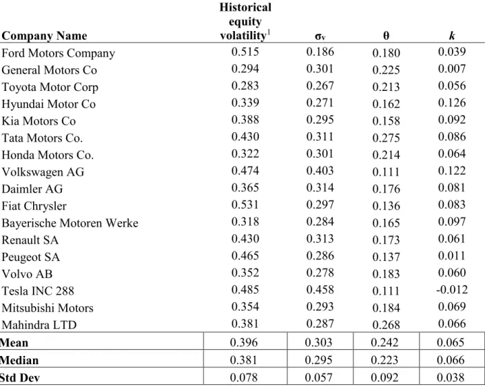
Table 6 shows a break-down of the parameters estimated using the section 3.1 model for each of the companies in the sample. Except for General Motors, σv is lower than the historical

equity volatility. This most likely happens because the estimated project volatility does not take into account the leverage of the firm. Except for Volkswagen and Tesla, σv shows a similar value

across the industry, around 30%. This isn’t the case with the historical volatility of equity, which is very heterogeneous across firms. This difference can be the result of different levels of financial leverage impacting the project risk. Furthermore, the high standard deviation the market risk is shows that the market risk differs highly from company to company. Moreover, as one can expect from a mature industry, the k estimates are all positive except for Tesla. This is likely to be the result of the company still being in its infancy. The estimated values of k aren’t consistent through the industry, though. This shows that companies’ payout rates can be very different despite having similar volatility. Conditional on the expected return on the project, a lower k implies a higher expected growth on the project value. This may be the case for firms with higher retention for research purposes or other expenditures. It may also be evidence that the hypothesis of a constant level k doesn’t hold.

34 Table 6 – Section 3.1 Model Estimated Parameters

Company Name

Historical equity

volatility1 _{σv θ k}

Ford Motors Company 0.515 0.186 0.180 0.039

General Motors Co 0.294 0.301 0.225 0.007

Toyota Motor Corp 0.283 0.267 0.213 0.056

Hyundai Motor Co 0.339 0.271 0.162 0.126

Kia Motors Co 0.388 0.295 0.158 0.092

Tata Motors Co. 0.430 0.311 0.275 0.086

Honda Motors Co. 0.322 0.301 0.214 0.064

Volkswagen AG 0.474 0.403 0.111 0.122

Daimler AG 0.365 0.314 0.176 0.081

Fiat Chrysler 0.531 0.297 0.136 0.083

Bayerische Motoren Werke 0.318 0.284 0.165 0.097

Renault SA 0.430 0.313 0.173 0.061 Peugeot SA 0.465 0.286 0.137 0.011 Volvo AB 0.352 0.278 0.183 0.060 Tesla INC 288 0.485 0.458 0.111 -0.012 Mitsubishi Motors 0.354 0.293 0.184 0.069 Mahindra LTD 0.381 0.287 0.268 0.066 Mean 0.396 0.303 0.242 0.065 Median 0.381 0.295 0.223 0.066 Std Dev 0.078 0.057 0.092 0.038

1_{Volatility has been computed using the log return of market value of equity}

Figure 2 shows an x,y plot comparing σv and the standard deviation of the YoY log changes

of EBIT (see Table 1). Ideally, if the assumptions behind the EBIT payout process hold, the trend line should be close to x=y with an origin at (0,0). This is clearly not the case. A positive trend line is observed, in part due to two clear outliers. This is likely the result of our empirical standard deviation of the log changes of EBIT being not well estimated (short time span). It can be however also the result of EBIT not following a GBM (the shapiro test was rejected in 4 out of 17 firms).

35 Figure 2: Section 3.1 σv regression against Empirical EBIT volatility

*Empirical EBIT volatility was computed by fitting a robust linear model that uses M estimators that control for outliers.

6.1.2 Parameter Estimates (section 3.1 model)

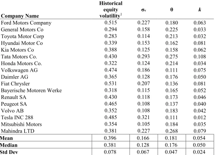
The estimates for the section 3.2 model are presented in Table 7. σv falls between 15%-20%

for most companies. Again, the average σv is much lower than the historical volatility of equity.

The difference is even more pronounced in section 3.2 model than in the section 3.1 model. By adding operational leverage to financial leverage, the asset volatility estimates have become lower. This outcome is in line with the empirical findings presented in section 5. k estimates are approximately 1 p.p. lower in this model. This implies lower probabilities of default across the industry because a lower k, if all else remains the same, would lead to a higher drift and therefore a lower default probability. Another interesting change in this model is that Tesla has now a positive estimate for k, which is more in line with the model assumptions.

y = 2,7685x - 0,3309 R² = 0,1599 0,000 0,200 0,400 0,600 0,800 1,000 1,200 0 0,1 0,2 0,3 0,4 0,5

36 Table 7 - Section 3.2 Model Estimated Parameters

Company Name

Historical equity

volatility1 σv θ k

Ford Motors Company 0.515 0.227 0.180 0.063

General Motors Co 0.294 0.158 0.225 0.033

Toyota Motor Corp 0.283 0.114 0.213 0.032

Hyundai Motor Co 0.339 0.153 0.162 0.081

Kia Motors Co 0.388 0.125 0.158 0.062

Tata Motors Co. 0.430 0.293 0.275 0.108

Honda Motors Co. 0.322 0.124 0.214 0.034

Volkswagen AG 0.474 0.186 0.111 0.075

Daimler AG 0.365 0.128 0.176 0.050

Fiat Chrysler 0.531 0.207 0.136 0.081

Bayerische Motoren Werke 0.318 0.115 0.165 0.052

Renault SA 0.430 0.118 0.173 0.046 Peugeot SA 0.465 0.108 0.137 0.040 Volvo AB 0.352 0.108 0.183 0.042 Tesla INC 288 0.485 0.321 0.111 0.012 Mitsubishi Motors 0.354 0.105 0.184 0.035 Mahindra LTD 0.381 0.227 0.268 0.079 Mean 0.396 0.166 0.181 0.054 Median 0.381 0.128 0.176 0.050 Std Dev 0.078 0.067 0.047 0.024

1_{Volatility has been computed using the log return of market value of equity}

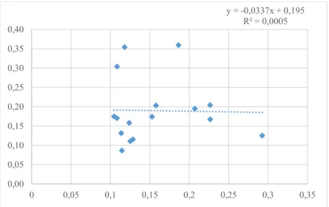
Figure 3 shows the estimated σv with the standard deviation of their corresponding YoY

log changes presented in section 5 respectively. Surprisingly, the low R2 _{shows that our empirical}

estimates are strangely uncorrelated with the volatility estimates that come out from our calibration exercise. Again, the short time span of the data and the fact that the log changes of EBIT+SGA may not be effectively normally distributed could be leading to this effect.

37 Figure 3: Section 3.2 σv regression against Empirical EBIT volatility*

*Empirical EBIT volatility was computed by fitting a robust linear model that uses M estimators that control for outliers.

6.2 Credit Risk Indicators

6.2.1 Credit Risk Indicators (section 3.1 model)

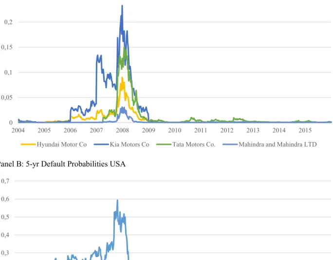
Figure 4 (Panel A to E) shows the 5-year probability of default for the period between 2004 and 2016 based on section 3.1 model. The probabilities of default presented were computed under the physical measure. Over the selected period the average default probability was 2.3% peaking at 9.04% in early 2009 and dropping to a lowest point of 0.5 % in late 2010. As expected, an uptick in default probability in all geographies is observed starting in 2008. A recovery from this event is also shown in most companies. All firms keep their 5-year PDs under 10% except for Volkswagen, Peugeot and Fiat. Panel-A shows that three of the four Asian manufacturers were affected by the crisis. Mahindra was less affected probably because its revenue streams are less related with U.S. and European markets. Panel-B shows how bad the crisis hit the industry in the U.S. with Ford breaching the 50% probability during that period. Chrysler and GM probabilities of default are not presented as these firms were both spun out into different bankruptcy salvage programs and their stock was thus unlisted. European car manufacturers, excluding Germany, show a momentary hike in default probabilities during the crisis. They do recover by 2010, but another hike in default probabilities occurs for two of the car manufactures. In contrast to these European players, German car producers were among the least affected in 2008. The exception is VW, whose 5-year probability of default jumped from close to 0 in the beginning of 2008 to approximately 8% in

y = -0,0337x + 0,195 R² = 0,0005 0,00 0,05 0,10 0,15 0,20 0,25 0,30 0,35 0,40 0 0,05 0,1 0,15 0,2 0,25 0,3 0,35

38 2009. After 2010, the probability of default of VW decreased to around 3%, but it never recovered to pre-crisis levels. The probability of default increased again in 2015 following the carbon emissions scandal. Japanese firms (Panel E) show extremely low default probabilities during the whole period. The only exception is Mitsubishi whose probability of default has a short spike during the 2008 crisis.

Figure 4: 5-yr Default Probabilities Split by Geography Panel A: 5-yr Default Probabilities Asia (Exc. Japan)

Panel B: 5-yr Default Probabilities USA

0 0,05 0,1 0,15 0,2 0,25 2004 2005 2006 2007 2008 2009 2010 2011 2012 2013 2014 2015 Hyundai Motor Co Kia Motors Co Tata Motors Co. Mahindra and Mahindra LTD

0 0,1 0,2 0,3 0,4 0,5 0,6 0,7 2004 2005 2006 2007 2008 2009 2010 2011 2012 2013 2014 2015 Ford Motors Company General Motors Co Tesla INC 288

39 Panel C: 5-yr Default Probabilities EU (Excluding Germany)

Panel D: 5-yr Default Probabilities Germany

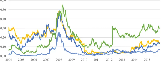
0 0,05 0,1 0,15 0,2 0,25 0,3 0,35 0,4 2004 2005 2006 2007 2008 2009 2010 2011 2012 2013 2014 2015 Fiat Chrysler Renault SA Peugeot SA Volvo AB

0 0,02 0,04 0,06 0,08 0,1 0,12 0,14 2004 2005 2006 2007 2008 2009 2010 2011 2012 2013 2014 2015 Volkswagen AG Daimler AG Bayerische Motoren Werke