Siemens AG
Equity Valuation
Bernardo Santos Silva
152113371
Abstract
This dissertation presents an in-depth analysis and consequent equity valuation of Siemens AG. The main objective of this paper is to provide an alternative perspective of what might be the fair value of this company considering its prospects of growth, risk and position in the market. The idea that value is highly subjective is kept in mind during all this process although it is important to understand how crucial this
information is to shareholders and potential investors and the necessity of maintaining a neutral position.
In order to accomplish what is purposed an overview of the most important valuation techniques and related theory is performed. This part is used as a support for many of the decisions along this dissertation.
In the end, the methods and results of this dissertation are compared with those of HSBC in one of their published reports.
Acknowledgements
The completion of this dissertation symbolizes the end of my Masters, this experience has been very rewarding not only because of the tools that were obtained that will help me through my career but also because of the opportunity to meet and learn with very interesting people, both professors and colleagues.
Regarding the last 6 months, I must express my gratitude for all the assistance and support provided by friends, colleagues and, especially my advisor, professor José Carlos Tudela Martins, whose availability and patience were crucial to the realization of this dissertation.
Finally, my acknowledgements are also sent to Jan Philipp Bellmann, from Siemens, and Michael Hagmann, from HSBC, for their assistance, material provided and especially for their solicitude.
Contents
1. Introduction ... 1
2. Literature Review ... 2
2.1 Valuation Methods ... 3
2.1.1 Relative Valuation ... 3
2.1.2 Discounted Cash Flows Models ... 5
2.1.3 Economic Value Added (EVA) ... 11
2.1.4 Option Based Valuation ... 11
2.1.5 Asset Based Valuation ... 12
2.2 Other Issues on valuation ... 13
2.2.1 Risk free ... 13
2.2.2 ERP ... 13
2.2.3 Beta ... 14
2.2.4 Cross Border and Conglomerates Valuation ... 15
2.3 Conclusion ... 16
3. Internal Analysis ... 17
3.1 Presentation ... 17
3.1.1 Performance Indicators and Stock Performance ... 18
3.1.2 Strategic Vision ... 20
3.1.3 Shareholder Structure ... 21
3.1.4 Siemens Rating ... 21
3.2 Dresser-Rand ... 22
3.2.1 The Deal ... 22
3.2.2 Presentation and Analysis of the Company ... 22
4. External Analysis ... 24
4.1 Macroeconomic Analysis ... 24
4.2 Sector and Market Analysis ... 24
5. Valuation ... 26
5.1 Methodology ... 26
5.2 Forecasting and Other Assumptions ... 27
5.2.1 Revenues ... 27
5.2.2 Cost Structure and other Income ... 28
5.2.4 Working Capital ... 30 5.2.5 Taxes ... 31 5.2.6 Debt ... 32 5.2.7 Financial Statements ... 33 5.3 Dresser-Rand Valuation ... 35 5.4 Discount Rates ... 36 5.5 APV Valuation ... 37
5.5.1 Unlevered Value of Operations ... 37
5.5.2 Interest Tax Shields (ITS)... 38
5.5.3 Bankruptcy Costs ... 39 5.6 Multiple Valuation ... 40 5.7 Sensitivity Analysis ... 41 6. Valuation Comparison... 44 7. Conclusion ... 47 8. Appendix ... 48
8.1 Historical Income Statement ... 48
8.2 Historical Balance Sheet ... 49
8.3 Forecasted Income Statement ... 50
8.4 Forecasted Balance Sheet ... 51
8.5 Sales by Region ... 52
8.6 Historical Effective Tax Rate... 52
8.7 History of Credit Ratings ... 52
8.8 Criteria for Remaining Financial Statements Items ... 53
8.9 Moody’s Probability of Default ... 53
8.10 Siemens’s Peer Group ... 54
8.11 Dresser-Rand’s Peer Group ... 55
8.12 Executive Summary ... 56
9. References ... 58
9.1 Academic References ... 58
1
1. Introduction
This dissertation puts in practice what has been taught in classes during the last year, regarding Equity Valuation. The subject chosen was Siemens A.G, the biggest industrial conglomerate company in Europe and one of the biggest in the world.
The focus of this dissertation is to determine a target price for the company and
compare the results with the ones from an investment bank. The purpose of this will be to identify the methodological differences among them and explain the different sources of value.
The structure of this dissertation is organised in 5 main sections: Literature Review, Internal Analysis, External Analysis, Valuation and Comparison of Results. This order intends to follow the same one that was used in the process of doing this valuation.
1. The Literature Review presents the most relevant studies and papers regarding valuation methods and other related issues. Also, along this section, some decisions concerning the methodology of the valuation are provided and justified;
2. In the Internal Analysis, the company’s identity, structure and recent
performance are examined in order to better forecast what might be its future; 3. The External Analysis intends to provide a picture of what is the environment in
which Siemens is in. The focus is both on industry and Macro analysis;
4. The Valuation, the most crucial part of this dissertation, intends to explain all the steps from the forecasting to the target price determination. The reasoning behind the assumptions made was based on the insights provided by the first 4 sections combined with the best of judgement of the author;
5. In the Comparison of Results is where the Investment Bank results are analysed and faced against the results of this dissertation in order to understand which causes are behind those differences. The investment Bank chosen is the HSBC Bank PLC.
2
2. Literature Review
This section has the role to go over the techniques and particularities in the valuation of a company by presenting the most relevant papers and their respective perspectives about each subject.
In order to understand what value is and why it is important to assess it, Fernandez (2007) makes a very important distinction between value and price. He defines price as “the quantity agreed between the seller and the buyer in the sale of a company”. This differs from value because it concerns the perception of each player in the market, considering that each one values the company differently. This means that, in practice, the seller, the buyer or even both had to compromise in order to get to an agreement due to the fact that they are in different positions and have opposite interests.
According also to Fernandez (2007), valuation can be done with several purposes: set the minimum price for an acquisition; decide to sell or buy publicly traded stock; determine price for an IPO; create systems of compensation based on value creation; identify value drivers; and assist strategic decisions.
Reinforcing the differences in the perception of value, is the increasing number of valuation techniques which contribute to a more diverse and complex universe of estimations. Damodaran (2006) recognizes that these models make very different assumptions about what determines value, although, he thinks they share common characteristics. Considering this, now, the focus will be in presenting each valuation method along with some related issues. Also, I will reveal and explain, along this section, some of the choices made for valuing Siemens.
3
2.1 Valuation Methods
2.1.1 Relative Valuation
Relative Valuation or Multiples Valuation is a technique based on the assumption that the market is efficient and that similar assets have similar values. Damodaran (2006) identifies three steps to perform a valuation using multiples:
1. Find comparable assets that are priced by the market; 2. Scale the market prices to a common variable;
3. Adjusting for differences across assets.
First, comparable assets can be identified according to different criteria. A very common choice is to use an industry classification system such as SIC (Standard
Industrial Classification). Eberhart (2004) is one of the few researchers to devote time to this specific topic by comparing a wide variety of classification systems publicly
available. Although it seems logic that companies’ profiles vary a lot within an industry, it also makes sense that companies that compete in the same markets and are subject to the same set of macroeconomic forces can be target of comparisons. Another alternative is to look at the fundamentals of a company. Damodaran (2006) defines a comparable company as one with growth potential, risk and cash flows similar to the firm being valued, highlighting the fact that there is no industry or sector reference in this
definition. These two perspectives of what is a comparable company can be combined as Bhojraj, lee and Ng, (2003) does by selecting companies on the basis of variables that drive the cross-sectional differences in a certain ratio, including profitability, growth and the cost of capital. Finally, Andrew W. Alford findings on his paper about “The
Effect of the Set of Comparable Firms on the Accuracy of the Price-Earnings Valuation Method” reveal that much of the cross-sectional variation in P/E (Price-to-Earnings) that
is explained by risk and earnings growth is also explained by industry and that the selection of companies solely on the basis of the fundamentals is not advantageous. Even though we may have a quite strong peer group, there is always the need to find a common variable as measure of comparison because even similar companies differ in size, number of shares, capital structure and other parameters. To avoid a direct comparison, multiples are used based on different variables:
4 - Earnings (PE, EV/EBITDA, PEG) - Assets (P/BV)
- Cash Flows (P/CF, EV/Operating FCF, etc…) - Revenues (P/Sales)
- Industry Specific (EV/Subscriber, EV/Reserves, EV/Capacity, EV/Invested Capital, etc…)
Although “there is no clear-cut answer for which multiples should be used, many researchers tried to evaluate their accuracy” (Kim and Ritter, 1998). There is studies that show that, in practical life, investment bankers typically use multiples as a main technique or as assistance to other techniques. Fernandez (2001) shows that the PE and Enterprise Value-to-EBITDA appear in first and second, respectively, as the valuation methods most widely used in Morgan Stanley for valuing European companies, whereas the DCF (Discounted Cash Flow) method only appears in fifth place. Lie and Lie (2002) also supports this trend.
Regarding empirical studies, the opinions are diverse. Liu, Nissim and Thomas (2002) found that multiples derived from earnings are more accurate than the ones from cash flow, book value of equity and sales. Contrarily to this, Lie and Lie (2002) considers that asset value multiples (E/BV) yield the best results. Even so, these two papers agree on the fact that the use of forecasted performance instead of the historical performance increases the efficiency of the earnings multiple.
Lie and Lie (2002) also finds that EBITDA multiple generally are more accurate than EBIT multiple and that accuracy and bias between multiples vary by company size, profitability and sector.
Once an analyst has chosen his peer group and the right multiples, he needs to decide how to properly apply the multiple. Most relative valuations compute the average of each multiple of the comparable companies which opens some space for discussion on how to do it. Liu Nissim and Thomas (2002) found that the harmonic mean improves the valuation comparing to arithmetic mean and median. Also, Beatty, Riffe and Thompson (1999) state the same but only regarding multiples of earnings, book value and total assets.
Another measure used by analysts is the adjustment for the growth rate, known as P/EG or EV/EG depending if it is based on PE or EV/EBITDA. Fernandez (2001) explains
5
that these adjusted multiples are used mainly in growth industries since the growth expectations vary a lot.
Regarding this valuation, I intend to use the sum-of-the-parts method adapted for multiples suggested by Damodaran (2009). In his paper, he presents some alternatives to value conglomerate companies. This specific method consists on valuing the different businesses separately by finding “Pure Play” companies for each peer group. The results provided by each business’s relative valuation is weighted by their respective sales and summed up.
I consider this method the most appropriate one for valuing Siemens giving the level of detail provided in their financial information. Also, by using different peer groups, makes it possible to grasp the fundamentals behind each industry in terms of market growth and risk.
2.1.2 Discounted Cash Flows Models
It is consensual that DCF method is the one that provides the strongest theoretical support to a valuation. This is because “The value of an asset is not what someone perceives it to be worth but it is a function of the expected cash flows on that asset” (Damodaran, 2006). By following this reasoning, high valuations are synonym of high and stable (or growing) cash flows.
At this point, we are presented with many different methods all of them using
discounted cash flows. Fernandez (2002) presents 10 methods to value a company, also Damodaran (2006) refers to 7 methods grouped in 4 classes. In order to avoid being too extensive on this subject, in this paper, I will focus on these main DCF methods:
Free Cash Flow to the Firm (FCFF) Free Cash Flow to the Equity (FCFE) Dividend Discount Model (DDM) Adjusted Present Value (APV) Economic Value Added (EVA)
6
These alternatives are consistent between them and are supposed to arrive to the same value although “they differ only in the cash flows taken as the starting point for the valuation” (Fernandez, 2002). Two important components of these models are the Cost of Capital, or discount rate, and Terminal Value which I will start by introducing.
Cost Capital
Using a discount rate to adjust cash flows has become a very popular method to account for risk. An alternative to this would be to use the certainty equivalent approach where the cash flows are adjusted and then discounted at the risk free rate.
Depending on the type of cash flows that are being used, the discount rate used differs accordingly. This means that when using cash flows originated by the whole firm we must use a discount rate that represents both equity and debt required returns (WACC) although when considering only the equity cash flows, the most appropriate is to use the cost of equity.
The WACC represents the cost of capital of a firm although Fernandez (2010) points to a common mistake which is to think of WACC as a cost or a required return when it is no more than a weighted average of those two.
The traditional approach to calculate it is:
𝑊𝐴𝐶𝐶 𝑎𝑓𝑡𝑒𝑟 𝑡𝑎𝑥 = 𝐾𝑒 × 𝐸𝑞𝑢𝑖𝑡𝑦 𝑉𝑎𝑙𝑢𝑒
𝐸𝑛𝑡𝑒𝑟𝑝𝑟𝑖𝑠𝑒 𝑉𝑎𝑙𝑢𝑒+ 𝐾𝑑 ×
𝐷𝑒𝑏𝑡 𝑉𝑎𝑙𝑢𝑒
𝐸𝑛𝑡𝑒𝑟𝑝𝑟𝑖𝑠𝑒 𝑉𝑎𝑙𝑢𝑒× (1 − 𝑡)
Where: Ke - Cost of Equity, Kd - Cost of Debt and t - Tax Rate.
Then, in order to compute it, we need to have information on the cost of equity and debt, capital structure and tax rate. Some of this information is not directly available and it needs to be calculated.
However, there is a limitation in this approach since it does not consider a varying capital structure. In order to overcome it a manager or analyst can either assume a target capital structure (Miles & Ezzel, 1980) or adjust the capital structure by calculating a new WACC continuously over the explicit period. (Harris & Pringle, 1985).
7 Terminal Value
Considering that a company can last for an indeterminable period of time, it is assumed that it has infinite lives. Since it is not possible to calculate cash flows for that amount of time, an explicit period value and a terminal value must be computed. This last value is treated as a perpetuity and it is assumed to have a constant growth rate which,
according with Damodaran (2006), it should be lower or equal than the growth rate of the economy in nominal terms.
FCFF (Free Cash Flow to the Firm)
Using this method, we are valuing the whole firm by discounting the cash flows generated by the company before any claims by the investors. As a discount rate, it is used the weighted average of the cost of equity and debt after taxes (WACC after-tax). This model was first developed in 1958 by Modigliani and Miller and states that the value of a firm can be extracted by calculating the present value of the after-tax
operating cash flows. From the several definitions of operating cash flows, the FCFF is the most widely used:
FCFF = After-tax Operating Income + Depreciation – Capital Expenditures - ∆ Net Working Capital
This cash flow after taxes represents the remaining in cash for the investors, either debt or equity. Damodaran (2006) says that the most revolutionary idea behind firm
valuation is that equity investors and debt holders are ultimately partners who finance the firm and share in its success.
Even though the purpose of this method is to extract the value of a firm, there is the possibility of finding the value of Equity by subtracting all the non-equity claims, including debt and financial leases.
FCFE (Free Cash Flow to the Equity)
Contrarily to the previous method, this one is used to extract directly the value of equity and it can be done using the FCFF by deducting the non-equity expenses and
8
FCFE = FCFF - Interest expenses after taxes – (Debt Issued - Debt Repayments) Then, this cash flow can be interpreted as the left over after all reinvestment needs and debt repayments (Damodaran, 2006).
The discount rate used for these cash flows changes comparing with FCFF method since it should represent only the cost of equity.
DDM (Dividend Discount Model)
This model is probably the most intuitive one since it focuses on the two sources of cash flow from a share, dividends and price (that is reflected, in theory, by the present value of future dividends). It can be computed by using the Gordon growth model:
𝑃𝑛= 𝐷𝑃𝑆 𝐾𝑒 − 𝑔
In case there are stock buybacks, this value should be added as dividends. The fact that it requires such simple assumptions makes it a very straightforward model to use. However, there are limitations associated with DDM since dividend policies vary quite much between companies. On one end, there are companies that hold back cash and pay few or no dividends and, on the other end, companies that pay more dividends than they have available on cash flows. This diversity makes it very difficult to compare
companies through this method.
Notwithstanding, Damodaran (2006) specifies three scenarios where DDM can be useful: to establish a floor value for firms with higher cash flows than dividends; in the valuation of companies that have a dividend pay-out ratio equal to 1; and when cash flow estimation is very uncertain and the dividends are the only cash flows that can be estimated.
APV (Adjusted Present Value)
Damodaran (2006) explains it as an approach that attempts to estimate the expected value of debt benefits and costs separately from the value of the operating assets. This is achieved by discounting the tax shields and estimating the bankruptcy costs associated with debt. At the same time, the value of the company without debt is calculated. Then, value of a firm will be:
9
Firm Value = Value of Firm without Debt + (Tax Shields – Bankruptcy Costs)
The logic behind it is that for each amount of debt that a company adds to its financial structure there are benefits (interest tax savings) and costs (expected cost of bankruptcy) associated with it. Thus, by separating from the firm value the effects of borrowing money we know how much value it creates to the all company.
Tax Shields
As it was said, Tax Shields, are the tax benefits from having debt. For a company that is expected to maintain its capital structure over time, the present value of tax shields is given by:
𝑃𝑉 (𝑇𝑎𝑥 𝑆ℎ𝑖𝑒𝑙𝑑𝑠) = Interest x Debt x Tax rate 𝑈𝑛𝑙𝑒𝑣𝑒𝑟𝑒𝑑 𝑐𝑜𝑠𝑡 𝑜𝑓 𝑐𝑎𝑝𝑖𝑡𝑎𝑙
Although it is consensual that this is how the tax shields are calculated there is some discussion around three issues, whether the amount of debt can change over time, the discount rate and the tax rate used. At first, when APV method appeared it was considered that both debt amount and tax rate were constant and the discount rate should be the pre-tax cost of debt. Since then, some variations to the model were proposed, considering variations in the tax rate and level of debt but it is around the discount rate used that much of the divergence is.
According with Fernandez (2002), there is nine theories on how to calculate the value of Tax Shields (VTS):
Where: D – Value of Debt, T – Corporate Tax Rate, Ku – Unlevered cost of capital, Kd – Cost of Debt and Rf – Risk-free rate
Source: Fernandéz, Valuing Companies by Cash Flow Discounting: Ten Methods and Nine Theories, 2002
Theory Value of Tax Shields
Fernandez (2004) DT Damodaran DT-[D (Kd-Rf) (1-T)]/Ku Practinioners D[Rf-Kd(1-T] /Ku Harris-Pringle TD Kd/Ku Myers DT Milles-Ezzell TDKd (1+Ku)/[(1+Kd)Ku] Miller (1997) 0
With Costs of leverage D(KuT+ Rf-Kd)/Ku
Modigliani-Miller DT
10
Fernandez (2002) states that VTS should be the difference between the tax expenses of the unlevered company minus the tax expenses from the one with leverage. As a consequence it should be discounted with Ku, which contrasts the reasoning from past authors. Authors like Myers (1974), Miles and Ezzel (1980), Harris and Pringle (1985) and Cooper and Nyborg (2006) support that cost of debt should be the right discount rate to use, although with some difference in their models since, for example, Miles and Ezzel believed that it should be used the Kd for the first year and Ku for the rest of the period.
Bankruptcy Costs
This component is sometimes not considered by authors and analysts given the
difficulty to estimate a reliable value. In theory, the costs of bankruptcy are composed by indirect and direct costs and to estimate its value we must use the probability of default correspondent to the level of existent debt.
PV of Bankruptcy costs = Probability of default x PV (Bankruptcy costs)
Although, in practical life, it becomes very hard to estimate either the probability of default or the bankruptcy costs. Some studies have tried to come up with evidences about the weight of bankruptcy costs. Andrade and Kaplan (1998) that concluded that indirect costs accounted for 10-23% of firm value. Also, Damodaran (2002) believes that both indirect and direct costs represent 30% of firm value.
Another relevant paper on this matter is the one from Kortweg (2007), where he estimates the ex-ante costs of financial distress across industries, based on the market opinion. The results showed that the market expect these costs to vary between 0 and 11% of firm value. Also, the author found that companies choose their level of leverage taking into account the trade-off between tax benefits and costs of financial distress. This method has as a main weakness the fact that it is hard to include a good estimation of the bankruptcy costs and the alternative of not accounting for them is not ideal also. Notwithstanding, the adjusted Present Value method is definitely appreciated within the researchers community given its flexibility and detail, Luehrman (1997) says “APV always works when WACC does, and sometimes when WACC doesn’t, because it requires fewer restrictive assumptions”.
11 2.1.3 Economic Value Added (EVA)
EVA is one of many excess return models and the most widely used among them. Damodaran (2006) defines it as “a measure of the surplus value created by an
investment or a portfolio of investments”. In other words, it represents the excess return on an investment. It can be calculated by following formula:
Economic Value Added = (Return on Capital Invested – Cost of Capital) X (Capital Invested)
The underlying logic in this formula is the same for NPV. The value of EVA discounted over the years with the cost of capital should give a similar value to NPV.
Damodaran (2006) points out some possible missteps regarding the calculation of ROIC, Capital Invested and Cost of Capital. Namely, the older the firm the bigger is the amount of adjustments that book value values require.
2.1.4 Option Based Valuation
This method has appeared in response to companies with “projects that involve both with a high level of uncertainty and with opportunities to dispel it as new information becomes available” (Kopeland and Keenan, 1998). These kinds of projects include a range that goes from a development of a new product to the exploration of an oil field. For these companies, opportunities are the most valuable thing they own (Luehrman, 1997). Moreover, this method appearance is related with some criticism to the most traditional methods, like DCF, regarding its lack of flexibility (Luerhman, 1997) and tendency to underinvestment and stagnation (Kopeland and Keenan, 1998).
According with Luerhman (1997) the right to start, stop, or modify a business activity at some future time has to be incorporated in the valuation. It is different to take these decisions now or in the future, especially when we might have new and more reliable
12
information about the subject. Thus, “the option valuation recognizes the value of learning” (Leslie and Michaels, 1997).
The models of option pricing used are Binomial Model and Black-Scholes Model, being the second, the most important one but also the most complex. Managers are known to avoid using it since the mathematics behind Black-Scholes formula are not accessible to the standard management knowledge. Although, Leslie and Michaels (1997) believe that in the same way as managers used CAPM, without a deep knowledge of the subject, they can also use Black-Scholes.
Even though these authors recognize the added value of this approach, they look at it as a complement to a valuation without discarding the traditional methods. Also, they point a limitation which is the fact that to use option-based valuation requires information, knowledge and the vision of top managers. This demand makes it very hard for external investors to use it.
2.1.5 Asset Based Valuation
This method follows the belief that the value of assets individually might be a better proxy of the true value of a firm than the DCF valuation that is based in dubious assumptions.
There are three different approaches to do an asset based valuation: Book Value; Replacement Cost; and Liquidation Value. The first one, Fernandez (2007) defines it as the value of shareholders’ equity reported in the balance sheet which is the difference between total assets and liabilities. The second, also called Substantial Value, represents the amount needed to create a company with the exact same assets. The Liquidation Value, as its name says, is the value obtained from selling all the assets now.
Theoretically, this value should be similar to the value of the discounted cash flows of the individual assets although we should account for the discount on the value that exists in the urgency of selling (Damodaran, 2006).
However, when using an asset based method the prospects of growth are not being considered. Only information about the past and the present is incorporated. This may not have a big effect on the valuation of a company in a mature market and that is composed predominantly by fixed assets. Although using it for companies with growth
13
opportunities and potential for excess returns will produce a very different value from the true value (Damodaran, 2006).
2.2 Other Issues on valuation
2.2.1 Risk free
In Damodaran (2008), the author focuses on the “Basic Building Block” of a valuation which is the risk-free rate. The importance of this component is explained in this paper as being the start for every valuation because it is through the risk-free rate that we find both cost of equity and debt.
It is consensual that the risk-free rate should be the expected return of an asset with no default risk and because of that government bonds are widely used to represent this rate although there are several countries that present default risk.
According to Damodaran (2008), the maturity chosen for the government bond matters since it should correspond to the period in which you are going to account for cash flows.
Also, the rate should be in real terms since we do not want that the growth derived from inflation prices misrepresents the valuation.
For the purpose of this dissertation, the 10 year German government bonds will be used as the risk-free rate.
2.2.2 ERP
The expected return of an investment can be divided in two components, the risk-free rate, discussed in the previous topic, and the risk premium which compensates for the risk attached to the specific investment. Damodaran (2012) defines equity risk premium as the “premium that investors demand for the average risk investment, and by
extension, the discount rate that they apply to expected cash flows with average risk”. In the same paper, Damodaran defines the determinants that influence ERP: Risk Aversion; Economic Risk; Information disclosure and transparency; Liquidity; Catastrophic risk; Government policy; and behavioural component.
The most widely adopted approach to estimate equity risk premiums is by using the historical ERP although there is a significant criticism about this approach where
14
Fernandez (2006) says that historical ERP is not equal to required ERP which is different for each investor. Also, when it comes to deal with less developed markets than U.S or some European countries there are limitations about the historical data available (Damodaran 2012).
Damodaran (2012) presents two alternative approaches. The first, consists in using a survey where managers and investors are asked about what are their expectations of returns in equity. The second approach estimates implied premiums by using market rates and prices on assets traded today. These two alternatives to get the ERP correct some of the limitations regarding the historical approach but present other kind of problems as overweighting recent history.
In order to determine the cost of equity of Siemens, I will use ERP for Germany provided by Damodaran considering that there are no recent studies on the matter that provide better estimates.
2.2.3 Beta
When using the CAPM to estimate the cost of equity of a firm, the component, along with ERP, that creates more problems is beta. It can be defined as a measure of the systematic (or undiversifiable) risk of an asset. In other words, represents the relation between the returns of a specific asset and the ones from its market.
According with Damodaran (1999), betas have two basic characteristics, the first, is that they add on to a diversified portfolio, rather than total risk. Second, is the fact that they measure the relative risk of an asset.
Since there is no efficient portfolio that represents the whole market, most practitioners use market indices which include only a subset of securities. S&P 500 is the most commonly used proxy for beta estimation for US companies and it only considers 500 companies. If we tried to estimate the beta for emerging markets we will have a much harder scenario given the existence of few public companies and short historical data. Damodaran also presents three issues to take into account when estimating betas:
o Choice of Market Index – indices that include more securities should provide better estimates, as should the ones that are market-weighted.
o Choice of a Time Period – By using longer time periods we may get more observations but this may adulterate the final results if the company has suffered several changes in their characteristics in the past.
15
o Choice of a Return Interval – By using shorter intervals it is likely to create some bias due to the fact that assets are not traded on a continued basis. On the other side, the use of bigger intervals may reduce significantly the number of observations if the company has a recent public history.
When analysing betas across industries it is clear that there are considerable differences. This happens mainly because of the “statistical noise” reduction that a narrower industry specific market index provides comparing with a general one. Kaplan and Peterson (1998) call a “Pure Play Portfolio” to a portfolio composed by companies with one business and defend that this kind of portfolio is ideal to get a precise beta, although they recognize the difficulty in finding a large sample of this type of companies. Also, the author found that large market-capitalization firms (most of them
conglomerates) tend to have smaller betas than those in small market-capitalization firms.
For this purpose, I have used the historical beta of Siemens using DAX Index as
portfolio. The nature of Siemens, i.e. having a diversified portfolio of businesses makes this acceptable since this company is exposed to many industries and their specific risks. Also, the monthly data used was from a period of 3 years ending in February 2015. The choice of the period length takes into account a period where the company remains fairly stable in terms of portfolio and leverage.
2.2.4 Cross Border and Conglomerates Valuation
Multinationals may not represent a large percentage of the overall number of firms, they have an outsized influence, because they tend to be the largest firms (in terms of
revenues, earnings and market capitalization) in many markets.
These companies, due to their presence in different countries, cannot be valued in the same way as the ones that are only exposed to the political and economic risk of one country. One way to solve this problem is valuing the company using the sum-of-the-parts approach. Alternatively, we can adjust only the risk parameters using a weighted average in order to estimate the risk for the consolidated company.
Also, there are other issues besides risk. Centralized costs and Intra-company
transactions have to be looked out for to avoid the inflation of sales and its respective costs. Finally, the effective tax rate of a multinational is just a reflection of the multiple taxes rate along the countries it is operating in, which demands for attention.
16
2.3 Conclusion
After looking over the most important literature on Equity Valuation and analysing the target company, I have decided to use as main valuation technique the DCF with the Adjusted Present Value approach. I believe the APV can extract a reliable value considering the fact that the company has not maintained a constant capital structure due to the big variations of cash. As a downside, there is the calculation of Bankruptcy costs which will have to be handled using the studies that were mentioned earlier even though considering this is not most ideal solution.
In order to make this valuation more consistent with the current market context I will also value the company using a variation of the sum-of-the-parts multiple valuation to support the main method. The choice of this particular technique is due to the
diversified portfolio of businesses that Siemens is in and the limited number of direct peer companies existent.
Damodaran (2009), when valuing conglomerate companies, suggests two approaches, the one where the company is valued as a whole and the one where the company is broken down into businesses and those are valued separately (the sum-of-the-parts approach). Even though the second approach might be the correct in theory it also requires a great deal of assumptions regarding the allocation of assets and profit to the respective businesses. Considering this, I have decided to value the company as a whole given the short level of detail provided and also the fact that Siemens’s businesses, with the exception of Healthcare, are interrelated and positioned along the same value chain.
17
3. Internal Analysis
3.1 Presentation
Siemens AG is a German company and it was founded by Werner von Siemens in 1847. At the time, the focus was in telecommunications, since then, Siemens has
internationalized and diversified into more business areas. At the moment, this firm operates in more than 200 countries, has 343,000 employee and is organized in 8 reportable divisions, the Healthcare business, that is now managed separately, and a segment of Financial Services, which act as a partner with those divisions and also with external customers (Fig. 1). For the purpose of this dissertation, I will use the sector organization that was used prior to the current one. It was composed by only 4 sectors: Energy, Healthcare, Industry and Infrastructures & Buildings. As it can be seen in Figure 3, in 2014, Energy sector was the one that assumed the most relevance, followed by Infrastructures & Cities and Industry.
Figure 1: Business Segments Grouped along the Value Chain of Electrification
Source: Siemens Annual Report 2014
In Siemens, they define themselves as a “global powerhouse in electrical engineering and electronics”, positioning along the value chain of electrification. Its customers come from industries as distinct as Oil, Healthcare, Construction and Transportation.
18
Source:Siemens Annual Report 2014
In terms of geography, this company is divided into 3 major regions: Europe, C.IS1, Africa and Middle East; Americas; and Asia and Australia. In terms of volume of sales, by looking to Figure 2is clear that the region of Europe, C.I.S, Africa and Middle East, when including Germany, represents the majority of revenues in which the European market stands out.
3.1.1 Performance Indicators and Stock Performance
Source: Siemens Annual Report 2014
1 Commonwealth of Independent States
Million Euros 2011 2012 2013 2014
Sales 73 275 78 296 73 445 71 920
Energy 24 390 27 302 26 425 24 380
Healthcare 12 463 13 600 12 626 12 401
Industry 18 124 18 872 15 256 15 346
Infrastructure & Cities 16 166 16 731 17 149 18 291
Other 2 132 1 791 1 989 1 502 Orders 86 055 77 822 80 383 79 530 Gross Margin 33,7% 31,9% 31,2% 32,2% EBITDA margin 14,6% 12,5% 11,0% 12,7% EBIT Margin 11,3% 9,0% 7,2% 9,4% Profit Margin 8,6% 5,9% 6,0% 7,7% ROE 20,5% 14,3% 14,6% 18,2%
Book value D/E 17,0% 31,4% 39,3% 41,0%
Interest Coverage ratio 4,82 4,08 6,75 8,81
ROCE 15,8% 13,1% 9,5% 12,0% Dividend payout 42,8% 56,7% 59,1% 50,4% 34% 17% 22% 26% 1%
Figure 3: Revenues by Sector Energy Healthcare Industry Infrastructure & Cities Other
Table 2: Performance Indicators 39%
15% 8% 18%
20%
Figure 2: Revenues by Geographic Segment
Europe, C.I.S, Africa, Middle East (excluding Germany) Germany
Americas (excluding U.S) U.S
19
This table aims to resume the recent performance of Siemens using some key indicators. In terms of sales, Siemens has been inconstant since they have been going through several acquisitions and divestitures due to their strategic readjustment. The level of orders has not followed any clear trend, even though, it presents a decrease in the last 4 years. When breaking down into sectors, Infrastructures & Cities stands out from the other sector with a constant positive growth along these years. Offsetting this uptrend, the Energy and Industries sectors have been in decline. Looking at the profitability in the last 4 years, specifically to the margins and ROE, it is clear that Siemens had 2011 as its most profitable year. Since then, it has been decreasing its profitability, although this seems to be recovering when looking to 2014. Regarding their debt levels, in 2011 they had €17,940 million in debt with a book value debt-to-equity ratio of 17%. Four years later, it reached €20,940 million with a book value gross debt-to-equity of 41% where mostly was due to the decrease of excess cash. Despite this increase in leverage, the interest coverage ratio has reached the highest value of 8,81x. Finally, the dividend policy has been consistent along these years, which also has been combined with the repurchases of shares.
Siemens, AG is listed in Deutsche Börse since 1899, having delisted from NYSE on May 2014. Since then, it is only traded over-the-counter using ADR’s (American Depositary Receipts). The ticker used in the German Stock Exchange is SIE.
Source: Bloomberg
In February 2015, Siemens market capitalization was €83,019 million with 835 million shares traded in the market. As it can be seen from the graph, the share price has followed a growing trend, with an increase of roughly 40% since 2012 until now. Following an inverse trend is the dividend yield, this performance is mainly caused by the increase of the stock price as it can be seen from the table below.
60 € 65 € 70 € 75 € 80 € 85 € 90 € 95 € 100 € 105 € A ug -12 O ct -12 D ec -12 Fe b-13 A pr -13 Jun -13 A ug -13 O ct -13 D ec -13 Fe b-14 A pr -14 Jun -14 A ug -14 O ct -14 D ec -14 Fe b-15
20
Table 3: Dividend Policy
Source: Siemens Annual Report 2014
3.1.2 Strategic Vision
In the last decade, Siemens has been changing their strategic focus. In 2008, the telecommunications business had been completely divested, on the other side, investments in the renewable energies and healthcare were made.
Since last year, after the entry of the new CEO, Joe Kaeser, a new strategic plan called “Vision 2020” was launched, in response to the last years of underperformance by the company. This plan aims to put Siemens back on the path of growth and it lays on three major components:
o Focus on opportunities of growth along electrification, automation and digitalization and exit from underperforming businesses;
o A flatter and flexible structure, increasing efficiency, by eliminating layers of management;
o Achieving long-term success by supporting an “Ownership Culture” where more employees are also shareholders.
In order to deliver it, they established three phases:
Source: Siemens Annual Report 2014
Also, Siemens has linked the success of this plan to some specific goals: o Cut costs by 1 Billion € until 2016
o Increase capital efficiency target – achieve a ROCE of 15% to 20%
Million Euros 2007 2008 2009 2010 2011 2012 2013 2014
Dividends 1 292 1 462 1 380 1 388 2 356 2 629 2 528 2 533
Payout ratio 38% 24% 61% 60% 43% 57% 59% 50%
21
19% 11%
6% 64%
Figure 6: Shareholder Structure
Private Investors Unidentified Investors Siemens family Members Institutional Investors
o 30% of Division and Business Unit managers to be base outside Germany by 2020
o Increase the number of employee shareholders by 50%
3.1.3 Shareholder Structure
Source: Siemens’s website
Currently, Siemens has issued 881.000.000 registered shares of which 89% are free float since either treasury shares and Siemens family members’ holdings are considered non-free float.
3.1.4 Siemens Rating
The ratings given to Siemens are A1/stable/P-1 and A+/ stable/A-1+ by Moody’s and Standard & Poor’s, respectively. In the case of Moody’s, the last update occurred in February 2015, prior to that the rating was Aa3/Neg/P-1. The recent history of the rating of this company is in detail in the Appendix 8.7.
22
3.2 Dresser-Rand
3.2.1 The Deal
Siemens announced on September 2014 that it had come to an agreement to buy Dresser-Rand, the initial offer was $7,600 million (€5,800 million as of this date) in cash, or $83 per share with the assumption of debt.In addition to this, this deal has a ticking fee feature where, starting in March and until the deal closes, a $0.55 monthly fee will be added to the original price. At the date of this work, the European
Commission is still performing an in-depth investigation in order to assess the effects in competition that this deal may cause. The possibility that this deal does not go through will cost to Siemens $400 million in break fees excluding any other additional cost already occurred.
The synergies that the company expects to extract, reach €1,300 million until 2019. The source of these synergies is both from revenues and costs.
This company is quoted in NYSE and the recent performance of the stock has shown a sharp growth where most of it was caused by the announcement of the merger, growing 22% during the 10 days after the communication. This sign combined with the negative reaction in Siemens stock price, indicates clearly that the investors see this deal as being overpaid.
3.2.2 Presentation and Analysis of the Company
Dresser-Rand is a company that provides products and services to the Oil & Gas industry and it comes as a strategic fit to Siemens’s sector of Energy. Its headquarters are located in Huston, Texa, USA. The client base comes from more than 150 countries where 32% and 24% of the $2,812 million in revenues in 2014, came from North America and Europe, respectively.
Source: Siemens’s website
Million Euros 2011 2012 2013 2014
Revenue 2 312 2 736 3 033 2 812
Gross Margin 15% 25% 24% 27%
EBITDA Margin 5% 13% 15% 14%
Profit Margin 2% 5% 3% 5%
Book Value Debt Ratio 33% 31% 34% 31%
Coverage Ratio 4,20 5,58 6,84 5,54
ROE 12% 18% 14% 9%
23
When looking more closely to the company’s performance, it is possible to see that, in the last 4 years, there was a growth of 22% in revenues even though there was a decline of 7.3% in 2014. In terms of profitability, Dresser-Rand has shown an improvement in some indicators (Gross and EBITDA margins) although ROE has been very unstable over the last 4 years.
Regarding the capital structure, the company has, as of December 2014, a book value debt ratio of 68.9%, having decrease from 84.3% in 2013. The coverage ratios in 2013 and 2014 were 10x and 8x, respectively. The current rating from Dresser-Rand is Ba2 and BB for Moody’s and S&P, respectively.
24
4. External Analysis
4.1 Macroeconomic Analysis
Siemens as one of the most geographically dispersed companies in the world is
dependent of the macroeconomic environment at a global level. Also, given the industry it operates, there is a significant correlation between GDP growth and the performance of the company where the gross fixed investment and manufacturing value added assume a great importance.
The previsions for global GDP, in real terms, are 3% for 2015 and an average growth of 3.2% until 20202. For inflation, it is expected to reach 2.3% in 2015, and 2.5% each year until 2020. In the Eurozone, inflation is expected to grow, on average, 1.1%3. One other important factor that will influence the possible outlook of Siemens is the price of certain commodities, more specifically aluminium and copper. This happens because they account for an important part of raw material used in the final products of the company. The prices of those commodities are expected to decrease, in real terms, 3% and 6% for aluminium and copper, respectively4.
4.2 Sector and Market Analysis
This section analyses the company by sector explaining which products and services they provide, the recent performance and what can be expected from the future. This last part is based on the few studies and reports available for consultation regarding the outlook for the next 5 to 6 years.
Energy
For this sector, Siemens offers turbines and other components to oil, gas and renewable energies infrastructures. At the moment, renewable energies segment represents 28% of the revenues of this sector being the one showing a better growth. Until 2020, it is expected that the whole segment will grow 5.7% annually5.
2 “ATK Global Economic Outlook 2014-2020” – AT Kearney (2014) 3 “EY Eurozone Forecast” – Ernst & Young (2014)
4 World Bank Database
25
The other two segments account for the majority although they have been showing a slow or even negative growth. The prospects for these segments differ between them, with a 0.8% annually growth in consumption for oil and 1.9% for gas until 2020,
Healthcare
The focus of this sector is on diagnostics and imaging technologies to the industry of healthcare. In the past recent years, the revenues remained stable after a very fast growth. Siemens expect that this sector will grow next year. The prospects for the following years are of a CAGR of 5.4% and 5.7% for diagnostics and imaging, respectively6.
Industry
This sector provides solutions of various types to enhance the use of resources and energy in infrastructures and industry. Its revenues have slowly declined over the last years and for 2015 it is expected to keep this trend. The drivers that are considered important are the factory automation industry and, more generally, GDP. The expectations for the factory automation industry are 8.5%, annually, until 20207.
Infrastructures & Cities
This last sector is the most recent one and it offers solutions to metropolitan centres and urban infrastructures. In the last years, the revenues have grown steadily and Siemens estimates that this trend will continue in 2015. This sector can be correlated with industries of rail systems and non-residential construction. For the next 5 years, these drivers are expected to grow both at 8% year over year8.
6 “Global Home Healthcare Market Analysis” – Grand View Research (2014)
7 “Economic Outlook no. 1210 – The Global Automotive Market” – Euler Hermes Economic Research
(2014)
26
5. Valuation
5.1 Methodology
As it was said in the literature review section, the main method used to perform the evaluation of Siemens will be the DCF with the APV approach. In order to get a more realistic and market-based result, I will also complement the DCF with multiples using a sum-of-the-parts approach. Adding to this, the announcement of the acquisition of Dresser-Rand will be taken into account by valuing it separately and assessing its eventual creation or destruction of value. Even though the deal with Dresser-Rand is not certain, the fact is that this information affects the firm value of the company. The option of valuing this company separately instead of integrating it in Siemens’s Financials, was made because of that uncertainty. Considering the size of this deal, it was decided that a valuation using multiples would be a fair approach.
The choice regarding the length of explicit period was conditioned by Siemens’s “Vision 2020” plan. It was assumed that the company will only enter in a steady state after 2020 due to efficiency improvements and growth of revenues. Then, an explicit period of 6 years was chosen.
Another important assumption concerns acquisitions and divestments, as Siemens has been through an agitated period with many portfolio adjustments. Given their strategic plan, in which they pretend to consolidate the existent businesses, it was assumed that from now on the company will remain on the current businesses and no additional acquisitions or divestitures will be considered in the future besides the Dresser-Rand deal mentioned above. Also, following this logic, the results of discontinued operations will be assumed as 0.
Finally, giving the recent historical data and the information provided by the company, the capital structure was assumed to vary along the explicit period, mostly due to the accumulation of cash.
27
5.2 Forecasting and Other Assumptions
5.2.1 Revenues
As it was said before, Siemens’s revenues have been stagnated where much of the variations came from portfolio adjustments. Beginning in 2016, the company believes that revenues will increase, although, they do not provide actual forecasts.
This table presents the forecasts and the market information that were used as drivers to predict revenues. As it can be seen, the growth rate of revenues does not follow the one of its drivers but instead it slowly converges to it. These assumptions come in line with the company’s belief of growth in the future but also with a conservative expectation due to the recent past performance. In the segment “Other” is composed by the Financial Services and Equity Investments departments and it will be considered as constant.
Adding to this, inflation was incorporated into sales and it represents 1.1%9 of the annual growth.
9 Average of the estimated inflation until 2020 in the Eurozone (see section 4.1)
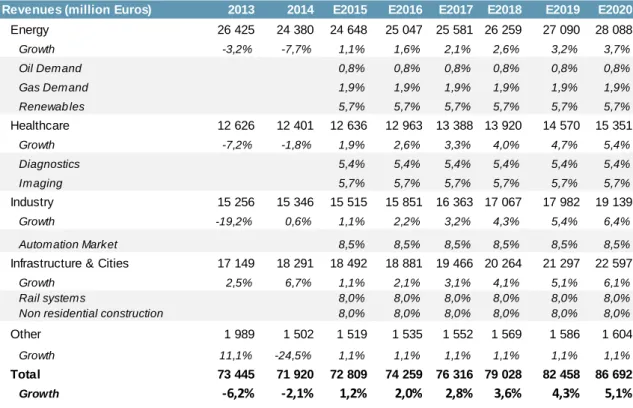
Revenues (million Euros) 2013 2014 E2015 E2016 E2017 E2018 E2019 E2020
Energy 26 425 24 380 24 648 25 047 25 581 26 259 27 090 28 088 Growth -3,2% -7,7% 1,1% 1,6% 2,1% 2,6% 3,2% 3,7% Oil Demand 0,8% 0,8% 0,8% 0,8% 0,8% 0,8% Gas Demand 1,9% 1,9% 1,9% 1,9% 1,9% 1,9% Renewab les 5,7% 5,7% 5,7% 5,7% 5,7% 5,7% Healthcare 12 626 12 401 12 636 12 963 13 388 13 920 14 570 15 351 Growth -7,2% -1,8% 1,9% 2,6% 3,3% 4,0% 4,7% 5,4% Diagnostics 5,4% 5,4% 5,4% 5,4% 5,4% 5,4% Imaging 5,7% 5,7% 5,7% 5,7% 5,7% 5,7% Industry 15 256 15 346 15 515 15 851 16 363 17 067 17 982 19 139 Growth -19,2% 0,6% 1,1% 2,2% 3,2% 4,3% 5,4% 6,4% Automation Market 8,5% 8,5% 8,5% 8,5% 8,5% 8,5%
Infrastructure & Cities 17 149 18 291 18 492 18 881 19 466 20 264 21 297 22 597
Growth 2,5% 6,7% 1,1% 2,1% 3,1% 4,1% 5,1% 6,1%
Rail systems 8,0% 8,0% 8,0% 8,0% 8,0% 8,0%
Non residential construction 8,0% 8,0% 8,0% 8,0% 8,0% 8,0%
Other 1 989 1 502 1 519 1 535 1 552 1 569 1 586 1 604
Growth 11,1% -24,5% 1,1% 1,1% 1,1% 1,1% 1,1% 1,1%
Total 73 445 71 920 72 809 74 259 76 316 79 028 82 458 86 692
Growth -6,2% -2,1% 1,2% 2,0% 2,8% 3,6% 4,3% 5,1%
28 5.2.2 Cost Structure and other Income
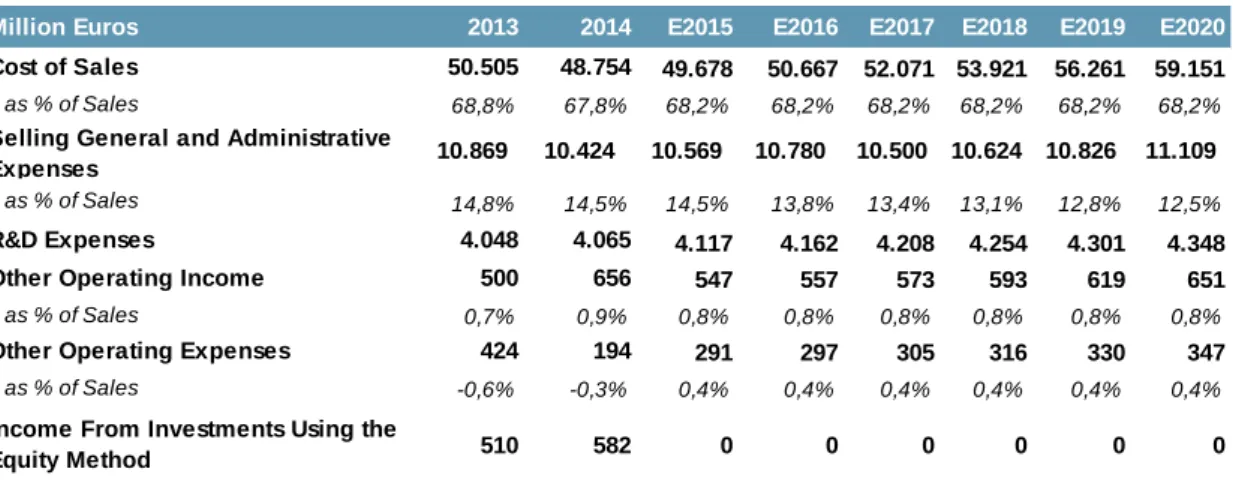
Cost of Sales (COGS)
The cost structure of Siemens consolidated is quite constant in general, the historical COGS as percentage of sales, is a clear example, where the values range between 66.1% and 69.2%.
Giving the constant structure, it was assumed that the average of the last three years would be a good representative of the future cost of sales. In addition, as it was mentioned in the macroeconomic analysis, the prices in real terms of aluminum and copper are not expected to differ much in the future and for that it will have little impact in the supply costs.
Selling General and Administrative Expenses
This type of expenses also followed a fairly constant weight of total sales, ranging from 14% to 17.6%.
The reasoning behind this forecast is similar to the one used above, where the value of 2015 is equal to the average of the last 3 years, although, it also considered the
company’s objective to decrease these costs by €1,000 million until 2016 and the economy of scale effects caused by the increase in sales.
R&D Expenses
This company follows an accounting policy where the Research & Development expenses are not capitalized until it is confirmed that there will be possible economic gains coming from it. For the forecasted period, the accounting policy will be kept since
Million Euros 2013 2014 E2015 E2016 E2017 E2018 E2019 E2020
Cost of Sales 50.505 48.754 49.678 50.667 52.071 53.921 56.261 59.151
as % of Sales 68,8% 67,8% 68,2% 68,2% 68,2% 68,2% 68,2% 68,2%
as % of Sales 14,8% 14,5% 14,5% 13,8% 13,4% 13,1% 12,8% 12,5%
R&D Expenses 4.048 4.065 4.117 4.162 4.208 4.254 4.301 4.348
Other Operating Income 500 656 547 557 573 593 619 651
as % of Sales 0,7% 0,9% 0,8% 0,8% 0,8% 0,8% 0,8% 0,8%
Other Operating Expenses 424 194 291 297 305 316 330 347
as % of Sales -0,6% -0,3% 0,4% 0,4% 0,4% 0,4% 0,4% 0,4%
10.826 11.109
0 0 0
Selling General and Administrative
Expenses 10.869 10.424 10.569 10.780 10.500 10.624
Income From Investments Using the
Equity Method 510 582 0 0 0
29
the levels of expenses have been constant in the last years as well as the value of Intangible Assets. In order to replicate these expenses for the following years, the average of the 3 years was used.
Other Operational Incomes and Expenses
The additional income and expenses related with operations concerns mostly impairments, sales of PPE and Intangible Assets, operating leases and legal and regulatory matters.
These operational expenses have been decreasing pronouncedly since 2007 although, like the operational income, they have stabilized in the last years. Considering this, the last 3 years average as percentage of sales was used as a driver to forecast these items.
Income from Non-consolidated Associates
These gains or losses have been somewhat unstable, ranging from gains of €582 million to losses of €1,946 million. For the sake of the reliability of this valuation, this income will be assumed as zero for the explicit period. Moreover, giving the non-recurring nature of this item, it is excluded from the calculation of free cash flow.
5.2.3 Investment Policy
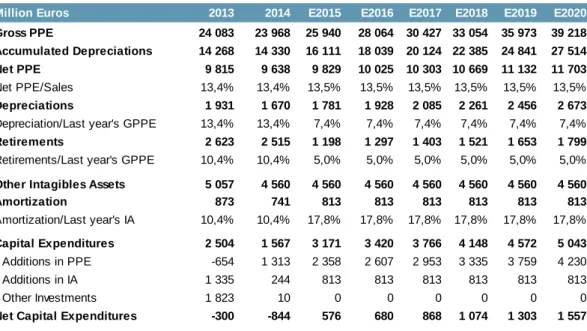
Million Euros 2013 2014 E2015 E2016 E2017 E2018 E2019 E2020
Gross PPE 24 083 23 968 25 940 28 064 30 427 33 054 35 973 39 218 Accumulated Depreciations 14 268 14 330 16 111 18 039 20 124 22 385 24 841 27 514 Net PPE 9 815 9 638 9 829 10 025 10 303 10 669 11 132 11 703
Net PPE/Sales 13,4% 13,4% 13,5% 13,5% 13,5% 13,5% 13,5% 13,5%
Depreciations 1 931 1 670 1 781 1 928 2 085 2 261 2 456 2 673
Depreciation/Last year's GPPE 13,4% 13,4% 7,4% 7,4% 7,4% 7,4% 7,4% 7,4%
Retirements 2 623 2 515 1 198 1 297 1 403 1 521 1 653 1 799
Retirements/Last year's GPPE 10,4% 10,4% 5,0% 5,0% 5,0% 5,0% 5,0% 5,0%
Other Intagibles Assets 5 057 4 560 4 560 4 560 4 560 4 560 4 560 4 560
Amortization 873 741 813 813 813 813 813 813 Amortization/Last year's IA 10,4% 10,4% 17,8% 17,8% 17,8% 17,8% 17,8% 17,8% Capital Expenditures 2 504 1 567 3 171 3 420 3 766 4 148 4 572 5 043 Additions in PPE -654 1 313 2 358 2 607 2 953 3 335 3 759 4 230 Additions in IA 1 335 244 813 813 813 813 813 813 Other Investments 1 823 10 0 0 0 0 0 0
Net Capital Expenditures -300 -844 576 680 868 1 074 1 303 1 557 Table 7: Investment Policy
30
This topic concerns every addition in PPE (Property, Plants and Equipment), Intangible assets and portfolio of businesses. As it was mentioned in the methodology, this
valuation will assume no portfolio adjustments. Regarding PPE, Siemens has gone through a reduction in the last 4 years where most of it was due to the disposal of obsolete assets. Adding to this, the net capital expenditures have been negative since 2008.
For the explicit period, it was considered that the continuation of this policy is unlikely, even more giving the projection of revenues. Then, the new investment policy will follow the trend of sales. In order to do that, it was used the ratio of Net PPE/Sales. The depreciation was determined by the last 3 years average of the ratio
Depreciation/Last year’s GPPE. Also, it was considered an annual amount of
retirements of 5%, using Retirements/ Last year’s GPPE. This value is lower than the company’s recent past since part of that value was composed by transfers to Assets Held for Disposal due the portfolio divestments.
Regarding intangible assets and the respective amortization, it was assumed that the additions minus amortization will equal zero. This assumption comes with the impossibility to determine when the company will be able capitalize any R&D
expenses. Adding to this is the fact that the amounts in intangible assets have remained stable which makes it a more reasonable assumption. Also, Goodwill will be maintained as it is, due to the no acquisitions assumption mentioned above, and no impairments will be recognized.
Finally, after all these assumptions, is possible to obtain the value of capital expenditures for each year, as it can be seen in the table.
5.2.4 Working Capital
This component represents the difference between the current assets and the current liabilities. These assets exclude any financial assets and excess cash. Siemens has been increasing its working capital needs, annually, from 2010 until now. The items used to determine it were: Trade Receivables, Inventories and Other Current Assets, on the side of assets, Accounts Payable and Other Current Liabilities on the side of liabilities.
31
The forecasting was done in percentage of sales, mainly because the items referred are all dependent of the volume of existing business, and also, since COGS driver happens to be sales there was no point in using it as a driver to Trade Payables or Inventories. Criteria used was the same as in the previous forecasts, the average of the last 3 years. In the end, the component that will be used in the valuation is the Net Working Capital, which is the difference between the Working Capital needs from one year to the next. By looking at the table, the values become positive after the first year which is caused by the revenue growth. The reduction in the first year is a consequence of the
normalization effect caused by the use of a 3 year average.
5.2.5 Taxes
When analyzing the consolidated results of Siemens it is possible to look at the annual value of taxes attributable to Net Income. Even though this is way more complex than that since the tax rates differ a lot from country to country, the calculation of the historical effective tax rate returns percentages very close to each other, around 30% (see Appendix 8.6). Then, it seems safe to admit that this component will continue
As % of Sales 2013 2014 E2015 E2016 E2017 E2018 E2019 E2020
Current Assets 43,2% 43,0% 42,4% 42,4% 42,4% 42,4% 42,4% 42,4%
Trade and other Receivables 20,2% 20,2% 20,0% 20,0% 20,0% 20,0% 20,0% 20,0%
Inventories 21,2% 21,0% 20,7% 20,7% 20,7% 20,7% 20,7% 20,7%
Other Operational Assets 1,8% 1,8% 1,7% 1,7% 1,7% 1,7% 1,7% 1,7%
Current Liabilities 37,2% 35,5% 36,3% 36,3% 36,3% 36,3% 36,3% 36,3%
Accounts Payable 10,3% 10,6% 10,4% 10,4% 10,4% 10,4% 10,4% 10,4%
Other Current Liabilities 26,8% 25,0% 25,9% 25,9% 25,9% 25,9% 25,9% 25,9%
Working Capital 6,0% 7,5% 6,1% 6,1% 6,1% 6,1% 6,1% 6,1%
Million Euros 2013 2014 E2015 E2016 E2017 E2018 E2019 E2020
Current Assets 31.703 30.923 30.885 31.500 32.372 33.522 34.978 36.774
Trade and other Receivables 14.853 14.526 14.528 14.817 15.228 15.769 16.453 17.298
Inventories 15.560 15.100 15.097 15.398 15.825 16.387 17.098 17.976
Other Operational Assets 1.290 1.297 1.259 1.285 1.320 1.367 1.426 1.500
Current Liabilities 27.300 25.548 26.428 26.954 27.701 28.685 29.930 31.467
Accounts Payable 7.599 7.594 7.565 7.715 7.929 8.211 8.567 9.007
Other Current Liabilities 19.701 17.954 18.863 19.239 19.772 20.474 21.363 22.460
Working Capital 4.403 5.375 4.457 4.546 4.672 4.838 5.048 5.307
Net Working Capital 570 972 -918 89 126 166 210 259
32
following the same trend. In order to come up with a tax rate for the next years, it was used the average of the last 3 years.
5.2.6 Debt
As it was said in the methodology section, the capital structure of Siemens will vary in market value terms. The fact that Siemens’s Debt is predominantly composed by bonds with fixed rates helped, since these traded securities have their market values available. Using Bloomberg, it was possible to extract the price of each bond that was issued. When multiplying the price of the bond for its respective carrying amount, the market value of a bond is obtained.
Table 9: Outstanding Bonds Composition
Source: Bloomberg
The other type of debt, bonds with floating rates, loans from banks and financial leases represent 13% of the total debt in book values. Giving this and the difficulty to find exact maturities and interest rates, these other types of debt were considered in book value terms.
Type Currency Amount (€) Issuance MaturityCarryig Amount (€) Price (€) Value (€) Yield Senior Unsecured USD 1 750 16/08/2006 17/10/2016 1 457 107,4 1 564 0,80% Senior Unsecured USD 500 16/03/2006 16/03/2016 425 104,6 445 0,58% Senior Unsecured EUR 2 000 20/02/2009 20/02/2017 2 122 109,2 2 318 0,12% Senior Unsecured EUR 1 600 11/06/2008 11/06/2018 1 839 117,0 2 151 0,22% Senior Unsecured USD 500 12/03/2013 12/03/2018 396 101,3 401 1,05% Senior Unsecured EUR 1 000 10/09/2012 10/03/2020 995 105,6 1 050 0,35% Senior Unsecured EUR 1 250 12/03/2013 12/03/2021 1 276 107,6 1 373 0,45% Senior Unsecured GBP 350 10/09/2012 10/09/2025 448 104,1 466 2,30% Senior Unsecured USD 1 750 16/08/2006 17/08/2026 1 843 128,5 2 368 3,12% Senior Unsecured EUR 1 000 12/03/2013 10/03/2028 996 122,1 1 216 1,03% Senior Unsecured USD 100 12/03/2013 12/03/2028 77 97,9 75 3,71% Senior Unsecured GBP 650 10/09/2012 10/09/2042 819 112,2 919 3,08% Senior Unsecured - With Warrants USD 1 500 16/02/2012 16/08/2017 1 158 112,0 1 297 -3,81% Senior Unsecured - With Warrants USD 1 500 16/02/2012 16/08/2019 1 140 116,6 1 329 -1,99% Subordinated, unsecured - Hybrid GBP 750 14/09/2006 14/09/2066 1 025 143,1 1 467 2,19% Subordinated, unsecured - Hybrid EUR 900 14/09/2006 14/09/2066 959 83,6 802 0,89%
Total 17 100 16 975 19 241
Million Euros Short-term Long-term Total Weight
Bonds with Floating Rate - 1 190 1 190 6% Bonds with Fixed Rate - 16 975 16 975 81% Loans from banks 773 968 1 741 8% Other financial indebtedess 826 85 911 4% Finance leases 21 108 129 1% Total 1 620 19 326 20 946
33
As it was said in the company presentation section, Siemens’s debt ratio has fluctuated in last 8 years where the cash variations have contributed a great deal (see Appendix 8.4). For the purpose of keeping the company structure consistent with the past, it was assumed that the debt value would grow with the total assets by maintaining a constant gross debt ratio, independently of the cash amounts.
The company has presented inconstant historical interest rates (interest expenses/Last year’s debt value), ranging from 14%, in 2009, to 4% in the last year. For the explicit period it was used the average of the last 4 years, considering that the recent fall in interest rates will not continue indeterminately, and by using information of the last 4 years it is expected to normalize possible future variations.
5.2.7 Financial Statements
In order to construct the forecasted financial statements it is necessary to go over items other than the ones mentioned above, even though they do not enter in the free cash flows.
The importance of having complete financial statements along the explicit period is concerned with the fact that it is the best way to check whether the assumptions made make sense or not. These items are presented in the Appendix 8.8.
Million Euros 2013 2014 E2015 E2016 E2017 E2018 E2019 E2020
Total Debt 20 452 20 948 20 814 20 770 21 062 21 396 21 783 22 232
Short-term and Current Maturities 1 945 1 620 2 952 2 946 2 988 3 035 3 090 3 154 Long-term 18 507 19 328 17 861 17 824 18 074 18 361 18 693 19 078 Debt/Assets 20% 20% 20% 20% 20% 20% 20% 20% Long-term Debt/Assets 18% 18% 17% 17% 17% 17% 17% 17% Cash 9 190 8 013 8 141 7 999 9 787 11 713 13 819 16 152 Net Debt 11 262 12 935 12 672 12 771 11 275 9 683 7 964 6 079 BV Debt Ratio 11% 12% 12% 12% 11% 9% 7% 5% Interest Expenses 784 764 1 350 1 341 1 338 1 357 1 379 1 403
Interest Expenses/Last year's Debt 3,8% 3,7% 6,4% 6,4% 6,4% 6,4% 6,4% 6,4%
Interest Coverage Ratio 6,8 8,8 4,2 4,3 4,8 5,3 5,9 6,5 Table 11: Debt Composition and Other Financial Information