Acknowledgement
I am extremely grateful to my parents and brother for all the support during my academic path until today. Without them this work would not have been possible. I would also like to thank Professor Alfredo Egídio dos Reis for all the support, precious suggestions and ideas for this work.
To Sara for all the patience during the last few months. To Tiago Campeã for trying to teach me the importance of typography. To all my friends, especially the eight who joined me during the last …ve years.
Abstract
We recover the classical actuarial risk model with a di¤usion component like in the model introduced by Dufresne and Gerber (1991). We just target the computation of the ruin probability in in…nite time by approximation, picking up some simple and classical methods, built for the basic or classical Cramér-Lundberg model, that can be adapted for the perturbed model in an easy way.
In particular, we consider the well-known methods by De Vylder, Dufresne & Gerber’s bounds approach, Beekman-Bowers’and the Tijms’ approximations. We further consider the adaptation of the Fourier/Laplace transforms method worked for instance by Lima et al. (2002).
With the help of several examples we attempt the accuracy of the approxim-ations, some light and fat tail distributions for the individual claim severity were used. We evaluate the ultimate ruin probability and separate the probability of ruin due to the introduction of the oscillating component.
Keywords: Perturbed risk model; di¤usion; ruin probability; ruin probability approximations; ruin probability by oscillation.
Resumo
Trabalhamos o modelo clássico de risco perturbado por difusão, em particular, o modelo introduzido por Dufresne and Gerber (1991). O objectivo é aproximar a probabilidade de ruína em tempo in…nito para este modelo usando algumas aprox-imações simples e clássicas, originalmente apresentadas para o modelo clássico de Cramér-Lundberg e que são facilmente adaptáveis para este modelo.
Em particular é trabalhada a aproximação de De Vylder, o método de Dufresne & Gerber que permite a construção de limites inferiores e superiores para a probab-ilidade de ruína, a aproximação de Beekman-Bowers e a aproximação de Tijms. É ainda considerada uma adaptação do método das transformadas de Fourier/Laplace, usado por exemplo em Lima et al. (2002).
Recorrendo a vários exemplos é testada a precisão das aproximações, usando distribuições de cauda leve e de cauda pesada. É calculada a probabilidade de ruína em tempo in…nito e separada a probabilidade de ruína devida à introdução da componente oscilatória.
Palavras-chave: Modelo de risco perturbado; difusão; probabilidade de ruína; aproximações à probabilidade de ruína; ruína causada por oscilação.
Contents
Introduction 1
1 The Perturbed Model 3
1.1 Model description . . . 3
1.2 Probability of ruin . . . 4
1.3 The adjustment coe¢ cient and a simple upper bound . . . 6
1.4 Exact ruin probabilities for mixture of exponentials . . . 6
1.5 Maximal aggregate loss . . . 8
1.6 Asymptotic results . . . 11
2 Approximation methods 12 2.1 De Vylder’s approximation . . . 12
2.2 Dufrene & Gerber’s upper and lower bounds . . . 13
2.3 Beekman-Bowers’approximation . . . 15
2.4 Tijms’approximation . . . 17
2.5 Fourier transform and ruin . . . 18
2.5.1 Fourier transform . . . 18
2.5.2 Applying the inversion formula . . . 20
3 Numerical illustrations 22 3.1 Exponential distribution . . . 22 3.2 Mixture of exponentials . . . 23 3.3 Gamma distribution . . . 26 3.4 Pareto distribution . . . 29 Conclusions 32
B Convolutions 35
C Laplace transform 37
D Renewal theory 39
List of Tables
3.1 Exact …gures, Exponential. . . 23
3.2 Beekman-Bowers’, Tijms’and Fourier methods, Exponential. . . 24
3.3 Fourier method for d(u) and s(u), Exponential. . . 24
3.4 Exact …gures, Mixture of Exponentials. . . 25
3.5 De Vylder’s, Beekman-Bowers’and Tijms’methods, Mixture of Ex-ponentials. . . 26
3.6 Fourier method, Mixture of Exponentials. . . 27
3.7 Fourier method for d(u) and s(u), Mixture of Exponentials. . . 27
3.8 Dufresne & Gerber’s Bounds, De Vylder’s, Beekman-Bowers’, Tijms’ and Fourier Methods, Gamma. . . 28
3.9 De Vylder’s and Fourier methods for d(u) and s(u), Gamma. . . . 29
3.10 Dufresne & Gerber’s Bounds, De Vylder’s and Beekman-Bowers’meth-ods, Pareto. . . 30
3.11 Fourier method for d(u) and s(u), Pareto. . . 31
List of Figures
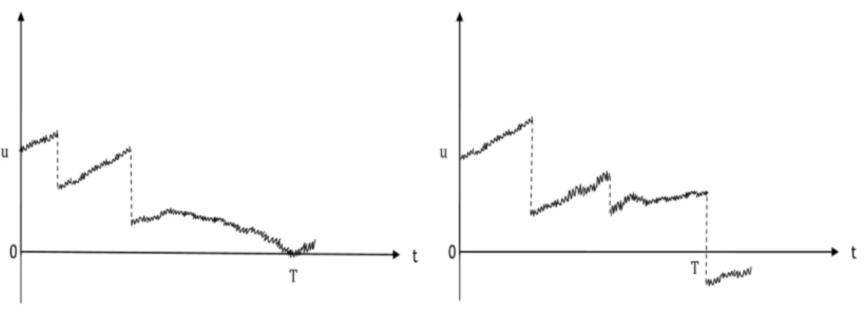
1.1 The two types of ruin, due to oscillation and because of a claim. . . . 4Introduction
The so called risk models in actuarial science are much focused in modelling the surplus process of the insurance business. In these models, like in any other math-ematical models we have to make simpli…cations of the real world. One simpli…cation that is made in the classical risk model is that no other factors than the received premiums and the paid claims a¤ect the surplus. The object of study in this work is the perturbed model introduced in actuarial science by Dufresne and Gerber (1991). By adding a di¤usion component to the classical surplus process, it allows to consider other factors to a¤ect the surplus such as the uncertainty of the premium income, changes in the number of clients, ‡uctuations of the interest rate or deviations in the claims payouts, without discarding all the other assumptions.
The aim of this work is to obtain approximations for the probability of the surplus process becoming negative in in…nite time horizon (ultimate ruin). Closed ruin probability formulae are known in some special cases and so we aim to approximate this probability using a variety of di¤erent methods. In this work we consider some simple and well known methods that are applied in the classical risk model and we translate them to the perturbed model.
The work that follows in the next pages can be seen as a sequel of previous works like Silva (2006) and Jacinto (2008). The …rst author adapted to the perturbed model the De Vylder’s method and the Dufresne & Gerber’s upper and lower bounds. The latter presented some numerical illustrations of these methods and a …rst try to adapt the Beekman-Bowers’approximation.
In this dissertation we …rst present the perturbed model, we review and correct the methods adapted by Silva (2006) and we try to improve the Beekman-Bowers’ approximation presented by Jacinto (2008). We add to these methods the Tijms’ approximation and also one possible application of the Fourier transform to obtain ruin probabilities in this model.
to evaluate the accuracy of the di¤erent methods by comparing the results with exact ones available, or with the upper and lower bounds. In addition to the approximate …gures of the ultimate ruin probability, we present also …gures for the ultimate ruin probability due to the di¤usion component and the weight that this form of ruin has to the total ruin probability in each of the examples.
It is assumed during this work that the reader is familiar with ruin theory and specially with the classical continuous time model, also known as the Cramér-Lundberg model. Good …rst references are Dickson (2005), Gerber (1979), Kaas et al : (2008) or even Klugman et al. (2008).
1
The Perturbed Model
In this chapter we introduce the model as presented by Dufresne and Gerber (1991). We de…ne the perturbed surplus process, the probability of ruin and its decompos-ition, the adjustment coe¢ cient and some particular cases where it is possible to calculate the exact ruin probability. We also de…ne the process of aggregate loss, the maximal aggregate loss and also one possible decomposition for it. Last but not least, asymptotic results for the ruin probabilities are presented. Proofs of the theorems, when not presented can be seen on that paper.
1.1
Model description
The perturbed surplus process at time t is de…ned as:
V (t) = U (t) + W (t),
U (t) = u + ct S(t); t 0,
where U (t) de…nes the well known classical surplus process, c is the rate at which premiums are received, u = V (0) = U (0) is the initial surplus, S(t) = PN (t)i=0 Xi,
X0 0 are the aggregate claims up to time t, N (t) is the number of claims
re-ceived up to time t, Xi is the i-th individual claim, W (t) is the di¤usion component
and 2
the variance parameter. fW (t); t 0g is a standard Wiener process (or Brownian Motion), fN(t); t 0g is a Poisson process with parameter and fXig1i=1
is a sequence of i:i:d: random variables, independent from fN(t)g with common distribution function P (:) with P (0) = 0 and pk= E[Xk]. The corresponding
dens-ity function is denoted as p(:). We assume that fS(t)g and fW (t)g are independent. We also assume that c = (1 + ) p1, where > 0 is the premium loading coe¢ cient.
The di¤usion component introduces an extra source of uncertainty to the classical model due to its oscillating nature and so the process V (t) becomes more uncertain than U (t). For more details about the Weiner process and the moments of V (t), please see Appendix A.
1.2
Probability of ruin
De…nition 1 Let T = inf ft : t 0 and V (t) 0g, be the moment of ruin, with the assumption that T = 1 if V (t) > 0, 8t:
De…nition 2 The probability of ultimate ruin from initial surplus u is
(u) = Pr(T <1jV (0) = u) = d(u) + s(u)
where d(u) = Pr(T <1 and V (T ) = 0 jV (0) = u) is the probability of ruin caused
by oscillation and s(u) = Pr(T < 1 and V (T ) < 0 jV (0) = u) is the probability
that ruin occurs due to a claim.
The survival probability is denoted as (u) = 1 (u). Due to the oscillating nature of the process we have that d(0) = (0) = 1 (see Appendix E). In Dufresne and Gerber (1991) important defective renewal equations for (u), (u), d(u)and
s(u) are derived.
Figure 1.1: The two types of ruin, due to oscillation and because of a claim.
Theorem 1 The survival probability for the process V (t) obeys to the following defective renewal equation:
(u) = qH1(u) + (1 q)
Z u 0
were q = 1 c p1 , q = 1+ and h1 h2(:) is the convolution of the following
density functions, with the respective distribution functions denoted H1(:) and H2(:),
h1(x) = e x, x > 0
h2(x) = p11[1 P (x)] , x > 0
= 2c= 2.
Equation (1:1) has some components that are well known from the classical model given by U (t). The expression for q is the survival probability with no initial reserve (u = 0) and h2(:) is the density function of the individual records from the
aggregate loss.
Theorem 2 The probability of ruin caused by oscillation and by claim, for the pro-cess V (t), obey to the following defective renewal equations, respectively:
d(u) = 1 H1(u) + (1 q)
Z u 0
d(u x)h1 h2(x)dx, u 0, (1.2) s(u) = (1 q) [H1(u) H1 H2(u)] +
+ (1 q) Z u
0
s(u x)h1 h2(x)dx, u 0, (1.3)
where q, H1(:) and H2(:) are the same as de…ned above.
Theorem 3 The ruin probability for the process V (t) obeys to the following defective renewal equation:
(u) = q [1 H1(u)] + (1 q) [1 H1 H2(u)] + (1.4)
+ (1 q) Z u
0
(u x)h1 h2(x)dx, u 0,
where q, H1(:) and H2(:) are the same as de…ned above.
Proof. Using the relation, (u) = 1 (u)in (1:1) or summing (1:2) with (1:3). These equations will have an important role in the approximations presented in the next chapters. For a brief idea about renewal equations and renewal theory, please see Appendix D.
1.3
The adjustment coe¢ cient and a simple upper bound
Using a martingale argument, Dufresne and Gerber (1991) de…ned the adjustment coe¢ cient and an upper bound similar to Lundberg’s inequality. The adjustment coe¢ cient plays an important role in the asymptotic formulas for the ruin probab-ilities, which also happens in the classical model. In what follows we assume that the moment generating function of the claim amount distribution, MX(s) = E[esX],
exists for 1 < s < and that lims! MX(s) = +1.
De…nition 3 The adjustment coe¢ cient R is the only positive root of the equation: MX(R) +
2
2 R
2
= + cR; r < (1.5)
We can see that the equation has only one positive root, letting h(r) = rc MX(r) + 2 2r 2 ) h(0) = 0. h0(r) = c MX0 (r) 2r ) h0(0) = c p1 > 0,
by the hypotheses of the model. h00(r) = MX00(r) 2 = E[X2erX] 2 < 0.
So h(r) is concave and as limr! h(r) = 1 ) the equation h(r) = 0 has two roots, one is r = 0 and the other is the positive root R.
With this result it is also possible to derive a simple upper bound for the ruin probability.
Theorem 4
(u) < e Ru; u > 0
where R is the adjustment coe¢ cient and u is the initial reserve.
1.4
Exact ruin probabilities for mixture of exponentials
As in the classical model, the exact ruin probability can be calculated when the claim amount distribution is exponential or mixture of exponentials.
Theorem 5 If the claim amount distribution has probability density function of the form p(x) = n X i=1 Ai ie ix; with n X i=1 Ai = 1 f or x > 0 (1.6)
then the exact ultimate ruin probability must be of the form (u) = n+1 X k=1 Cke rku; u 0 (1.7) where Ch = n Y i=1 rh i i n+1 Y k=1 k6=h rk rh rk ; f or h = 1; : : : ; n + 1 (1.8)
with Pn+1h=1Ch = 1 and r1;: : : ; rn+1 being the solutions of the equation n X i=1 Ai i r + 2 2 r = c (1.9)
Of course that if n = 1, we have the case where the claim size distribution is exponential with parameter . Under the same conditions it is also possible to obtain the exact ruin probability caused by oscillation.
Theorem 6 If the claim amount distribution has probability density function of the form (1:6), then the exact ruin probability by oscillation must be of the form
d(u) = n+1 X k=1 Ckde rku; u 0 (1.10) with Chd= rh q Ch = Qn i=1(rh i) Qn k=1;k6=h(rh rk) ; f or h = 1; : : : ; n + 1 (1.11) where r1;: : : ; rn+1 are the solutions of equation (1:9).
The probability of ruin caused by a claim can be simply calculated using the relation s(u) = (u) d(u). This decomposition can allow us to see the
contribu-tion of claims and oscillacontribu-tions to the occurrence of ruin. It is expectable that under the same perturbation by di¤usion (same ), the weight of the perturbation to the occurrence of ruin will be lower in a heavy tail distribution than in a light one.
1.5
Maximal aggregate loss
Considering the process V (t), we can construct the process of aggregate loss at time t, fL(t); t 0g:
L(t) = S(t) ct W (t), V (t) = u L(t) (1.12)
and we can de…ne the maximal aggregate loss,
De…nition 4 Let fL(t); t 0g be the process of aggregate loss, (1:12), then the maximal aggregate loss is the random variable L such that L = maxfL(t); t 0g:
We can express the survival probability in terms of L. As L(0) = 0 ) L 0,
Pr[L u] = Pr[L(t) u;8t 0] = Pr[S(t) ct W (t) u;8t 0] = Pr[V (t) 0;8t 0] = (u)
This way we can see that the survival probability is the distribution function of the random variable L. Contrary to the classical model, (u) does not have a mass point at zero, because Pr[L 0] = (0) = 0.
Dufresne and Gerber (1991) decomposed the maximal aggregate loss random variable into two kinds of "record highs". Letting M be the number of records of the process fL(t)g that are caused by claims and letting t1; : : : ; tM denote the times
when these claims occur with t0 = 0 and tM +1= +1, we can de…ne:
L(1)i = maxfL(t); t < ti+1g L(ti) f or i = 0; 1; : : : ; M
and
L(2)i = L(ti) L(ti 1) L (1)
i 1 f or i = 1; : : : ; M
where maxfL(t); t < ti+1g is the record due to the Wiener process that occurs before
the time ti+1. The random variables L (1)
i and L (2)
i represent the amounts that result
Figure 1.2: Decomposition of the maximal aggregate loss.
to oscillation and a claim, respectively, as it can be seen in …gure 1.2. These two types of random variables allow us to write the maximal aggregate loss as:
L = L(1)0 + L(1)1 + L(2)1 + : : : + L(1)M + L(2)M = L(1)0 +
M
X
i=1
L(1)i + L(2)i (1.13)
Note that L = L(1)0 if M = 0. The main idea behind this decomposition is that a certain record is simply the sum of the di¤erences between successive records until we obtain the "maximal record".
Theorem 7 fL(1)i gi=0;:::;M and fL (2)
i gi=1;:::;M are two sequences of independent and
identically distributed random variables with common probability density functions h1(x) and h2(x), respectively and also independent from M . So the distribution
functions of each L(1)i and L(2)i are,
Pr[L(1)i x] = H1(x) = 1 e x; x 0
Pr[L(2)i x] = H2(x) = p11
Z x 0
[1 P (y)] dy; x 0
Theorem 8 The random variable M is geometrically distributed, P [M = m] = q(1 q)m f or m = 0; 1; : : :
where q represents the probability that there are no record highs that are caused by a claim. This implies that (u) is a compound geometric distribution,
(u) =
1
X
m=0
q(1 q)mH1(m+1) H2m(u) (1.14)
where q, H1(:) and H2(:) are the same as de…ned above.
The convolution formula (1:14) generalizes a similar result in the classical model. Theoretically (1:14) can allow us to calculate the ruin probability but in practice this is often impossible due to the calculation of the convolutions of H1(:)and H2(:)with
themselves and the convolution between them. However, this convolution formula is the base for one of the approximation methods presented below.
We can calculate the moments of L, if they exist. The expected value and vari-ance were easily deducted by Jacinto (2008) considering that L = L(1)0 +
PM i=1 L (1) i + L (2) i is a compound distribution,
E[L] = E[L(1)0 ] + E[M ] E[L(1)i ] + E[L(2)i ]
V ar[L] = V ar[L(1)0 ] + E[M ] V ar[L(1)i ] + V ar[L(2)i ] + V ar[M ] E[L(1)i ] + E[L(2)i ]
2
Noting that
E[L(1)i ] = 1; V ar[L(1)i ] = 12; E[L
(2)k i ] = pk+1 (k+1)p1; V ar[L (2) i ] = p3 3p1 p2 2p1 2 And that
E[M ] = 1 qq and V ar[M ] = 1 qq2
Using the fact that q = 1 c p1 and = 2c2 we arrive to the following expressions,
E[L] = 2 2c + p1 2 2c + p2 2p1 c 1 cp1 (1.15) V ar[L] = 4 4c2 + p1 2 2c + p2 2p1 2 c 1 cp1 2 + p1 4 4c2 p2 2 4p2 1 + p3 3p1 c 1 cp1 (1.16)
Formulas (1:15) and (1:16) allow us to obtain this two moments in a easy way, using only values that are known from the beginning, if they exist. To obtain high-order moments we can use the moment generating function.
Theorem 9
ML(s) =
s (c p1)
+ cs ( s) MX(s)
(1.17)
Proof. See Appendix E.
1.6
Asymptotic results
The three defective renewal equations (1:2), (1:3) and (1:4) have a possible asymp-totic solution if we apply renewal theory techniques such as the ones presented in Appendix D. The solutions for the ruin probabilities demand the existence of the adjustment coe¢ cient and so we can only consider its use when the moment gener-ating function of X exists. These asymptotic solutions will be the base for one of the approximations presented below.
Theorem 10 If the adjustment coe¢ cient, R, exists, then as u ! 1 we have,
d(u) Cde Ru (1.18) s(u) Cse Ru (1.19) (u) Ce Ru (1.20) where, Cd= R1 0 e Rx[1 H 1(x)] dx (1 q)R01xeRxh 1 h2(x)dx Cs = R1 0 e Rx(1 q) [H 1(x) H1 H2(x)] dx (1 q)R01xeRxh 1 h2(x)dx and C = Cd+ Cs= R1 0 e Rx[q [1 H 1(x)] + (1 q) [1 H1 H2(x)]] (1 q)R01xeRxh 1 h2(x)dx
2
Approximation methods
2.1
De Vylder’s approximation
The main idea behind this approximation is to use the existence of a closed formula for the ruin probability when the individual claim amount distribution is expo-nential. This simple and practical approximation was originally proposed for the classical model by De Vylder (1978) where he replaces the original surplus process, U (t), by another one, let’s say, U (t) = u + c t S (t), matching the …rst three moments. This new process is characterized by the fact that S (t) is a compound Poisson distribution with parameter and the claim amount distribution is expo-nential with parameter . The third parameter that characterize the process is c , the new rate at which premiums are received. Equating the moments of the two processes we can …nd the expressions for the new parameters.
In the context of the perturbed model, a …rst adaptation of this approximation can be seen in Silva (2006) and some numerical illustrations can be seen at Jacinto (2008). The idea is similar to the original approximation but in the perturbed model we have an extra parameter, 2. Considering the process V (t) = U (t) + W (t), we can …nd the parameters , , c and 2 by equating the corresponding four central moments of V (t) and V (t). The moments of the process V (t) can be seen in Appendix A and as the …rst four raw moments of the exponential distribution are 1, 22,
6
3 and
24
4, the system to be solved is: 8 > > > > > > > < > > > > > > > : u + ct tp1 = u + c t t1 2t + tp 2 = 2t + t22 tp3 = t 63 tp4+ 3 2t2p22 + 6 t2p2 2+ 3 4t2 = t244 + 3 2t2 2 2 2 + 6 t2 2 2 2+ 3 4t2
Which leads to the following solution,
= 4p3 p4; = 32 p4 3 3p3 4; c = 8 p3 3 3p2 4 + c p1; 2 = 2+ p 2 4 p2 3 3p4.
As we can see by the …nal expressions of the parameters this method only requires the existence of the …rst four raw moments of the original claim amount distribution, which is not very restrictive when comparing it with more complex methods.
Having this parameters we can now apply formulas (1:7) and (1:8) in order to obtain the approximation, DV(u), given by,
DV(u) = C1e r1 + C2e r2; C1 = r1 r1r2r2; C2 = r2 r2r1r1 ,
where r1 and r2 are the solutions of the following equation 2
2 r + r = c .
With this method we can also obtain a simple approximation to the ruin probability due to oscillation, d(u) . Denoting the approximation as d;DV(u) and applying formulas (1:10) and (1:11), we obtain,
d;DV(u) = C1de r1 + C2de r2; C1d= qr1 C1; C d
2 = qr2 C2 ,
where r1 and r2 are the same as for the case of DV(u)but now q and are given
by,
q = 1 c 1; = 2 c 2
The approximation to the ruin probability due to a claim can be obtained simply using s;DV(u) = DV(u) d;DV(u).
2.2
Dufrene & Gerber’s upper and lower bounds
Since that the direct calculation of the ruin probability through formula (1:14) is most of the times impossible to obtain due to the calculation of the convolutions, Silva (2006) proposed a method to obtain bounds for the ruin probability that generalizes another one proposed for the classical model by Dufresne and Gerber (1989). The original method is based on de…ning appropriate discrete distributions to replace on the classical convolution formula for the survival probability and then, using the fact that (u) is a compound geometric distribution, apply the well know
recursive Panjer’s formula proposed by Panjer (1981). For the perturbed model we can use a similar method now based on formula (1:14). With this method we can obtain an upper and lower bound to the ruin probability because we use two types of discretization.
Following the methods by Dufresne and Gerber (1989), Silva (2006) starts by de…ning discrete random variables based on the decomposition of the maximal ag-gregate loss, Lj = Lj;(1)0 + M X i=1 Lj;(1)i + Lj;(2)i , with Lj = Lj;(1)0 if M = 0 and j = l; u with Ll;(k)i = # " L(k)i # # # (0; 1) Lu;(k)i = # " L(k)i + # # # # (0; 1)
for fk = 1; i = 0; :::; Mg and for fk = 2; i = 1; :::; Mg. [x] represents the integer part of x.
Thus the idea is to round the summands in (1:13) to the next lower multiple of # which gives Ll and to the next higher multiple of #, which gives Lu. Clearly,
Ll L Lu which implies that
Pr(Ll u) (u) Pr(Lu u)
This discretization of L implies that the probability functions of the discrete random variables Ll;(1)i ; Ll;(2)i ; Lu;(1)i and Lu;(2)i are, respectively:
hl1;k = Pr Ll;(1)i = k# = H1(k# + #) H1(k#), k = 0; 1; :::
hl2;k = Pr Ll;(2)i = k# = H2(k# + #) H2(k#), k = 0; 1; ::: ,
hu1;k = Pr Lu;(1)i = k# = H1(k#) H1(k# #), k = 1; 2; :::
Where H1(:) and H2(:) are the same as de…ned above. Note that hl1;k is the
prob-ability of Ll;(1)i being equal to k#, i.e., that L(1)i is between k# and k# + #. Similar interpretations can be done to hl
2;k; hu1;k and hu2;k:
If we write the probability functions of Ll and Lu as
fkj = Pr Lj = k# , k = 0; 1; ::: for j = l; u. we have then the following bounds for (:)
1 m 1X k=0 fkl (m#) 1 m X k=0 fku, m = 0; 1; :::u=#, u = 0; 1; ::
The calculation of these bounds is possible using the Panjer’s recursion formula for the compound geometric distribution (see Panjer (1981)). We arrive then to the following distributions of fl
k and fku (please see Silva (2006) for further details),
fkl = 8 > > > > < > > > > : qhl 1;0 1 (1 q)hl 1;0hl2;0, k = 0 1 1 (1 q)hl 1;0hl2;0 2 4 qh l 1;k + (1 q) h l 1;0 Pk j=1f l k jh l 2;j + (1 q)Pki=1Pk ij=0fl k i jhl1;ihl2;j 3 5 , k = 1; 2; ::: and fku = 8 > > > < > > > : 0, k = 0 qhu 1;1, k = 1 qhu 1;k+ (1 q) Pk 1 i=1 Pk i j=1f u k i jhu1;ihu2;j, k = 2; 3; :::
This method is very useful to test the accuracy of other approximations for the cases where we do not have exact results for the ruin probability.
2.3
Beekman-Bowers’approximation
This approximation is a modi…cation of an approximation presented for the clas-sical model by Beekman (1969) and the main idea is to use a gamma distribution in the renewal equation for the survival probability. In the classical model this equation is given by (u) = (0) + (0)R0u (u x)[1 P (x)]p
1 dx, please see for in-stance Dickson (2005) for further details. What the Beekman-Bowers’approxima-tion does in this case is to approximate the survival probability by BB(u) = (0)+
(0)R0u ( )x 1e xdx. The integral in this expression represents now a cumulative distribution function of a gamma( ; ) at point u. The parameters of this gamma are chosen by matching the moments of the r.v. L with the moments of BB(:).
To adapt this approximation to the perturbed model, instead of replacing the whole integral by a gamma distribution in (1:1), as presented by Jacinto (2008), we start with the idea of replacing the convolution h2(:) by a cumulative
distribu-tion funcdistribu-tion of a gamma( ; ). Using the properties of convoludistribu-tions and de…ning H3(u) =
Ru 0 ( )x
1e xdx, we can write the approximation as,
(u) = qH1(u) + (1 q)h1 h2(u)
) BB(u) = qH1(u) + (1 q)h1 H3(u) (2.1)
In order to obtain and , we can still use the relation between L and (:). We can …nd the moments of this new approximation applying the Laplace transform on (2:1) and equating them with the moments of L. The de…nition and some useful properties of the Laplace transform can be seen in Appendix C.
Taking Laplace transforms on (2:1) we obtain,
BB(s) = qh1(s) + (1 q)h1(s)h3(s) where BB(s) = R1 0 e syd BB(y); h1(s) = R1 0 e syh 1(y)dy; h3(s) = R1 0 e sydH 3(y)
Note that the Laplace transform here is calculated using the density functions, in order to be possible to calculate the moments. As h1(y) is the density function of
an exponential distribution with parameter , the corresponding Laplace transform is given by h1(s) = +s. For the gamma density, the Laplace transform is given by
h3(s) = +s . So BB(s) can be written as,
BB(s) = q
+ s + (1 q) + s + s (2.2)
0we arrive to, d dsjs=0 BB (s) = q (1 q) + d2 ds2 js=0 BB (s) = 2q2 + (1 q)2 2 + 2 + (1 + ) 2 2 2
Using the relation V ar[L] = E[L2] E2[L] and equating these two new expressions
with the expressions for E[ L] and E[L2](see (1:15) and (1:16)) we can …nd and
and approximate the ruin probability using (2:1). This leads us to the idea that this approximation might not be as good as the De Vylders’s approximation since there we are matching four moments and here we are only matching two.
2.4
Tijms’approximation
Tijms (1994) proposed an approximation that takes advantage of the asymptotic behaviour for large u and smooth it for small u. This approximation was originally presented in the context of queuing theory but it has been adapted by many authors for the ruin probability in the classical model. See for instance Dickson (2005) or Klugman et al. (2008).
The idea is to add an exponential term to (1:20) in order to improve the accuracy for small u. We de…ne the approximation as
T(u) = Ce Ru+ Ae Su; u 0
where A is chosen in such a way that the probability with no initial reserve matches the exact probability, i.e., (0) = T(0). As (0) = 1, we have A = (1 C). Also, as (:) is the survival function of L, S is chosen in order that R01 T(u)du = E[L].
So we have, E[L] = C R + (1 C) S , S = R (1 C) RE[L] C
This approximation can only be used for the cases where the moment generating function of X exists, in order to exist the adjustment coe¢ cient. It is an approx-imation easy to set and understand, the major problem is the computation of C.
The approximation is likely to produce good results if the choice of S through the expected value of L is enough to smooth the asymptotic result for small values of u:
2.5
Fourier transform and ruin
This section is inspired on a previous work by Lima et al. (2002) where the authors used the Fourier transform to obtain ruin probabilities in the classical model. Here we present the transform, some properties, the key results used by them and adapt the methodology to the perturbed model.
We must note that this method is not an approximation like the others presented above. Ideally, with the expressions developed here we should be able to compute exact ruin probabilities but we obtain di¤erences to the exact values due to the accumulation of numerical errors in the computations and not due to the lack of suitability of the method to a particular claim amount distribution.
2.5.1 Fourier transform
The Fourier transform of a continuous function, f (x), de…ned for x 0 whose integral exists for all x > 0 is de…ned as
f (x)(s) =
Z +1 0
eisxf (x)dx
where i2 = 1. We note that if f (:) is a density function then,
f (:)(s) is the
corresponding characteristic function. The transform has some useful properties that are used in this work. They are presented below and the proofs can be seen for instance at Poularikas (1996).
Property 1 Let f (:) and g(:) be de…ned on <+0 as above and h(x) = af (x) + bg(x), where a and b are two constants. Then
Property 2 Let F (:) be de…ned on <+0 as above, limx!1F (x) = 1 and f (x) = F0(x). Then 1 F (x)(s) = i(1 F (0)) s i s f (x)(s)
Property 3 Let ffj(:)gnj=1be functions de…ned on <+0 as above, and let h(:) be the
n-th convoluted function, h(x) = f1 f2 fn(x). Then
h(x)(s) = n
Y
i=1
fi(x)(s)
Another interesting fact about the Fourier transform is that it can always be splitted into two parts. The real part and the complex part, which can be veri…ed through Euler’s formula, eix = cos(x) + i sin(x). We can then write,
f (x)(s) = r f (x)(s) + i c f (x)(s) = Z +1 0 cos(sx)f (x)dx + i Z +1 0 sin(sx)f (x)dx
where rf (x)(s) represents the real part of the transform and cf (x)(s) the complex part. Also, considering the Fourier cosine transform,
'(s) = Z 1
0
cos(sx)f (x)dx
we can recover the integral of the original function with the inverse transform: Z x 0 f (y)dy = 2 Z 1 0 sin(xs) s '(s)ds
where f (x) is a continuous non-negative function de…ned on <+, whose integral exists for all x > 0. From this well known result we can write the following theorem.
Theorem 11 Let f (x) be a continuous non-negative function de…ned on <+0 whose integral exists for all x > 0, and f (x) = F0(x). Then,
F (x) = F (0) + 2 Z 1 0 sin(xs) s r f (x)(s)ds (2.3)
The proof of this result can be seen at Poularikas (1996), for instance. The fact that we can obtain the cosine transform from the Fourier transform, which
corresponds to the real part of the transform, makes (2:3) a very useful method to obtain ruin probabilities. The major problem when applying this method is that the integrand function in (2:3) can be a rapidly oscillating function, which leads to a series of numerical problems when computing the integral. Lima et al. (2002) solved this problem using what they called the dicotomic approach algorithm, which revealed extremely good results at the time. In our case we used the Mathematica package to invert the Fourier transform, which was capable of reproduce most of the original …gures.
2.5.2 Applying the inversion formula
In order to use formula (2:3) to obtain ruin probabilities we have to obtain …rst expressions for 0d(u), 0s(u) and 0(u). Starting from (1:2), (1:3) and (1:4) and using the Leibniz’s di¤erentiation rule we obtain respectively,
0
d(u) = h1(u) + (1 q)h1 h2(u) + (1 q)
Z u 0
0
d(u x)h1 h2(x)dx 0
s(u) = (1 q)h1(u) (1 q)h1 h2(u) + (1 q)
Z u 0 0 s(u x)h1 h2(x)dx 0(u) = qh 1(u) + (1 q) Z u 0 0(u x)h 1 h2(x)dx
Applying the Fourier transform to these expressions we obtain, using Properties 1 and 3,
0
d(u)(s) =
h1(u)(s) + (1 q) h1(u)(s) h2(u)(s) 1 (1 q) h
1(u)(s) h2(u)(s) 0
s(u)(s) =
(1 q) h1(u)(s) (1 q) h1(u)(s) h2(u)(s) 1 (1 q) h1(u)(s) h2(u)(s)
0(u)(s) =
q h1(u)(s)
These expressions can be rearranged according to h1(u)(s) =
r
h1(u)(s) + i
c
h1(u), and using Property 2, h2(u)(s) = spi
1 p(u)(s) sp1 i = c p(u)(s) sp1 + (1 r p(u)(s)) sp1 i, we obtain: (1 q) h1(u)(s) h2(u)(s) = 1 q sp1 r h1(u)(s) c p(u)(s) c h1(u)(s) + c h1(u)(s) r p(u)(s) +i1 q sp1 r h1(u)(s) r h1(u)(s) r p(u)(s) + c h1(u)(s) c p(u)(s) = 1 q sp1 J + i1 q sp1 I
Where J and I correspond to the expressions in brackets. This leads to,
0 d(u)(s) = r h1(u)(s) i c h1(u)+ 1 q sp1J + i 1 q sp1I 1 1 qsp 1J i 1 q sp1I (2.4) 0 s(u)(s) = (1 q) rh1(u)(s) + i (1 q) ch1(u) 1 qsp 1J i 1 q sp1I 1 1 qsp 1J i 1 q sp1I (2.5) 0(u)(s) = q rh1(u)(s) iq ch1(u) 1 1 qsp 1J i 1 q sp1I (2.6)
We must now split the transforms into the real and the complex parts in order to apply (2:3) and obtain expressions of the following type,
(u) = (0) + 2 Z +1 0 sin(us) s r 0(u)(s)ds If we do A = q rh1(u)(s) B = q ch1(u) C = 1 1 qsp 1J D = 1 q sp1I we can write (2:6) as,
0(u)(s) =
A + iB
C iD =
AC BD + i(BC + AD) C2+ D2
and (2:3) becomes, in this case,
F(u) = (0) + 2 Z +1 0 sin(us) s AC BD C2 + D2 ds (2.7)
We present only the case for F(u), but similar reasonings can be done to obtain expressions to d;F(u)and s;F(u), starting from (2:4) and (2:5), respectively.
3
Numerical illustrations
For purposes of testing the accuracy of the di¤erent methods we present here some numerical examples. In all of them we are going to assume that the premium rate is equal to c = 2, every individual claim amount distribution has mean p1 = 1, the
Poisson parameter is = 1 and the volatility is also = 1. This leads to = 4, which implies that H1(:), rh1(:)(:)and
c
h1(:)(:)are always equal to H1(x) = 1 e
4x, r h1(x)(s) = 42 42+s2 and c h1(x)(s) = 4s 42+s2. H2(:), rp(:)(:) and c p(:)(:) assume di¤erent
forms according to the individual claim amount distribution. All the …gures were computed using the Mathematica software.
3.1
Exponential distribution
We consider here that the claim amount distribution follows an exponential distri-bution with parameter = 1. So, p(x) = e x and P (x) = 1 e x. This way we get H2(x) = 1 e x. This distribution is considered to have a light tail, specially with
such small parameter . This fact makes us believe that the contribution of claims to the occurrence of ruin might be less important in this case than in the case of a heavier-tail distribution.
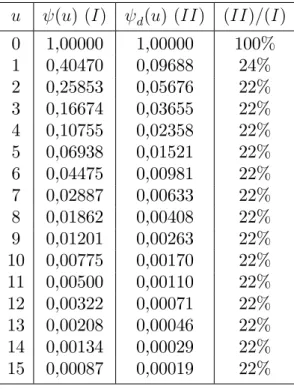
Table 3.1 shows the exact ruin probability and the exact ruin probability caused by oscillation. The third column shows the weight of this form of ruin in the total ruin probability. We can see that it has quite some impact when compared to the mixture of exponentials presented in the next section, that has a heavier tail.
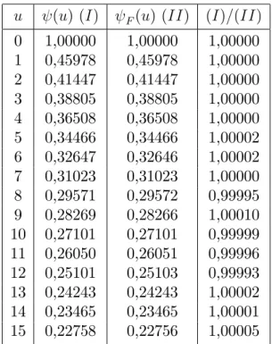
Although we know the exact ruin probabilities we present the numerical results of the methods proposed during this work, to test the behaviour of the approximations in the exponential case. Table 3.2 shows the results for Beekman-Bowers’, Tijms’ and Fourier methods. The De Vylder’s approximation is not presented because in this case it is reduced to the exact ruin probability and the bounds are not needed because we can use the exact probability to test the results. In order to be possible to approximate the ruin probability using the Fourier transform we must split p(x)(s)
u (u) (I) d(u) (II) (II)=(I) 0 1,00000 1,00000 100% 1 0,40470 0,09688 24% 2 0,25853 0,05676 22% 3 0,16674 0,03655 22% 4 0,10755 0,02358 22% 5 0,06938 0,01521 22% 6 0,04475 0,00981 22% 7 0,02887 0,00633 22% 8 0,01862 0,00408 22% 9 0,01201 0,00263 22% 10 0,00775 0,00170 22% 11 0,00500 0,00110 22% 12 0,00322 0,00071 22% 13 0,00208 0,00046 22% 14 0,00134 0,00029 22% 15 0,00087 0,00019 22%
Table 3.1: Exact …gures, Exponential.
into the real and the complex part. In the exponential( ) case we have,
r p(x)(s) = 2 2+s2 c p(x)(s) = s 2+s2
We can see by the ratio between (I) and (II) that the Beekman-Bowers approx-imation is, of the three, the worst. Tijms’approxapprox-imation and the Fourier method revealed to be excellent approximations. This is mainly due to the fact that in this case rp(x)(s) and
c
p(x)(s) are non problematic functions to apply into (2:7) and so
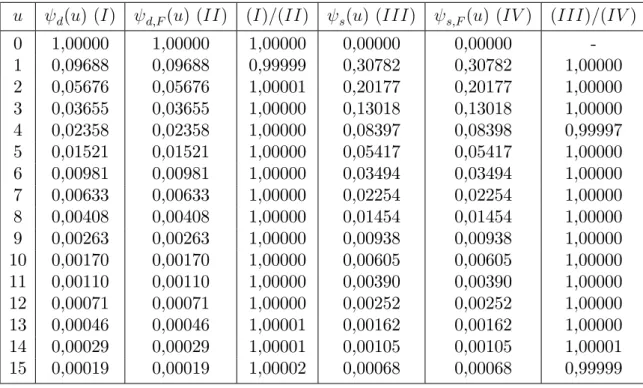
the software calculates the integral nice and easy, without accumulate to many nu-merical errors. Table 3.3 shows the application of the Fourier method for d(u)and
s(u) which also revealed to be an excellent approximation.
3.2
Mixture of exponentials
The claim amount distribution of this example is taken from Wikstad (1971), case IIA. The distribution function of the mixture of exponentials presented there has the following form:
u (u) (I) BB(u) (II) (I)=(II) T(u) (III) (I)=(III) F(u) (IV ) (I)=(IV ) 0 1,00000 1,00000 1,00000 1,00000 1,00000 1,00000 1,00000 1 0,40470 0,39819 1,01633 0,40470 1,00000 0,40470 1,00000 2 0,25853 0,26155 0,98847 0,25853 1,00000 0,25853 1,00000 3 0,16674 0,17096 0,97529 0,16674 1,00000 0,16674 1,00000 4 0,10755 0,11049 0,97345 0,10755 1,00000 0,10755 1,00000 5 0,06938 0,07089 0,97866 0,06938 1,00000 0,06937 1,00000 6 0,04475 0,04526 0,98874 0,04475 1,00000 0,04475 1,00000 7 0,02887 0,02879 1,00253 0,02887 1,00000 0,02887 1,00000 8 0,01862 0,01827 1,01929 0,01862 1,00000 0,01862 1,00000 9 0,01201 0,01156 1,03859 0,01201 1,00000 0,01201 1,00000 10 0,00775 0,00731 1,06010 0,00775 1,00000 0,00775 1,00000 11 0,00500 0,00461 1,08364 0,00500 1,00000 0,00500 1,00000 12 0,00322 0,00291 1,10906 0,00322 1,00000 0,00322 1,00000 13 0,00208 0,00183 1,13627 0,00208 1,00000 0,00208 1,00000 14 0,00134 0,00115 1,16520 0,00134 1,00000 0,00134 1,00000 15 0,00087 0,00072 1,19580 0,00087 1,00000 0,00087 1,00000
Table 3.2: Beekman-Bowers’, Tijms’and Fourier methods, Exponential.
u d(u) (I) d;F(u) (II) (I)=(II) s(u) (III) s;F(u) (IV ) (III)=(IV )
0 1,00000 1,00000 1,00000 0,00000 0,00000 -1 0,09688 0,09688 0,99999 0,30782 0,30782 1,00000 2 0,05676 0,05676 1,00001 0,20177 0,20177 1,00000 3 0,03655 0,03655 1,00000 0,13018 0,13018 1,00000 4 0,02358 0,02358 1,00000 0,08397 0,08398 0,99997 5 0,01521 0,01521 1,00000 0,05417 0,05417 1,00000 6 0,00981 0,00981 1,00000 0,03494 0,03494 1,00000 7 0,00633 0,00633 1,00000 0,02254 0,02254 1,00000 8 0,00408 0,00408 1,00000 0,01454 0,01454 1,00000 9 0,00263 0,00263 1,00000 0,00938 0,00938 1,00000 10 0,00170 0,00170 1,00000 0,00605 0,00605 1,00000 11 0,00110 0,00110 1,00000 0,00390 0,00390 1,00000 12 0,00071 0,00071 1,00000 0,00252 0,00252 1,00000 13 0,00046 0,00046 1,00001 0,00162 0,00162 1,00000 14 0,00029 0,00029 1,00001 0,00105 0,00105 1,00001 15 0,00019 0,00019 1,00002 0,00068 0,00068 0,99999
This distribution is described by Wikstad as an attempt to model the Swedish non-industrial …re insurance data from 1948-1951. It is a highly skewed distri-bution, with variance of 42,1982 and skewness of 27,6873. Here we get H2(x) =
1 0:16106e 5:514588x 0:56696e 0:190206x 0:271977e 0:014631x. The exact …gures for (u)and d(u)can be seen at table 3.4. We can note that in this case the weight of the di¤usion to ruin is much smaller than in the case of the exponential distribution.
u (u) (I) d(u) (II) (II)=(I)
0 1,00000 1,00000 100% 1 0,45978 0,04326 9% 2 0,41447 0,01473 4% 3 0,38805 0,01220 3% 4 0,36508 0,01081 3% 5 0,34466 0,00963 3% 6 0,32647 0,00859 3% 7 0,31023 0,00767 2% 8 0,29571 0,00687 2% 9 0,28269 0,00616 2% 10 0,27101 0,00554 2% 11 0,26050 0,00499 2% 12 0,25101 0,00451 2% 13 0,24243 0,00408 2% 14 0,23465 0,00371 2% 15 0,22758 0,00338 1%
Table 3.4: Exact …gures, Mixture of Exponentials.
The results of the approximation methods can be seen in table 3.5. The …gures do not seem to be impressive in any case. We remember that these three methods are based on the idea of equating a few moments in order to obtain closed formula approximations. As the distribution is highly skewed, the few moments here do not seem to be enough to obtain good results. If we computed the Tijms’approximation for a large enough u we would get good results but it would be essentially due to the asymptotic result. However the inversion of the Fourier transform produced good results as we can see in the tables 3.6 and 3.7. The real and the complex parts of
u (u) (I) DV(u) (II) (I)=(II) BB(u) (III) (I)=(III) T(u) (IV ) (I)=(IV ) 0 1,00000 1,00000 1,00000 1,00000 1,00000 1,00000 1,00000 1 0,45978 0,73340 0,62691 0,42460 1,08284 0,75482 0,60912 2 0,41447 0,55758 0,74334 0,38253 1,08351 0,58596 0,70734 3 0,38805 0,44134 0,87925 0,36101 1,07491 0,46942 0,82666 4 0,36508 0,36420 1,00241 0,34439 1,06008 0,38875 0,93911 5 0,34466 0,31274 1,10209 0,33053 1,04277 0,33270 1,03597 6 0,32647 0,27812 1,17383 0,31852 1,02497 0,29352 1,11226 7 0,31023 0,25458 1,21859 0,30785 1,00771 0,26592 1,16663 8 0,29571 0,23831 1,24085 0,29823 0,99153 0,24626 1,20077 9 0,28269 0,22682 1,24632 0,28944 0,97668 0,23207 1,21816 10 0,27101 0,21848 1,24042 0,28133 0,96331 0,22162 1,22289 11 0,26050 0,21222 1,22750 0,27380 0,95142 0,21374 1,21874 12 0,25101 0,20732 1,21075 0,26675 0,94099 0,20765 1,20885 13 0,24243 0,20333 1,19230 0,26013 0,93195 0,20277 1,19559 14 0,23465 0,19995 1,17357 0,25389 0,92425 0,19875 1,18067 15 0,22758 0,19697 1,15538 0,24797 0,91776 0,19531 1,16520
Table 3.5: De Vylder’s, Beekman-Bowers’and Tijms’methods, Mixture of Exponentials.
p(x)(s) in a mixture of n-exponentials are given by r p(x)(s) = n P i=1 Ai 2i 2 i+s2 c p(x)(s) = n P i=1 sAi i 2 i+s2
The results are not so good as for the case of the exponential distribution due, we believe, essentially two things: 1) rp(x)(s) and cp(x)(s)are harder to compute in (2:7)than before; 2) the values of the 0isand A0
isin this distribution are much more
likely to produce and accumulate numerical errors than just a = 1 and a A = 1. Despite the small di¤erences to the exact values, this method is still an excellent approximation.
3.3
Gamma distribution
We consider now that the claim amount distribution is gamma(2,2), with density function p(x) = 4xe 2x and distribution function P (x) = 1 (1 + 2x)e 2x which
implies H2(x) = 1 (1 + x)e 2x. We do not have exact …gures for this distribution
so in order to test the accuracy of the methods we computed Dufresne & Gerber’s bounds with # = 0:01 to use as a comparison basis. To apply the Fourier method
u (u) (I) F(u) (II) (I)=(II) 0 1,00000 1,00000 1,00000 1 0,45978 0,45978 1,00000 2 0,41447 0,41447 1,00000 3 0,38805 0,38805 1,00000 4 0,36508 0,36508 1,00000 5 0,34466 0,34466 1,00002 6 0,32647 0,32646 1,00002 7 0,31023 0,31023 1,00000 8 0,29571 0,29572 0,99995 9 0,28269 0,28266 1,00010 10 0,27101 0,27101 0,99999 11 0,26050 0,26051 0,99996 12 0,25101 0,25103 0,99993 13 0,24243 0,24243 1,00002 14 0,23465 0,23465 1,00001 15 0,22758 0,22756 1,00005
Table 3.6: Fourier method, Mixture of Exponentials.
u d(u) (I) d;F(u) (II) (I)=(II) s(u) (III) s;F(u) (IV ) (III)=(IV )
0 1,00000 1,00000 1,00000 0,00000 0,00000 -1 0,04326 0,04326 0,99998 0,41651 0,41652 1,00000 2 0,01473 0,01473 1,00004 0,39975 0,39975 0,99999 3 0,01220 0,01220 1,00025 0,37585 0,37585 0,99999 4 0,01081 0,01081 1,00042 0,35427 0,35427 0,99999 5 0,00963 0,00961 1,00181 0,33503 0,33505 0,99997 6 0,00859 0,00857 1,00194 0,31788 0,31789 0,99997 7 0,00767 0,00767 0,99999 0,30256 0,30256 1,00000 8 0,00687 0,00690 0,99542 0,28884 0,28882 1,00006 9 0,00616 0,00609 1,01118 0,27653 0,27657 0,99986 10 0,00554 0,00554 0,99991 0,26547 0,26547 0,99999 11 0,00499 0,00501 0,99571 0,25551 0,25550 1,00004 12 0,00451 0,00454 0,99179 0,24651 0,24649 1,00008 13 0,00408 0,00406 1,00445 0,23835 0,23836 0,99995 14 0,00371 0,00370 1,00213 0,23095 0,23095 0,99998 15 0,00338 0,00334 1,00955 0,22420 0,22422 0,99991
in this case, we used the following decomposition of the gamma( ; ) transform, r p(x)(s) = cos( ) c p(x)(s) = sin( ) with = p 2 +s2 and = arccos( )
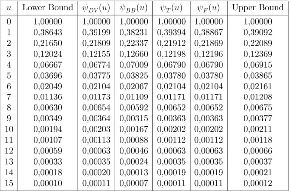
Table 3.8 shows the results of the approximations. We can see that the only really poor approximation is the Beekman-Bowers’, with almost every values outside the bounds. Tijms’and De Vylder’s approximations only miss the bound at u = 1 and the Fourier method reproduce …gures inside the bounds for all values of u.
u Lower Bound DV(u) BB(u) T(u) F(u) Upper Bound
0 1,00000 1,00000 1,00000 1,00000 1,00000 1,00000 1 0,38643 0,39199 0,38231 0,39394 0,38867 0,39092 2 0,21650 0,21809 0,22337 0,21912 0,21869 0,22089 3 0,12024 0,12155 0,12660 0,12198 0,12196 0,12369 4 0,06667 0,06774 0,07009 0,06790 0,06790 0,06915 5 0,03696 0,03775 0,03825 0,03780 0,03780 0,03865 6 0,02049 0,02104 0,02067 0,02104 0,02104 0,02161 7 0,01136 0,01173 0,01109 0,01171 0,01171 0,01208 8 0,00630 0,00654 0,00592 0,00652 0,00652 0,00675 9 0,00349 0,00364 0,00315 0,00363 0,00363 0,00377 10 0,00194 0,00203 0,00167 0,00202 0,00202 0,00211 11 0,00107 0,00113 0,00088 0,00112 0,00112 0,00118 12 0,00059 0,00063 0,00046 0,00063 0,00063 0,00066 13 0,00033 0,00035 0,00024 0,00035 0,00035 0,00037 14 0,00018 0,00020 0,00013 0,00019 0,00019 0,00021 15 0,00010 0,00011 0,00007 0,00011 0,00011 0,00012
Table 3.8: Dufresne & Gerber’s Bounds, De Vylder’s, Beekman-Bowers’, Tijms’and Fourier Methods, Gamma.
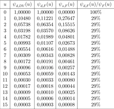
Since that the De Vylder’s approximation revealed to be adjusted to this dis-tribution we decided to present also the approximation to d(u) by this method, along with the Fourier method. Table 3.9 shows the results. Here we do not have a comparison basis but judging from the previous results we believe that d;F(u)
and s;F(u) are the closest to the exact values. Given this, we present also the ratio between d;F and F where we can see that the contribution of oscillations
exponentials presented in the previous section and it has also more weight than in the case of the exponential distribution, which has a heavier tail than the gamma.
u d;DV(u) d;F(u) s;F(u) d;F(u)= F(u) 0 1,00000 1,00000 0,00000 100% 1 0,10480 0,11221 0,27647 29% 2 0,05738 0,06354 0,15515 29% 3 0,03198 0,03570 0,08626 29% 4 0,01782 0,01989 0,04801 29% 5 0,00993 0,01107 0,02673 29% 6 0,00554 0,00616 0,01488 29% 7 0,00309 0,00343 0,00828 29% 8 0,00172 0,00191 0,00461 29% 9 0,00096 0,00106 0,00257 29% 10 0,00053 0,00059 0,00143 29% 11 0,00030 0,00033 0,00080 29% 12 0,00017 0,00018 0,00044 29% 13 0,00009 0,00010 0,00025 29% 14 0,00005 0,00006 0,00014 29% 15 0,00003 0,00003 0,00008 29%
Table 3.9: De Vylder’s and Fourier methods for d(u) and s(u), Gamma.
3.4
Pareto distribution
In this last example we consider that the claim amount distribution follows a Pareto(5,4) with density function p(x) = (4+x)5 456 and distribution function P (x) = 1
4 x+4 5 . This leads to H2(x) = 1 x+44 4
. Tijms’ approximation is not applicable be-cause the moment generating function of the Pareto distribution does not exist. The Fourier method is applicable but as the Pareto distribution does not have an explicit form for the characteristic function we need to calculate numerically the integralsR0+1cos(sx)p(x)dx and R0+1sin(sx)p(x)dx to apply the inversion formula (2:7). Table 3.10 shows the results for De Vylder’s, Beekman-Bowers’and Fourier methods. In this case we also do not have exact …gures for the ruin probability so we calculated Dufresne & Gerber’s bounds, again with # = 0:01.
Both Beekman-Bowers’ and De Vylder’s approximations revealed a poor …t to this distribution with the majority of the values outside the bounds. Although
u Lower Bound DV(u) BB(u) F(u) Upper Bound 0 1,00000 1,00000 1,00000 1,00000 1,00000 1 0,40867 0,45521 0,38282 0,41036 0,41206 2 0,27697 0,24441 0,27165 0,27853 0,28011 3 0,19577 0,15464 0,20096 0,19707 0,19838 4 0,14124 0,11033 0,15017 0,14229 0,14336 5 0,10339 0,08437 0,11286 0,10423 0,10509 6 0,07656 0,06680 0,08516 0,07723 0,07792 7 0,05724 0,05373 0,06443 0,05778 0,05832 8 0,04317 0,04353 0,04886 0,04359 0,04402 9 0,03280 0,03537 0,03712 0,03314 0,03348 10 0,02511 0,02879 0,02824 0,02537 0,02564 11 0,01935 0,02344 0,02151 0,01956 0,01977 12 0,01501 0,01909 0,01640 0,01518 0,01534 13 0,01172 0,01555 0,01251 0,01185 0,01198 14 0,00920 0,01266 0,00956 0,00931 0,00941 15 0,00727 0,01032 0,00730 0,00736 0,00744
Table 3.10: Dufresne & Gerber’s Bounds, De Vylder’s and Beekman-Bowers’ methods,
Pareto.
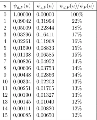
this distribution does not have a very high variance, its skewness of approximately 4.65, which is greater than in the case of the exponential or the gamma presented before, can help to explain the poor …t of these two methods. The Fourier method produced values inside the bound for all u. The approximations to the decomposed probabilities using this method can be seen in table 3.11 along with the ratio between
d;F and F. We can see that the contribution of the di¤usion component to the
occurence of ruin is again less considerable, when compared with the exponential or gamma distributions, which is expectable due to the fact that the Pareto distribution is a well known example of a heavy tail distribution.
u d;F(u) s;F(u) d;F(u)= F(u) 0 1,00000 0,00000 100% 1 0,09042 0,31994 22% 2 0,05009 0,22844 18% 3 0,03296 0,16411 17% 4 0,02261 0,11968 16% 5 0,01590 0,08833 15% 6 0,01138 0,06585 15% 7 0,00826 0,04952 14% 8 0,00606 0,03753 14% 9 0,00448 0,02866 14% 10 0,00334 0,02203 13% 11 0,00251 0,01705 13% 12 0,00190 0,01327 13% 13 0,00145 0,01040 12% 14 0,00111 0,00820 12% 15 0,00085 0,00650 12%
Conclusions
Looking at the …gures of the approximations presented, a …rst conclusion we should underline is the poor …t of the Beekman-Bowers’approximation method, no matter the distribution example. Similar conclusions had been taken by Jacinto (2008), who …rst tried this kind of approximation. The approximations by De Vylder and Tijms look capable of producing good results if the claim amount distribution is well behaved. It is, at least, the case of the exponential or gamma distributions, when opposed to the mixture of exponentials and Pareto distributions. These two methods have the advantage of being very simple to compute and they do not require much software power. In other cases, good approximations can be obtained by computing Dufresne & Gerber’s method of bounds, or using the Fourier transform method. Although these two approaches require a more powerful software, like Mathematica, in order to calculate recursive sums or more complex integrals, they provide much more precise results.
In short, we have adapted from the classical Cramér-Lundberg model to the per-turbed model some simple methods to approximate the ultimate ruin probability. Some of the methods behave simultaneously well in both cases, others behave well in the classical model but not in the perturbed model and others do not work sat-isfactory in either case. Also, the results obtained to the ruin probability caused by di¤usion seem to leave the idea that the di¤usion component can have a substantial part in the ultimate ruin probability, specially if the claim amount distribution is light tailed. Obviously, if we increase the value of the perturbation, , this probab-ility will go up. As the classical model and the illustrations for di¤erent are not dealt in this work, see for instance Jacinto (2008) for some numerical examples.
Concerning the ultimate ruin probability in the classical risk process perturbed by di¤usion we think that we have obtained satisfactory results. Future works can be developed dropping the Poisson assumption an generalize to other renewal risk models with a perturbation by di¤usion.
A
Wiener process and moments of V(t)
De…nition 5 A stochastic process fW (t); t 0g is said to be a Standard Wiener Process if
i) W (0) = 0;
ii) fW (t); t 0g has stationary and independent increments;
iii) for every t > 0, W (t) is normally distributed with mean 0 and variance t
We can generalize the standard Wiener process into a Wiener process with di¤u-sion, i.e. if fW (t)gt 0 is a standard Wiener process, f W (t)gt 0 is a Wiener process
with di¤usion coe¢ cient 2 > 0.
From iii) we can conclude that the density function of W (t) is given by
fW (t)(x) =
1 p
2 te
x2=2t
and from ii) we can conclude that for t0 < t1 < < tn, W (t1) W (t0); ; W (tn)
W (tn 1) are independent and due to stationarity, W (t + s) W (s), is normally
distributed with mean 0 and variance t, for s > 0.
The moments of S(t) = PN (t)t=1 Xi are well known from the actuarial literature,
the deduction of them can be seen for instance at Gerber (1979). The …rst four raw moments are given by,
E[S(t)] = tp1 E[S2(t)] = 2t2p21+ tp2 E[S3(t)] = 3t3p31+ 3 2t2p1p2+ tp3 E[S4(t)] = 4t4p41+ 6 3t3p21p2+ 3 2t2p22+ 4 2 t2p1p3+ tp4
moments of the perturbed surplus process fV (t)g; E[V (t)] = u + ct tp1 V [V (t)] = 2t + tp2 E[(V (t) E[V (t)])3] = tp3 E[(V (t) E[V (t)])4] = tp4 + 3 2t2p22+ 6 t 2 p2 2+ 3 4t2
B
Convolutions
De…nition 6 The convolution operation between two general functions f (:) and g(:) is de…ned by
f g(z) = Z +1
1
f (x)g(z x)dx x2 <
In probability theory, we can use the convolution operator to …nd the distribution of a random variable that is a sum of other two.
Theorem 12 If X and Y are two continuous and independent random variables with probability distribution function FX(x), FY(y) and probability density function
fX(x), fY(y), respectively. Then the probability distribution function of Z = X + Y
is given by FZ(z) = FX FY(z) = Z +1 1 FX(z y)fY(y)dy = Z +1 1 FY(z x)fX(x)dx
the respective density function of Z is given by
fZ(z) = fX fY(z) = Z +1 1 fX(z y)fY(y)dy = Z +1 1 fY(z x)fX(x)dx Proof. FZ(z) = Pr(X+Y z) = RR x+y z fX(x)fY(y)dxdy = R+1 1 Rz y 1 fX(x)fY(y)dxdy = R+1
1 FX(z y)fy(y)dy:Di¤erentiating FZ(z)in order do z we get fZ(z) = d dz R+1 1 FX(z y)fY(y)dy = R+1 1 fX(z y)fY(y)dy.
If X and Y are two positive random variables it is important to note that fX(:)
and fY(:)are concentrated on (0; +1) and therefore the convolution is reduced to
fX fY(z) =
Rz
0 fX(z y)fY(y)dy =
Rz
0 fY(z x)fX(x)dx. The same happens with
FX FY(z).
De…nition 7 The n-fold convolution of FX(x), denoted by FXn(x), represents the
distribution function of the sum of n mutually independent random variables with common distribution FX(x) and it is de…ned iteratively. For n = 0 we have,
FX0(x) = 8 < : 0 if x < 0 1 if x 0
and for 1; 2; ; n we have, FXn(x) = Z +1 1 FX(n 1)(x y)dFX(y) = F (n 1) X FX(x)
If we are only in the presence of non negative random variables, F n
X (x)is reduce to F n X (x) = Rx 0 F (n 1)
C
Laplace transform
We just present here some basic properties but for a deeper insight about this transform see for instance Poularikas (1996).
Let f (x) be a continuous function de…ned for x 0 whose integral exists for all x > 0. Its Laplace transform is de…ned as
f (s) = Z +1
0
e sxf (x)dx
if the integral is convergent. If f (x) is a probability density function of a non negative random variable then the Laplace transform exists at least for s 0. We can also see the Laplace transform as LX(s) = E[e sX] and with this calculate the
raw moments of a random variable: dk
dskLX(s) = E[( X) ke sX]
evaluating at s = 0 we get E[( X)k]. The Laplace transform is analogous to the
Moment Generating function of a random variable, the advantage is that if the random variable is non negative, the Laplace transform exists at least for s 0.
Property 1 Let f (:) and g(:) be functions with Laplace transform and let a and b be constants. Then,
Z +1
0
e sy[af (y) + bg(y)]dy = af (s) + bg(s)
Property 2 Let F (x) =R0xf (y)dy, then
F (s) = 1 sf (s)
Property 3 Let f (y) be a continuous and di¤erentiable function de…ned for x 0. Then,
Z +1 0
e sy d
Property 4 Let ffj(:)gnj=1 be functions which the Laplace transforms exist and let
h(x) be the n-fold convolution of them, i.e. h(x) = f1 f2 fn(x). Then
the Laplace transform of h(x) is
h(s) =
n
Y
j=1
D
Renewal theory
We present here some basic notions of Renewal Theory that are used to obtain the asymptotic results for the ruin probabilities. A deeper insight about this matter can be found for instance at Feller (1971).
De…nition 8 Let H(x) be a proper distribution function concentrated on (0; +1), such that H(0) = 0 and H(1) = 1. Because of the assumed positivity we can safely write = Z 1 0 ydH(y) = Z 1 0 (1 H(y)) dy where 1. When =1 we interpret the symbol 1 as 0.
De…nition 9 A proper renewal equation is de…ned as an equation of the form
Z(x) = z(x) + Z x
0
Z(x y)dH(y); x 0 (D.1)
For x 0, the quantities H(x) and z(x) are known and Z(x) is unknown. One of the major goals of the Renewal Theory is to study the asymptotic behaviour of the solution Z of the equation (D:1). Feller (1971) proved the following renewal theorem that gives a solution to this problem.
Theorem 13 If z(x) is directly Riemann integrable and H(:) is non arithmetic it follows that Z(x)! 1 Z 1 0 z(y)dy as x ! 1.
An important generalization of the renewal process that is very useful in ruin theory is obtained when H(:) is a defective distribution, i.e. H(1) < 1. Such process is called terminating or transient process. The defect 1 H(1) is the probability of extinction.
De…nition 10 A defective renewal equation is de…ned as an equation of the form Z(x) = z(x) + Z x 0 Z(x y)dH(y); x 0 with H(1) < 1.
A very useful and standard argument used in renewal theory, when we have a transient processes is that there exists a number such that,
Z 1 0
e ydH(y) = 1 (D.2)
If the integral exists, the root is unique and as the distribution H(:) is defective, > 0:
De…ning
dH#(y) = e ydH(y)
we have by (D:2) that H#(y) is now a proper probability distribution because
H#(
1) = 1. Also, we associate with any general function f(:), another function f#(:) de…ned as,
f#(x) = e xf (x)
Applying this transformation to each element of a defective renewal equation we obtain the following equation, that is now a proper renewal equation (please see Feller (1971) for further details),
Z#(x) = z#(x) + Z x
0
Z#(x y)dH#(y), x 0
and if z#(x)is directly Riemann integrable, the Renewal Theorem implies, for a non
arithmetic H#(:)that, e xZ(x)! 1 # Z 1 0 e yz(y)dy where # = Z 1 0 ye ydH(y)
E
Proofs
We present here the proof of d(0) = 1, the expression for ML(s)(expression (1:17))
and the deduction of the asymptotic result for d(u) (expression (1:18)).
Proof of d(0) = (0) = 1 . De…ning d = infft 0 : W (t) + ct < 0g we have
that,
f d tg fW (t) + ct < 0g ) Prf d tg PrfW (t) + ct < 0g = ( ct)
As (:) is the distribution function of a Normal(0,1), ( ct) is always positive. Taking the limit we have:
Prf d= 0g = lim
t!0+Prf d tg ( ct):
by the Blumenthal’s law (see for instance Mörters and Peres (2010)) we have that Prf d = 0g = 1, i.e, the Weiner process with drift can almost surely take negative
values immediately after its beginning.
Given this and given that N (0) = 0, we have d(0) = (0) = 1.
Proof of ML(s). If we consider Li = L (1) i + L (2) i f or i = 1; : : : ; M we can write ML(s) as: ML(s) = E[esL (1) 0 +s PM i=0Li] = E[esL (1) 0 ]E[es PM i=0Li] = M L(1)0 (s)MM[ln(ML (s))] (E.1) where MM(s) = q 1 (1 q)es = c p1 c es p 1 (E.2) ML(1) 0 = s (E.3)
B to see the properties of convolutions, we obtain, ML (s) = Z 1 0 esxh1 h2(x)dx = Z 1 0 Z x 0 esxh1(y)h2(x y)dydx = Z 1 y=0 h1(y) Z 1 x=y esx[1 P (x y)] p1 dxdy = p11 Z 1 0 h1(y) Z 1 y Z 1 x y esxp(v)dvdxdy = = p11 Z 1 0 h1(y) Z 1 v=0 p(v) Z v+y y esxdxdvdy = (sp1) 1 Z 1 0 h1(y) Z 1 0 p(v)esv+sydv Z 1 0 p(v)esydv dy = (sp1) 1 Z 1 0 h1(y) [esyMX(s) esy] dy = = (sp1) 1 Z 1 0 h1(y)esy [MX(s) 1] dy = (sp1) 1[MX(s) 1] ML(1) 0 (s) (E.4)
so if we apply (E:2), (E:3) and (E:4) into (E:1), we obtain (1:17) :
Proof of d(u). We present the deduction for (1:18) but (1:19) and (1:20) can be obtain in a similar way starting from (1:3) and (1:4), respectively. The starting point here is the defective renewal equation (1:2). According to the notation presented in Appendix D we have,
Z(u) = d(u); z(u) = 1 H(u); H(x) = (1 q)R0xh1 h2(y)dy
Equation (1:2) is defective because H(1) = (1 q) < 1. So, supposing that exists a number such that R01e xdH(x) = 1, we have
(1 q) Z 1
0
= (1 q) Z 1 0 e x Z x 0 h1(y)h2(x y)dydx = (1 q) Z 1 0 h1(y) Z 1 y e x1 P (x y) p1 dxdy = c Z 1 0 h1(y) Z 1 y e x Z 1 x y p(v)dvdxdy = c Z 1 0 h1(y) Z 1 0 p(v) Z v+y y e xdxdvdy = c Z 1 0 h1(y) Z 1 0 p(v)e (v+y) e y dvdy = c Z 1 0 h1(y)e y Z 1 0 p(v) [e v 1] dvdy = c Z 1 0 e y e y Z 1 0 p(v)e vdv Z 1 0 p(v)dv dy = c Z 1 0 p(v)e vdv 1 = 2 2c 2 2 Z 1 0 p(v)e vdv 1
And by the de…nition of the adjustment coe¢ cient, equation (1:5), we can note that the only possible solution for R01e xdH(x) = 1, is when = R. Applying eRx to
each function of equation (1:2), we arrive to
eRu d(u) = eRu[1 H1(u)] + (1 q)
Z u 0
eR(u x) d(u x)eRxh1 h2(x)dx
Which is now a proper renewal equation for the function eRu
d(u)and according to
the renewal theorem we have that
eRu d(u)! R1 0 e Rx[1 H 1(x)] dx (1 q)R01xeRxh 1 h2(x)dx = Cd
which is the same as
References
Beekman, J., (1969). A ruin function approximation, Trans. Soc. Actuaries, 21, 41–48 and 275–279.
De Vylder, F. (1978). A practical solution to the problem of ultimate ruin probab-ility. Scandinavian Actuarial Journal , 1978 (2):114–119.
Dickson, D.C.M. (2005). Insurance risk and ruin, Cambridge: Cambridge University Press.
Dufresne, F. and Gerber, H.U. (1989).Three methods to calculate the probability of ruin, ASTIN Bulletin, 19 (1):71-90.
Dufresne, F. and Gerber, H.U. (1991). Risk theory for the compound Poisson process that is perturbed by di¤usion, Insurance: Mathematics and Economics, 10:51-59. Feller, W. (1971). An introduction to Probability Theory and its Applications, Vol
II, 2nd Ed. New York: John Wiley & Sons.
Gerber, H.U. (1979). An introduction to Mathematical Risk Theory, S.S. Huebner Foundation for Insurance Education, University of Pennsylvania, Philadelphia, Pa. 19104, USA.
Jacinto, A.C.F.S. (2008). Aproximações à probabilidade de ruína no modelo perturb-ado, Master thesis, ISEG Technical University of Lisbon.
Kaas, R., Goovaerts, M., Dhaene, J. and Denuit, M. (2008). Modern Actuarial Risk Theory: Using R, 2nd edition, Springer.
Klugman, S., Panjer, H. and Willmot, G. (2008). Loss models: from data to de-cisions, 3rd edition.Hoboken, N.J.: John Wiley & Sons.
Lima, F.D.P., Garcia, J.M.A and Egídio dos Reis, A.D. (2002). Fourier/Laplace transforms and ruin probabilities, ASTIN Bulletin 32(1), 91-105.
Mörters, P. and Peres, Y. (2010). Brownian Motion, Cambridge: Cambridge Uni-versity Press.
Panjer, H.H. (1981). Recursive evaluation of a family of compound distributions, ASTIN Bulletin, 12(1):22–26.
Poularikas, A. (1996).The transforms and applications handbook, Boca Raton: CRC Press.
Silva, M.D.V. (2006). Um Processo de Risco Perturbado: Aproximações Numéricas à Probabilidade de Ruína, Master Thesis, Faculty of Science University of Oporto.
Tijms, H. (1994). Stochastic Models - An Algorithmic Approach, Chichester: John Wiley & Sons.
Wikstad, N. (1971). Exempli…cation of ruin probabilities, ASTIN Bulletin, 6(2):147– 152.