Mestrado em Medicina Veterinária
Dissertação
Évora, 2019
Prognostic Value of Volume-Weighted Mean Nuclear
Volume in Canine Mast Cell Tumours
Mafalda Casanova da Costa Martins
Orientação interna: Professora Doutora Sandra Branco
Orientação externa: Professor Doutor Pedro Faísca
Professora Doutora Leonor Orge
ESCOLA DE CIÊNCIAS E TECNOLOGIA
I
O júri de provas foi constituído por:
Presidente: Rita Payan Carreira
Professora Catedrática – Universidade de Évora
Arguente: Maria dos Anjos Pires
Professora Associada com Agregação – Universidade de Trás-os-Montes e Alto Douro
Orientador: Sandra Maria da Silva Branco Professora Auxiliar – Universidade de Évora
II
Abstract
Cutaneous Mast Cell Tumour (cMCT)’s Patnaik and Kiupel grading schemes rely on qualitative and semi-quantitative features susceptible to bias and inter-observer variability. The stereological estimation of volume-weighted mean nuclear volume (VV),
on the other hand, provides information about both nuclear size and its variability, proven to have prognostic value in many solid tumours.
VV of 55 cMCTs was estimated using the point-sampled intercept method in 10
microscopic fields (800 X). These tumours were graded by three pathologists and the final grade was compared with VV and clinical history of dogs with a follow-up period of one
year.
A cut-off value of VV>168 µm³ was shown to differentiate aggressive cMCTs with
78.3% specificity and 87.5% sensitivity.
The present study suggests that the estimation of VV on routine histological sections may
objectively improve the detection of more aggressive cMCTs.
III
Resumo
Valor Prognóstico do Volume Nuclear Médio em Mastocitomas Caninos
A gradação de Mastocitomas Cutâneos Caninos (cMCTs) pelo sistema de Patnaik e Kiupel é baseado em critérios qualitativos e semi-quantitativos, que estão sujeitos a viés e variabilidade inter-observador. O recurso ao princípio estereológico do ‘volume médio nuclear’ (VV), por outro lado, fornece simultaneamente informação sobre o tamanho
nuclear e a sua variação, o que está associado a um valor de prognóstico em diversos tumores.
O VV de 55 cMCTs foi estimado através do método ‘point-sampled intercept’ em 10
campos microscópicos (800 X). Estes tumores foram classificados por três patologistas e a classificação final foi comparada com o VV e o follow-up clínico de um ano.
Um cut-off de VV>168 µm³ revelou diferenciar cMCTs de comportamento mais
aggressivo com uma especificidade de 78.3% e uma sensibilidade de 87.5%.
Este estudo sugere que o VV poderá objectivamente auxiliar a detecção de cMCTs com
um comportamento mais agressivo.
IV
Index of Contents
Abstract ... II Resumo ... III List of charts ... VI List of tables ... VII List of figures ... VIII List of abbreviations and symbols ... IX Internship report ... II 1. IGC ... II 2. INIAV ... III
I. Literature Review ... 1
1. Introduction ... 1
1.1. Application of stereology in tumour studies ... 2
1.1.1. Particle size... 3
1.2. Estimation of volume-weighted mean nuclear volume (VV) ... 4
1.2.1. PSI method on VUR sections ... 5
1.2.1.1. Orientation frame ... 6
1.2.1.2. Lines associated with points ... 7
1.2.1.3. Counting frame ... 7
1.2.1.4. Logarithmic ruler ... 8
1.2.2. Meaning of VV ... 9
1.2.3. Reproducibility of VV ... 9
2. Canine Mast Cell Tumours ... 11
2.1. Mast cell biology ... 11
2.2. Cutaneous Mast Cell Tumours ... 11
2.3. Prognostic factors ... 12
2.3.1. Tumour Grade ... 13
2.3.1.1. Patnaik grading ... 13
2.3.1.2. Kiupel grading ... 14
2.3.2. Cellular Proliferation ... 15
2.3.3. KIT expression and c-kit mutations ... 16
V
2.3.5. Staging ... 17
II. Research Project ... 19
3. Aim ... 19
4. Materials & Methods ... 20
4.1. Case selection and histopathological analysis ... 20
4.2. Outcomes ... 20 4.3. Stereological estimations ... 20 4.3.1. Field selection... 21 4.3.2. Measurements ... 21 4.3.3. Calculations ... 24 4.4. Statistical analysis ... 26 5. Results ... 27 5.1. Histological grading ... 27 5.2. VV ... 29
5.2.1. Wilcoxon rank-sum test... 29
5.2.2. ROC curve ... 30 5.3. Outcomes ... 31 6. Discussion ... 35 7. Conclusion ... 38 8. References ... 39 9. Appendix section ... i
VI
List of charts
Chart 1a. VV (MNV) vs Patnaik Wilcoxon’s rank-sum test ... 30
Chart 1b. VV (MNV) vs Kiupel Wilcoxon’s rank-sum test ... 30
Chart 2a. VV (MNV) vs Patnaik ROC curve. ... 31
Chart 2b. VV (MNV) vs Kiupel ROC curve ... 31
Chart 3. VV vs Outcome Wilcoxon’s rank-sum test ... 33
Chart 4. VV vs Outcome ROC curve ... 33
VII
List of tables
Table 1. Patnaik and Kiupel grading (adapted from Meuten, 2017). ... 15
Table 2. Nodal metastasis classification ... 18
Table 3. Orientation numbers ... 22
Table 4. Example of general formulas applied in mean nuclear volume (VV) estimations (adapted from Sorensen 1991b, Skau et al. 2001). ... 25
Table 5. Patnaik grading distribution ... 27
Table 6. Patnaik agreement rates ... 28
Table 7. Kiupel grading distribution ... 28
Table 8. Kiupel agreement rates ... 28
Table 9. Patnaik VV values descriptive statistics ... 29
Table 10. Kiupel VV values descriptive statistics ... 29
Table 11. Outcome and tumour grade assignment ... 31
Table 12. Outcome VV values descriptive statistics ... 32
VIII
List of figures
Figure 1. Production of 2D sections across objects (adapted from West, 2012). ... 1
Figure 2. Number and volume-weighted distribution (adapted from Howard & Reed, 2018). ... 3
Figure 3. Point-sampled intercept (adapted from Skau et al. 2001)... 4
Figure 4. Production of an orientation frame (adapted from Sorensen, 1991b). .... 6
Figure 5. Orientation frame (adapted from Sorensen, 1991b). ... 7
Figure 6. Test-lines and equally spaced points ... 7
Figure 7. Counting frame (adapted from Sorensen, 1991b)... 8
Figure 8. Logarithmic ruler (Fehrenbach et al. 2005 - 21). ... 8
Figure 9. Selection of fields. Cutaneous mast cell tumour (cMCT), H&E, Bar 5 mm in overview, bars 50 µm in inserts. ... 21
Figure 10. Orientation frame. cMCT, H&E, Bar 50 µm ... 22
Figure 11. Orientation frame + Test-lines. cMCT, H&E, Bar, 50 µm ... 22
Figure 12. Nuclei point-sampling. cMCT, H&E, Bar, 50 µm ... 23
Figure 13. Intercept length measurement. cMCT, H&E, Bar, 50 µm ... 24
IX
List of abbreviations and symbols
α – Significance LevelAgNOR - Nucleolar Organizer Regions AUC – Area Under the Curve
CI – Confidence Interval
cMCT – Cutaneous Mast Cell Tumour CV – Coefficient of Variation G1 – Grade-I G2 – Grade-II G3 – Grade-III HG – High-grade HN – Histological Node Hpf – High power field HU – Histopathology Unit H&E – Haematoxylin and Eosin IGC – Instituto Gulbenkian de Ciência IHC - Immunohistochemistry
INIAV – Instituto Nacional de
Investigação Agrária e Veterinária
IUR – Isotropic Uniform Random κ – Kappa
KIT - Tyrosine Kinase Receptor LG – Low-grade
𝐥𝟎𝟑 – Cubed intercept length
𝐥̅ – Cubed mean intercept length 𝟎𝟑 𝐋𝐧 – Logarithmic ruler length
M – Magnification MC – Mast Cell
MCT – Mast Cell Tumour VV – Mean Nuclear Volume
IUR – Isotropic Uniform Random OC0 – Outcome of zero
OC1 – Outcome of one P – P-value
PCNA - Proliferating Cell Nuclear
Antigen
PSI – Point Sampled-Intercept ROC – Receivers Operating
Characteristics
SD – Standard Deviation
TSE – Transmissible Spongiform
Encephalopathy
VF – Volume Fraction
VUR – Vertical Uniform Random µm – Micron
II
Internship report
As part of the Integrated Master’s in Veterinary Medicine of Évora University, my internship place at Instituto Gulbenkian de Ciência (IGC) from September 2018 to March 2019, and from November 2018 to February 2019, it was divided between IGC and Instituto Nacional de Investigação Agrária e Veterinária (INIAV). The following dissertation is based on the research developed at IGC.
1. IGC
The IGC is part of Fundação Calouste Gulbenkian, a private charitable foundation promoting innovation in charity, arts, education and science. The IGC is located at the Oeiras campus in Rua da Marinha Grande, home to research programmes of several domains, such as cell and developmental biology, evolutionary biology, plant biology and biophysics. The internship took place at the Histopathology Unit (HU) from September 12th to March 29th, under the orientation of Dr Pedro Faísca. The HU’s mains goals are to provide preparations for microscopic analysis and pathology support to IGC users and associate laboratories, academic institutions and private companies. These services include processing and paraffin embedding, microtome, vibratome and cryotome sectioning, routine and special staining, immunohistochemistry (IHC), pathology assessment and high-quality image acquisition.
The main species observed was the mouse (Mus musculus) and occasionally the zebrafish (Danio rerio). Sporadically, I was also able to observe cell cultures of human hepatocytes and oesophagus. The mouse slides observed included the integumentary system (skin), the respiratory system (lungs, trachea, bronchi, bronchioles), the digestive system and annex organs (stomach, large and small intestine, pancreas, liver and salivary glands), the lymphatic system (spleen, thymus and lymph nodes), the central nervous system (brain and spinal medulla), the urinary system (kidneys), the muscle-skeletal system (skeletal muscle, femur, tibia), the circulatory system (heart), the adipose tissue and the sensory organs (eye). The zebrafish slides included a section of the whole fish. Samples were mainly paraffin-embedded and routinely haematoxylin and eosin (H&E) stained. Occasionally, the pathology assessment required special stains, such as Periodic Acid-Schiff, Masson’s Trichrome and Oil Red.
III
The work of an experimental pathologist was accompanied, which mainly consists in the morphological description of lesions and further comparison of animals from different experimental groups. The main task was the quantification of structures using ImageJ software and Stereology. The slides were digitalized using HAMAMATSU NanoZoomer-SQ Digital slide scanner C13140-01 and opened with NDPI view software. ImageJ quantification included white adipocyte area, lipid area in brown adipocyte tissue and lipid area in Oil Red-stained culture cells. The quantifications were executed manually or semi-automated. Stereological quantifications were mainly focused on Volume, as well as Mean Particle Volume, Number and Surface Area. Stereological estimations were done manually by superposing probes on the screen or using STEPanizer software. Volume estimations often included Volume Fraction (VF) estimations, for example, liver and metastasis VF, skin and epidermis VF, pancreas and pancreatic islets VF or heart and fibrosis VF. Mean particle volume estimations were performed on Barret’s Oesophagus culture cells, canine mast cell tumours and brown adipocyte mitochondria. Number estimations included hair follicle number on dorsal skin and pancreatic islets number.
2. INIAV
INIAV is the public Laboratory of Animal Health, Plant Health, Food and Feed Security. Its reference national laboratories are responsible for the official analysis of numerous zoonoses and antimicrobial resistance. INIAV participates in the surveillance activities of Transmissible Spongiform Encephalopathies (TSEs), a group of diseases caused by the accumulation of abnormal prionic protein in the brain leading to fatal neurodegeneration, such as Bovine Spongiform Encephalopathy, small ruminant Classical and Atypical Scrapie and cervid Chronic Wasting Disease. Such activities include active and passive surveillance of bovine species, sheep, goats and cervids as well as sheep genotyping. This internship took place at the Pathology Laboratory, from November 5th, 2018, to February 28th, 2019, under the supervision of Dr Leonor Orge. Atypical Scrapie was diagnosed in portuguese sheep for the first time in 2004. Following the confirmation, caudal medulla isolates from ARR/ARR and ARQ/ARQ genotypes were sent to the Friedrich-Loeffler-Institut (German National Reference Laboratory for
IV
TSEs) to strain type the form of disease by mouse bioassay. Each isolate was inoculated intracranially in 15 TgshpXI mice expressing ovine PrPARQ, resulting in a total of 30
animals. Incubation periods were monitored, and animals were gradually euthanized after manifesting neurological clinical signs. The brains were formalin-fixed and paraffin-embedded and posteriorly sent to INIAV.
At INIAV, the brains were sectioned at the levels of the medulla, superior colliculus, thalamus and basal ganglia. 5 µm-thick sections were H&E-stained according to standard protocols for histopathology. Lesion profiling was analyzed by the vacuolation severity of nine grey matter areas and three white matter areas. Vacuolation was semi-quantified using a score of 0 to 5 in grey matter areas and 0 to 3 in white matter areas (1).
PrPScdeposition was evaluated by IHC on serial sections of the same coronal areas, according to standard protocols adjusted to mouse brain upon previous testing.
Lesional profiles showed more vacuolation in the hippocampus (G6), cerebral cortex, cerebellar white matter (W1) and cerebral peduncles (W3) in both genotypes. The originally diagnosed sheep had white matter PrPsc deposition at the level of the obex, suggesting a “white matter-type immunolabelling”. A mouse bioassay using tg338 expressing ovine PrPVRQ with isolates from sheep without white matter vacuolation is taking place, to evaluate if these differences are due to a different strain or to a yet unknown cause. The lesional profiles, incubation periods and PrPsc depostion suggest that, independently of sheep genotype, these isolates are concordant with Atypical Scrapie Nor98 transmitted to transgenic tg338 mice. Regarding the possibility of phenotype shifting, it is relevant to pursue strain typing studies.
1
In biology, the observation of three-dimensional objects is enabled by the production of two-dimensional sections. The production of such sections has consequential loss of relation between structures and the number of sections required to section an entire object becomes unpredictable. Solids are observed as profiles, surfaces are observed as lines and lengths are observed as points (Figure 1) (2). Routine histopathology analyses a small fraction of the total organ, and while such amounts may be useful for a qualitative appreciation of the organ’s condition, the same sample will only be suitable for a quantitative analysis if a statistically sound sampling method is applied (3).
Figure 1. Production of 2D sections across objects (adapted from West, 2012).
Stereology is the gold standard method in quantitative studies and allows the recovery of 3D information through estimations, that is, approximations with defined margins of error. Stereological estimates rely on sampling procedures which have various levels that fall into a defined hierarchy: the number of animals, the number of blocks, the number of sections, the number of measurements performed, and the precision of the each individual measurement (2).
Stereological measurements use probes, i.e., geometric shapes (points, lines, cycloids, counting frames) superposed on tissue sections to gather information about the object (2). These probes are applied in a ‘design-based’ scheme, where all structures have the same probability of being sampled, eliminating assumptions about size, shape, orientation or
2
distribution (4). While it is not necessary to sample the whole object, access to the entire object is necessary to ensure that all structures have the same probability of being sampled. Most stereological probes require ‘isotropic’ sampling, where structures are randomly sampled without a preferential orientation (2,5,6).
The efficiency of a procedure is related to the amount of sampling performed, and the margins of error of stereological estimations are defined with statistical principles (accurate sampling, isotropy and randomization). The main goal is to “do more less well!”, in other words, to gather the maximum amount of information at the least effort or cost (2,4,7,8).
The greatest source of variability in stereological estimates comes from the highest sampling levels, especially the biological variances between individuals. The lowest levels, such as the precision of each measurement or feature-to-feature variances have little effect on variability (8).
1.1. Application of stereology in tumour studies
It is well established that tumour cells revealing significant variation in size and larger nuclei will generally be considered aggressive (5,9). Malignant cells have higher mitotic activity and higher nuclei-cytoplasmic ratio than the cells that originate them, accompanied by greater amounts of DNA and clumping of chromatin. These cause the increase of nuclear size and density as well as alterations of chromatin texture. Abnormal metabolic activity also leads to lack of cytoplasmic differentiation and alterations in nucleoli size and shape (6).
Tumour histologic grading relies on the qualitative appreciation of morphological features and has a crucial impact on prognosis and treatment. The subjectivity of tumour grading is not only sensitive to personal bias and knowledge, but also prone to inter-observer variability. An objective and quantitative approach to malignancy severity, on the other hand, provides a significant advantage in terms of reproducibility (6).
Nuclear size quantification can be performed by morphometry, image analysis and stereology. Both morphometry and image analysis rely on area estimations of nuclear profiles, one of the most elusive structures to quantify. A stereological approach, on the
3
other hand, obtains three-dimensional information using a ‘design-based’ scheme, where no assumptions about shape or orientation are made (4,6,10).
1.1.1. Particle size
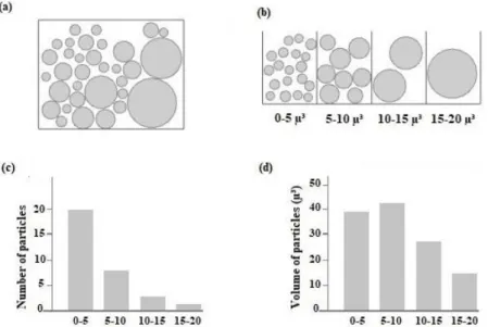
The measurement method applied in particle sizing is based on a measurable criterion, in which every particle is given a ‘weight’. Particles may be sampled according to their height, number, surface area or volume. For examples, if particles are sampled according to their volume, a larger particle will have a greater probability of being sampled (3). Volume estimation can either be number-weighted or volume-weighted, in which particles are sampled according to their number or volume, respectively. Figure 2 illustrates a population of particles of different volumes (a). Each particle is placed in a box with limited spacing. The first box has particles of volume smaller than 5 μ3, the second box has particles greater than 5 μ3 and smaller than 10 μ3, and so on (b). The first histogram reports the number of particles in each bin and is a measure of number-weighted distribution of volume (NV) (c). The second histogram represents the volume
inside each box and provides a measure of volume-weighted distribution of volume (VV)
(d). The same population of particles provides two different aspects of volume distribution (3).
Figure 2. Number and volume-weighted distribution (adapted from Howard & Reed,
4
Volume-weighted estimations of volume are interesting in tumour studies because the mean particle volume mainly reflects the volume of the greater particles. In a number-weighted volume, on the other hand, the mean volume is mainly influenced by the smaller particles.
1.2. Estimation of volume-weighted mean nuclear volume (VV)
The ‘point-sampled intercept method’ was developed by Gundersen and Jensen (1983) and provides a measure of volume-weighted mean nuclear volume (VV) highly suited for
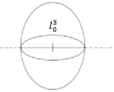
tumour malignancy studies (11). The PSI method samples nuclei using points (+) has an with associated isotropic lines that create an intercept across the nuclear profile (Figure 3). The length of each intercept is measured from nuclear boundary to nuclear boundary (𝑙03) and the mean intercept length provides an unbiased estimation of volume-weighted distribution of volume (3).
Figure 3. Point-sampled intercept (adapted from Skau et al. 2001).
Only a fraction of nuclei is sampled, therefore one measures the volume-weighted mean nuclear volume, which provides information about how large a fraction of the total volume is. One of the advantages of VV application in tumour malignancy is that it
favours nuclear size and therefore contains more information about larger nuclei. It should thus be applied in a situation where larger particles contain valuable information, as is the case in tumour cells (5,6,11,12).
The PSI method requires the assurance of two conditions. Firstly, the observer must be able to distinguish all profiles belonging to the same nucleus (11–13), which, in the case
5
of mononucleated cells can be observed as one single connected profile (11). The second required condition is the assurance of isotropy. Either 1) the structures of interest (particles) are assumed as randomly orientated and a set of arbitrary lines is applied or 2) isotropy is achieved using randomly orientated probes (11). There are three different possibilities:
a) If a structure has a preferred orientation (anisotropic), it is possible to perform Isotropic Uniform Random (IUR) sectioning and application of lines in a fixed direction (5);
b) If a structure is isotropically orientated, a fixed direction can be applied however, assumptions about random orientation should be done carefully;
c) If a nuclear population has a preferred orientation, as is the case in a cutaneous specimen, the PSI method is applied on vertical sections. In this case, nuclear anisotropy is counterbalanced using isotropic sine-weighted orientated lines (9,13).
IUR sections have fixed distance apart and are performed without a preferential orientation. These sampling method often destroys crucial diagnostic information (6). Vertical Uniform Random (VUR) sections, on the other hand, preserve the location of the tumour and are generated by 1) placing an object with a pre-defined horizontal plane on a table and 2) sectioning it perpendicularly to the table. Such horizontal plane is either defined by the observer or corresponds to a region within the tissue (14). In a cutaneous tumour biopsy, the horizontal plane can be defined by the epidermis (14–16).
1.2.1. PSI method on VUR sections
The PSI method requires a set of different probes: 1) an orientation frame which defines the direction of the test-lines; 2) a set of test-lines with equally spaced points that sample nuclei and create intercepts across the nuclear profiles; 3) an orientation frame that samples the area of the field of view for measurement 4) a logarithmic ruler used to measure the length of the nuclear intercepts.
6
1.2.1.1. Orientation frame
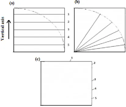
Figure 4 exemplifies the production of an orientation frame. Initially, an arc is projected on the frame along with traced horizontal lines. The lines are traced equidistantly along the vertical axis represented by the left-hand corner of the frame (a). The points where the lines intercept the arc are projected to the centre of the arc (b). The endpoints of the lines generate orientation numbers (c) (15). The orientation frame follows a sine-weighted distribution i.e., the greater the number, the larger the angle to the vertical axis and smaller the distance between numbers (5,15).
Figure 4. Production of an orientation frame (adapted from Sorensen, 1991b).
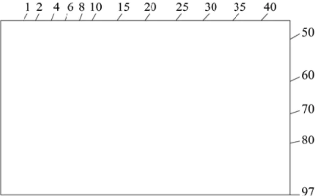
Figure 5 demonstrates the orientation frame composed of 97 numbers used on VV
measurements. Each tumour is generally measured in five to ten fields of view and the initial orientation is randomly generated number between 1 and 97. The test-lines are assembled so one of the lines passes through the generated number and the lower left-hand corner of the frame (17). The following fields have orientations defined by the addition of a constant period of 37 or the subtraction of 60, if the subsequent number is greater than 61 (5,15).
7
Figure 5. Orientation frame (adapted from Sorensen, 1991b).
1.2.1.2. Lines associated with points
A set of equally spaced points (+) samples nuclei and the associated lines select nuclear intercepts for measurement (Figure 6). Whenever a nucleus is hit by two points, it is measured twice (15).
Figure 6. Test-lines and equally spaced points
1.2.1.3. Counting frame
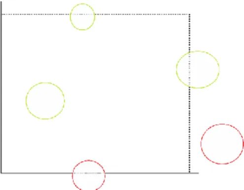
A counting frame composed of inclusion (dashed) and exclusion (full) lines selects the area of the cross-section for measurement. Figure 7 illustrates that nuclei fully or partially within the frame, are sampled (green). Nuclei intercepting the exclusion lines or landing outside the frame are excluded from measurement (red) (5,18).
8
Figure 7. Counting frame (adapted from Sorensen, 1991b).
1.2.1.4. Logarithmic ruler
Although any ruler may be used for intercept measurement, the logarithmic (𝑙03) ruler has the advantage of providing cubed intercept lengths (5). This rule is composed of 15 classes, each 17% wider than the preceding class (Figure 8) (15,19). The ruler length of the magnification must be adjusted so the higher classes correspond to the longest intercepts. If smaller than the latter, a ruler is unsuitable for measurement (10,12).
Figure 8. Logarithmic ruler (Fehrenbach et al. 2005 - 21).
The intercept intercept length (𝑙03) is measured form nuclear boundary to nuclear boundary and falls into one of the classes of the logarithmic ruler. The mean cubed intercept length (𝑙̅ ) is multiplied by 03 𝝅
𝟑 and the mean nuclear volume is obtained.
9
1.2.2. Meaning of VV
If VV and NV are simultaneously estimated from the same population, the coefficient of
variation (CV) of nuclear size can also be measured in a population of tumour cells. CV has also been shown to have prognostic significance and is calculated using Equation 1 (3,15). Despite the interest in knowledge of CV, VV is frequently enough to investigate
tumour malignancy and the description of the distribution of size may be irrelevant.
Equation 1. VV = NV × (1 + CV2)
Equation 1 demonstrates that VV contains information about both size and variability in
size. Therefore, if two specimens present with different VV values, it is not possible to
conclude if these are due to differences in size or due to presence of nuclear pleomorphism (3,15).
1.2.3. Reproducibility of VV
The greatest impact on VV variability seems to be related to biological variation among
patients, with up to 80% total observed variance (9,10). Since the biological variability is always present, the number of fields and intercepts measured have a greater impact on efficiency than variances between fields or the precision of each intercept. The general formula is approximately 75 intercepts per tumour measured in 5 to 10 high power fields (5,6,15). The number of points, lines, and fields also affects efficiency and must be constant for different specimens of the same tumour. Using several points with few lines may lead to the measurement of the same nucleus the same way twice. The absolute magnification and the number of points must be adjusted so that the number of nuclei sampled by two points is decreased to a minimum (6,12).
The unbiased nature of the estimation also relies on tissue processing. Accurate VV
estimations depend on the correct identification and preservation of nuclear profiles. Varying severity areas may present internal variation to tissue processing, and the loss of nuclear profiles on the cross-section has an unpredictable influence on efficiency.
10
One practical solution to this problem is the standardization fixation, dehydration, embedding and sectioning (6).
Since its development, VV has been correlated with histological grading and mortality
rates of various tumours. These include: malignant melanoma (10,21,22), prostatic cancer (23,24), breast cancer (25,26) bladder tumours (27,28) squamous cell carcinoma of the uterine cervix (9) or neuroblastoma (29).
11
2.
Canine Mast Cell Tumours
2.1. Mast cell biology
Mast Cells (MCs) have round central nuclei and variable cytoplasmic granules, involved in inflammatory and immune response. MCs contain high-affinity IgE receptors that trigger the inflammatory mediators upon activation by IgE, a process known as degranulation. These mediators include heparin, histamine, leukotrienes, prostaglandins, proteases, cytokines, chemokines and growth factors (30–32). MC granules are observed with metachromatic stains, such as toluidine blue or the Wright’s combinations, and is caused by binding of mediators to cationic dyes (31,33,34).
MCs are derived from hematopoietic cells originated in the bone marrow, most likely the myelomonocytic line (35). Unlike other hematopoietic cells, pluripotent CD34+ and CD117 leave the bone marrow and enter the bloodstream as undifferentiated precursors of MCs. Differentiation into mature MCs occurs after infiltration of either connective tissue or mucosa. Mature MCs retain the ability to proliferate (36–38).
MCs are ubiquitous in connective tissues, therefore MCTs can develop anywhere in the body (35). In dogs, MCs exist in higher numbers in the skin, lungs, gastrointestinal tract and liver (33,37). The preferential location of MCs is the dermis, near hair follicles and blood vessels. Occasionally MCs can be found in subcutaneous fat (38,39).
2.2. Cutaneous Mast Cell Tumours
Canine mast cell disease usually occurs as single or multiple cutaneous Mast Cell Tumours (MCTs), and less frequently cutaneous or systemic mastocytosis. MCTs arise from the malignant transformation of mast cells and they should always be considered malignant (40,41). Cutaneous MCTs (cMCTs) are the most frequent form of mast cell disease in dogs, followed by subcutaneous MCTs. Extracutaneous MCTs are found in visceral organs such as the liver, spleen, gastrointestinal tract or lung, and are frequently caused by distant metastasis from a cutaneous nodule. Mast cell leukaemia is very rare in dogs (37,38).
cMCTs are one of the most frequently diagnosed skin tumours in dogs (42–44). Although they may be present in dogs of all ages, cMTCs are most frequent in middle-aged to elderly dogs (41,44). Spontaneous receding MCTs have also been described in
12
dogs younger than 1 year (33,37,38). There is no gender predilection but breeds such as Boxers, Labrador Retriever and Pugs and similar ancestry tend to be predisposed to development of disease (38,41).
cMCTs have variable gross appearance, ranging from single to multicentric, raised to deep, soft or firm nodules, which may help predict tumour aggressiveness. Typically, they present as alopecic, erythematous and oedematous masses (37,38,41). Diameter may range from a few millimetres to several centimetres and ulceration may be present in larger tumours (39). Common complications of cMCT development include delayed wound healing, gastrointestinal ulceration and coagulation defects due to the release of histamine, heparin, eosinophilic chemotactic factor and proteases. Some dogs exhibit inflammation following tumour manipulation (Darrier’s sign), due to MC degranulation (37,38). Life-threatening anaphylactic shock caused by acute degranulation is a possible but unusual outcome for dogs (37).
2.3. Prognostic factors
cMCTs are heterogenous and have marked variable biological behaviour, ranging from tumours of benign behaviour treated with surgery alone, to potentially fatal metastatic tumours (45–47). Growth rate and gross appearance can provide information about the biological behaviour of these tumours. While low-grade cMCTs tend to develop slowly and remain localized in the absence of clinical signs, more aggressive tumours tend to grow rapidly and ulcerate. The existence of paraneoplastic signs at the time of diagnosis is also indicative of a worse prognosis (48,49).
cMCTs first metastasize to regional lymph nodes, followed by visceral organs, such as the liver and spleen. Although cMCTs typically present as single isolated masses, a significant number of dogs will develop multiple simultaneous or sequential cMCTs (39). Distant cutaneous nodules are most likely de novo cMCTs, rather than true metastasis (38,48–50). Prognosis is directly associated with tumour grade, rather than the number of tumours present at time of diagnosis, suggesting that each cMCT should be treated individually, according to tumour grade (44).
13
Several factors have been used to predict cMCT biological behaviour, including tumour stage, histological grade, evaluation of surgical margins, molecular markers of proliferation and detection of mutations in c-kit (42,51). Tumour grade reveals the strongest association with biological behaviour and prognosis (40,44–46,51). Currently, the most used systems are Patnaik and Kiupel grading.
2.3.1. Tumour Grade
MCTs are nonencapsulated tumours with distinctive histological features recognized at low magnifications, such as the presence of neoplastic cells in cords with distinct cell borders or closely packed sheets. The characteristic presence of few to many eosinophils may mask the neoplastic cells. MCTs have scant to abundant collagenous stroma with variable amounts of necrosis and collagenolysis, secondary to eosinophilic infiltration. Neoplastic cells have round central nuclei, acidophilic cytoplasm and cytoplasmic granules, which may fail to stain metachromatically. cMCTs lay in the outer dermis with possible extension to the subcutis. The epidermis is usually intact but extension of neoplastic cells to the epidermis causes ulceration in larger masses (38,39).
Subcutaneous MCTs lay in the subcutis, surrounded by subcutaneous fat. The existing grading systems were developed for cMCTs, therefore subcutaneous MCTs are usually evaluated according to the extent of tumour invasion (circumscribed, intermediate or infiltrative), surgical margins, mitotic count and other proliferation markers (38,52). MCTs originated in mucous membranes, particularly the muzzle, seem to have greater metastatic potential when compared with haired skin tumours. Since Patnaik grading requires evaluation of dermal invasiveness, these tumours are preferentially graded according to Kiupel (53).
2.3.1.1. Patnaik grading
Patnaik grading was developed in 1984 and grades cMCTs as grade-I (G1), grade-II (G2) and grade-III (G3). Grade-I (well-differentiated) cMCTs have moderately pleomorphic mast cells arranged in rows and confined to the dermis, with round central to indented nuclei, fine cytoplasmic granules with little stromal reaction and absence of mitotic figures. Grade-II (intermediate differentiated) cMCTs exhibit moderately cellular pleomorphic mast cells arranged in groups, with areas of oedema and necrosis
14
and 0 to 2 mitotic figures per high power field (hpf). Grade-III (poorly differentiated) cMCTs exhibit highly cellular pleomorphic mast cells arranged in packed sheets, which replace the subcutis and deeper tissues with severe stromal reaction and 3 to 6 mitotic figures per hpf (Table 1) (40).
Patnaik grading reveals significant inter-observer variability, specifically among G1 and G2 (45,46,54). G2 cMCTs have unpredictable biological behaviour and differentiation of more aggressive tumours is associated with the knowledge of proliferation markers, such as the mitotic count and immunohistochemistry of ki-67 (49).
2.3.1.2. Kiupel grading
Kiupel et al. established a two-tier grading system not only to eliminate the ambiguity of G2 but also to diminish grading variability among pathologists (45). The authors proposed that cMCTs should be graded as high-grade (HG) when one or more of the following events are present: at least 7 mitotic figures in 10 hpf, at least 3 multinucleated cells in 10 hpf, at least 3 bizarre nuclei in 10 hpf and karyomegaly. Low-grade (LG) cMCTs are based on the absence of the above (Table 1) (45). Kiupel grading has repeatedly demonstrated to play a superior prognostic value and to significantly decrease tumour grade variability among pathologists (46,54). Recently, Kiupel grading was adapted to cytological preparations (51,55).
15
Table 1. Patnaik and Kiupel grading (adapted from Meuten, 2017).
Cutaneous Mast Cell Tumour grading criteria Patnaik (1984)
Grade-I (G1)
Confined to the dermis, well-differentiated MCs arranged in rows, distinctive cytoplasmic granules, 0 mitotic figures per hpf
Grade-II (G2)
Lower dermis and subcutaneous tissue, intermediate-differentiated MCs arranged in groups, visible granules, 0-2 mitotic figures per hpf
Grade- III (G3)
Subcutis and deep tissues, poorly differentiated MCs arranged in closely packed sheets, visible to absent granules, 2-6 mitotic figure per hpf Kiupel (2011)
High-grade (HG)
Presence of one or more: ≥7 mitotic figures/10 hpf; ≥3 multinucleated cells/10 hpf; ≥3 bizarre nuclei/10 hpf; karyomegaly
Low-grade
(LG) None of the above
2.3.2. Cellular Proliferation
Cellular proliferation reflects the number of cycling cells and the rate at which cells are progressing through the cell cycle. Proliferation markers evaluate these parameters individually, therefore, there is a need to combine multiple markers in order to understand cellular proliferation (43,56). The four most commonly used markers in veterinary medicine are mitotic count, Proliferating Cell Nuclear Antigen (PCNA), Ki-67 and Nucleolar Organizer Regions (AgNOR) (50).
Mitosis is a phase index recognized in phase M and the mitotic count is an indicator of cellular proliferation widely used in histologic grading systems. A high mitotic count is indicative of a worse prognosis, however, a small number of aggressive cMCTs will exhibit low mitotic counts (56). Mitotic counts have reproducibility problems related to methodology and cMCT staining (57,58).
PCNA is also a phase index mainly expressed during phase M. PCNA is involved in multiple nuclear functions, including DNA repair (43). Ki-67 is a nuclear protein
16
expressed during all stages of the cell cycle but is absent in resting cells. The relative number of cells expressing Ki-67 reflects the number of cells undergoing the cell cycle (42). AgNORs are nucleolar particles which can be recognised as dark nucleolar foci in silver-based stained, caused by silver affinity of associated proteins. Elevated nuclear AgNOR counts indicate increased speed of the cell cycle progression and are associated with worse prognosis (43,50,56).
Immunohistochemical PCNA and Ki-67 staining and histochemical AgNOR staining provide mutually exclusive and complementary information about cellular proliferation. The AgNOR × Ki-67 score (Ag67) provides a strong reflection of cellular proliferation, because it combines information about the rate of the cell cycle and the number of cycling cells. Elevated Ag67 is associated with likelihood of progression of disease and greater mortality rates (43,56).
2.3.3. KIT expression and c-kit mutations
C-kit is a proto-oncogene that encodes KIT protein, a tyrosine kinase receptor. Binding of stem cell factor to KIT promotes MC survival, maturation and differentiation. Altered KIT expression and mutations in c-kit are prognostic indicators of cMCT biological behaviour (30,56,59). The most common mutations occur in exon 11 which cause ligand-independent KIT expression, promoting aberrant survival and proliferation of mutated cells (43,60,61). Dogs with c-kit mutations are candidates to targeted treatment with c-kit inhibitors (38).
Abnormal KIT expression is evaluated using IHC. There are three described expression patterns in canine cMCTs: membrane-associated staining (pattern 1); focal or stippled cytoplasmic staining (pattern 2); and diffuse cytoplasmic staining (pattern 3). Pattern 2 and 3 are associated with worse prognosis (59). Aberrant KIT expression may occur in the absence of c-kit mutations (56).
17
2.3.4. Surgical Margins
cMCTs should always be removed with margins of at least 1 cm laterally. The standard procedure involves removal of two to three cm laterally and a one tissue plane in depth. The initial surgery provides the best chance for a cure (56,62).
Evaluation of tumour margins may be difficulted by MC extending from the primary mass and blending with inflammatory cells surrounding the primary mass. Currently, clusters of MCs located in the surrounding margins are assumed as neoplastic and well-differentiated isolated cells are assumed as inflammatory (56).
2.3.5. Staging
Clinical staging can help determine the likelihood of progression of disease and the most indicated treatment. Full staging of cMCTs involves palpation and aspiration of regional lymph nodes in addition to abdominal imaging (by ultrasound or radiography) to evaluate the presence of metastasis in the lungs, liver and spleen (38,48,49).
Stage I cMCTs are solitary tumours confined to the dermis in absence of metastasis. Stage II are confined to the dermis but present with lymph node metastasis. Stage III are multiple tumours occurring in the dermis or infiltrating tumours with no lymph node involvement. Stage IV occur in association with distant metastasis.
Differentiation of stage II and III involves the correct detection of lymph node involvement (56). cMCTs primarily metastasize to regional lymph node and one study suggested that the excision of non-palpable and normal sized lymph node improves the early detection of metastasis, with no apparent association with primary tumour grade (63). Nevertheless, both histopathology and cytology produce false positive diagnosis of lymph node metastasis (64). Table 2 represents a lymph node classification proposed by Weishaar et al, where ‘HN’ refers to ‘histological node’.
18
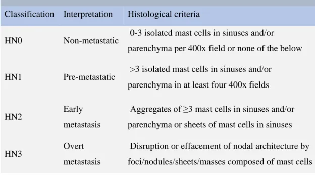
Table 2. Nodal metastasis classification
Lymph node metastasis classification system
Classification Interpretation Histological criteria
HN0 Non-metastatic 0-3 isolated mast cells in sinuses and/or
parenchyma per 400x field or none of the below
HN1 Pre-metastatic >3 isolated mast cells in sinuses and/or parenchyma in at least four 400x fields
HN2 Early
metastasis
Aggregates of ≥3 mast cells in sinuses and/or parenchyma or sheets of mast cells in sinuses
HN3 Overt
metastasis
Disruption or effacement of nodal architecture by foci/nodules/sheets/masses composed of mast cells
Stage III cMCTs may have multiple masses due to the development of multiple de novo masses. Stage IV is difficulted by challenges in clinical detection of distant metastasis and lack of post-mortem examination of dogs. Some studies suggest the advantage of liver and spleen ultrasound-guided aspiration in early detection of distant metastasis, even in the absence of abdominal alterations (56,65).
19
II. Research Project
3.
Aim
Currently, tumour grade is the most valuable predictor of cMCT biological behaviour. Histological grading evaluates malignancy severity and labels tumours based on morphological features. The qualitative and subjective nature of tumour grading is highly sensitive to personal bias, causing significant intra and inter-observer variability and consequent poor reproducibility. Additionally, tumour grade has a crucial impact on prognosis and patient treatment, reinforcing the need to substitute subjective and qualitative parameters by objective and quantitative techniques. The goal of this study was to:
a) Objectively quantify cMCT nuclear size with a stereological approach b) Investigate VV‘s relation with tumour grade
20
4.
Materials & Methods
4.1. Case selection and histopathological analysis
The pathology archives of DnaTech were used to select 55 cMCTs from December 2016 to December 2017. Exclusion criteria included absence of an identifiable vertical-axis, incisional biopsies and end-stage disease. Data regarding age, sex and breed was not included.
All cMCTs were formalin-fixed and paraffin-embedded at the time of submission. Each specimen was sectioned perpendicularly to the cutaneous surface into 5-µm-thick sections and routinely H&E-stained. These tumours were blindly graded following Patnaik and Kiupel by three pathologists. The final grade corresponded to the grade assigned by at least two of the three pathologists (66).
4.2. Outcomes
Considering that the use of different treatment modalities would have influenced the interpretation of results, only cMCTs treated with surgical removal alone were selected for prognostic analysis (n = 31) (67). Veterinarians were surveyed regarding clinical outcomes including local recurrence, lymph node metastasis and disease-related death. Animals were followed until May 2019 with a minimum follow-up of one year. Histopathological confirmation of nodal metastasis was performed when possible. Distant nodules were considered de novo cMCTs and excluded from statistical analysis (38). Surgical margins were also evaluated.
4.3. Stereological estimations
Each slide was scanned with HAMAMATSU NanoZoomer-SQ Digital slide scanner C13140-01 and the fields of 800X magnification were assessed with NDPI view software. Cross-sections were rotated along their vertical axis, so the cutaneous surface was positioned upwards.
21
4.3.1. Field selection
The distance between fields was approximately constant and proportional to the overall tumour sectional area, visible on the map widget on the lower right-hand corner (Figure 8). The final magnification (M) was calculated dividing the tissue scale on page (12.4 cm = 124000 µm) by the tissue scale on tissue level (50 µm) (Equation 2) (3).
Equation 2.M = 𝑆𝑐𝑎𝑙𝑒 𝑙𝑒𝑛𝑔𝑡ℎ 𝑜𝑛 𝑝𝑎𝑔𝑒 (𝜇𝑚)
𝑆𝑐𝑎𝑙𝑒 𝑙𝑒𝑛𝑔𝑡ℎ 𝑎𝑡 𝑡𝑖𝑠𝑠𝑢𝑒 𝑙𝑒𝑣𝑒𝑙 (𝜇𝑚) =
124000(𝜇𝑚)
50 (𝜇𝑚) = 2480X
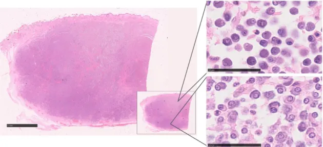
Figure 9. Selection of fields. Cutaneous mast cell tumour (cMCT), H&E, Bar 5 mm in
overview, bars 50 µm in inserts.
4.3.2. Measurements
An orientation frame was taped onto the screen (Figure 10). The first field had a direction determined by a randomly generated number between 1 and 97, in this case, 20 (outlined in red) (Figure 11). The following orientation numbers were systematically determined by the addition of 37 – (Table 2).
22
Figure 10. Orientation frame. cMCT, H&E, Bar 50 µm
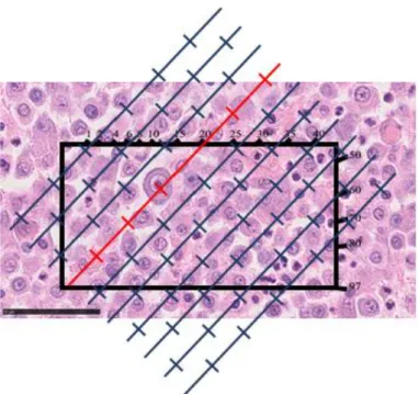
Figure 11. Orientation frame + Test-lines. cMCT, H&E, Bar, 50 µm
Table 3
. Orientation numbers
1 38 75 15 52 89 29 66 6 43 80 20 57 94 34 71 11 48 85 25 62 2 2 39 76 16 53 90 30 67 7 44 81 21 58 95 35 72 12 49 86 26 63 3 3 40 77 17 54 91 31 68 8 45 82 22 59 96 36 73 13 50 87 27 64 4 4 41 78 18 55 92 32 69 9 46 83 23 60 97 37 74 14 51 88 28 65 5 5 42 79 19 56 93 33 70 10 47 84 24 61 1
23
The orientation frame also served as a counting frame. The top and right-hand corner lines were defined as inclusion lines, whereas the bottom and left-land lines were defined as exclusion lines. Figure 12 exemplifies nuclei point-sampling, outlined in red.
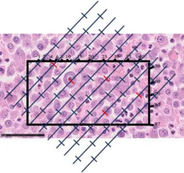
Figure 12. Nuclei point-sampling. cMCT, H&E, Bar, 50 µm
Each point-sampled nucleus landing partially or within the orientation frame was measured with a logarithmic ruler of 3.35 cm. Each nuclear intercept was measured from nuclear boundary to nuclear boundary in the direction of the test-lines. Figure 13 illustrates an example of an intercept falling into the ruler’s first class (outlined in green). Intercept measurement was registered along a minimum of 10 fields of view. The frequency of each class along the fields of view is used in VV calculations.
24
Figure 13. Intercept length measurement. cMCT, H&E, Bar, 50 µm
4.3.3. Calculations
Table 4 reflects the general formulas applied in VV estimation. Column A indicates each
class of the logarithmic ruler. The length of each class (Column B) is estimated by computing the upper limit of class z (1, 2… n-1, n) in a ruler of n classes (n = 15) of length Ln. If Ln=3.35 cm, the upper limit of class 1 is 0.62 cm (Equation 3) (15,19).
Equation 3.Upper limit of class 1 = (𝐿𝑛) 3 10𝑛/(𝑛−1)−1×(10 𝑧/(𝑛−1)− 1) = = 3.35 3 1015/(14)−1×(10 1/(14)− 1) = 0.62 cm
25
Table 4. Example of general formulas applied in mean nuclear volume (VV) estimations
(adapted from Sorensen 1991b, Skau et al. 2001). VV formulas A B C D E F G Class no. Upper Limit Length (cm) Upper Limit Length³ (cm³) Class Width Length³ (cm³) Class mid-volume³ (cm³) Observed no. per class E x F 1 0.85 0.62 0.62 0.27 12 3.76 2 1.11 1.36 0.73 0.99 14 13.86 3 1.31 2.22 0.87 1.79 8 14.32 4 1.48 3.24 1.02 2.73 9 24.60 5 1.64 4.45 1.2 3.84 4 15.38 6 1.8 5.86 1.42 5.16 3 15.47 7 1.96 7.54 1.67 6.70 0 0 8 2.12 9.51 1.97 8.52 0 0 9 2.28 11.83 2.32 10.67 0 0 10 2.44 14.57 2.74 13.20 0 0 11 2.61 17.79 3.23 16.18 0 0 12 2.78 21.6 3.8 19.69 0 0 13 2.97 26.08 4.48 23.84 0 0 14 3.15 31.37 5.29 28.72 0 0 15 3.35 37.6 6.23 34.48 0 0 ∑ 50 87.39
Column C represents the upper limit of each class raised to the third power (length³). Column D is the class width in terms of length³, given by the difference between the volume (Column C) of one class and the preceding class (example: class 3 = 3.24 - 2.22 = 1.02). Column E is the upper limit of a class minus half the class width (Column C-Column D/2). C-Column F exhibits the frequency of each class. C-Column G indicates the
26
sum of the intercept lengths (l03) (adapted from 44,45). Following the measurement of a minimum of 50 cells per specimen, the mean intercept length is given by Equation 4.
Equation 4. 𝑙̅ = 03 ∑𝐺
∑𝐹 = 86.85
50 = 1.75 cm³
The final magnification (2480X) and the length of the ruler are required to convert mm³ to µm³ (Equation 5). Equation 5. VV = 𝜋 3×( 𝐿₁₅ × 10000 3 × 𝑀 ) 3 × 𝑙̅ = 03 𝜋 3 ×( 3.35 × 10000 3 × 2480 ) 3 ×1.74 = 167.5 µm³ 4.4. Statistical analysis
Statistical analysis was conducted using Excel, GraphPad and R with ggplot2 and pROC packages (68,69). The interobserver agreement of histological grading was investigated using Fleiss’s Kappa statistics (70). Wilcoxon’s rank-sum test was used to test differences in VV values according to tumour grade. VV values were converted into a
dichotomous variable, according to Patnaik’s and Kiupel’s grading scheme, G2 or G3 cMCTs and LG or HG cMCTs, respectively. Tumours treated with surgery alone were given an outcome value of zero (OC0). Outcome of one (OC1) included animals manifesting local recurrence, lymph node metastasis and death associated with disease. Wilcoxon’s rank-sum test was used to test differences in VV and surgical margins
according to outcome. Receiver Operating Characteristics (ROC) curve analysis was used to access the prognostic value of VV. ROC curves plotting the sensitivity (true
positive rate) against 1-specificity (false positive rate) were generated and the areas under the curves (AUC) were calculated.
27
5.
Results
5.1. Histological grading
The final grades had at least two similar grades assigned by the three pathologists. Overall, LG were graded as G2, and HG were graded as G3 (Figure 14).
Figure 14. Grading distribution
The next step was the evaluation of interobserver variability of tumour grade. The 55 cMCTs analysed resulted in a total of 0 G1, 39 G2 and 16 G3 (Table 5). The three pathologists attributed the same grade in 47.3% (n = 26) of the cases. G2 had the highest disagreement rates (Table 6). The Kappa value (κ) was 0.32 (P < 0.05).
Table 5. Patnaik grading distribution
Patnaik grading Observer G1 G2 G3 1 0 32 23 2 11 33 11 3 2 37 16 Final grade 0 39 16
28
Table 6. Patnaik agreement rates
Patnaik agreement
Grade n Agreement Disagreement
G2 39 17 (43.6%) 22 (56.4%)
G3 16 9 (56.25%) 7 (43.75%)
∑ 55 26 (47.3%) 29 (52.8%)
35 cMCTs were graded as Kiupel’s LG and 20 tumours were graded as HG (Table 7). The three pathologists attributed the same grade in 61.8% (n = 34) of the cases. HG had the highest disagreement rates (Table 8). The Kappa value (κ) was 0.46 (P < 0.05).
Table 7. Kiupel grading distribution
Kiupel grading Observer LG HG 1 31 24 2 33 22 3 38 17 Final grade 35 20
Table 8. Kiupel agreement rates
Kiupel agreement
Grade n Agreement Disagreement
LG 35 23 (65.7%) 12 (34.3%)
HG 20 11 (55%) 9 (45%)
29
5.2. VV
The measurement of 58 point-sampled intercepts on average took approximately 15 minutes per tumour. VV values ranged from 50.05 to 495.05 µm³. Table 9 and 10 illustrate
VV values according to tumour grade. VV had similar results in G2 (VV = 145.63 ± 38.57
µm³) and LG (VV = 139.58 ± 35.19 µm³), as well as in G3 (VV = 228.98 ± 88.60 µm³)
and HG (VV = 222.89 ± 80.34 µm³). G3 and HG cMCTs had VV greater than 200 µm³
more frequently.
Table 9. Patnaik VV values descriptive statistics
VV (µm³) according to Patnaik grading
Results G2 G3 Mean 145.63 228.98 SD 38.57 88.60 Median 150.70 212.06 Maximum 222.72 495.99 Minimum 50.05 131.11
Table 10. Kiupel VV values descriptive statistics
VV (µm³) according to Kiupel grading
Results LG HG Mean 139.58 222.89 SD 35.19 80.34 Median 145.07 208.56 Maximum 208.95 495.99 Mininum 50.05 131.11
5.2.1. Wilcoxon rank-sum test
Differences in VV values according to tumour grade were tested using the
30
significant between G2 and G3 median values (P < 0.05), as well as between LG and HG (P < 0.05) (Charts 1a and 1b).
Chart 1a. VV (MNV) vs Patnaik Wilcoxon’s rank-sum test
Chart 2b. VV (MNV) vs Kiupel Wilcoxon’s rank-sum test
5.2.2. ROC curve
Receiving Operating Characteristic (ROC) curve was used to evaluate the discriminative power of VV between grades. The area under the curve (AUC) was 0.86
(95% CI 0.75-0.97) in Patnaik grading. A cut-off value for G3 of VV > 174 µm³ is
provided with 82.1% specificity (proportion of correctly identified negative observations) and 75.0% sensitivity (proportion of correctly identified positive observations) (Chart 2a). In Kiupel grading the AUC was 0.90 (95% CI 0.82-0.99). The cut-off value for HG was VV > 173.7 µm³ and had 88.6% specificity and 80.0%
31
Chart 3a. VV (MNV) vs Patnaik ROC curve.
Chart 4b. VV (MNV) vs Kiupel ROC curve
5.3. Outcomes
Table 11 reflects tumour grades of dogs treated after surgery (OC0 – n = 23) and dogs with progression of disease (OC1 – n = 8). The latter revealed either local recurrence (n = 5), regional lymph node metastasis (n = 3) or death related to disease (n = 7). Dogs treated after surgery were graded as G2/LG, except for one tumour graded as G3/HG. Dogs of OC1 had tumours of all 4 grades.
Table 11. Outcome and tumour grade assignment
Outcome results OC0 (n = 23) Patnaik 22 G2 1 G3 Kiupel 22 LG 1 HG OC1 (n = 8) Patnaik 4 G2 4 G3 Kiupel 2 LG 6 HG
32
Table 13 reflects VV of cMCTs treated with surgical removal only. The mean (± SD) was
VV = 148.48 µm³ (± 36.33 µm³) in dogs of OC0 and VV = 198.87 µm³ (± 47.88 µm³) in
dogs of OC1 (Table 12).
Table 12. Outcome VV values descriptive statistics
VV (µm³) according to outcome
Results OC0 OC1
Mean 148.48 198.87
SD 36.33 47.88
Median 150.70 176.59
Maximum 242.26 297.63
Minimum 76.25 152.76
Wilcoxon rank-sum test revealed significant difference (P = 0.002) between VV values
of different outcomes (Chart 3). A ROC curve analysed the discriminating power of VV
estimations between surgically treated cMCTs and those revealing progression (AUC = 0.86, 95% CI 0.72-0.99). A cut-off value for OC1 of VV > 167.7 µm³ is provided with
78.3% specificity and 87.5% sensitivity (Chart 4).
Tumours that recurred and/or metastasized (OC1) had VV > 152 µm³. These included a
4 G2 (VV = 152, 174, 179 and 209 µm³) and 2 LG (VV = 152 and 209 µm³). Also, one
G3/HG (VV = 242 µm³) was treated after surgical removal alone (OC0). The small
number of animals with progression of disease may have influenced these results, however, these results suggest that cMCT VV values are divided into two groups
independent of tumour grade: 1) VV < 152 µm³ - cMCTs of benign behaviour; 2) VV >
33
Chart 5. VV vs Outcome Wilcoxon’s rank-sum test
34
Table 13 represents surgical margins’ descriptive statistics. Wilcoxon rank-sum test revealed differences between margins of OC0 and OC1 were not significant (P > 0.05) (Chart 5).
Table 13. Surgical margins descriptive statistics
Chart 7. Surgical margins (cm) vs OC Wilcoxon’s rank-sum test
Surgical margins (cm) OC0 Mean 0.9478 SD 0.842 Median 0.6 Maximum 3 Minimum 0.2 OC1 Mean 0.775 SD 0.8648 Median 1 Maximum 2 Minimum 0
35
6.
Discussion
The purpose of this study was to evaluate the prognostic significance of VV in cMCTs.
VV was compared with tumour grade and outcome results and when cut-off values were
established, higher grading and likelihood of progression of disease revealed close VV
values (VV > 174 µm³ and 168 µm³, respectively).
Histological grading was evaluated from both microscopical and digital slides. Some slides were affected by scanning, which may have contributed to interobserver variability. Patnaik grading had a fair statistical concordance among the three pathologists (κ= 0.32) (71). In this case, the final grade was based on the one assigned by at least two pathologists. The final grades did not include G1, however, some tumours (n = 13) had a classification of G1 assigned by one pathologist. All three pathologists agreed in the diagnosis of only 43.6% G2 (17 out of 39). Patnaik grading scheme is based on cellularity, mast cell differentiation, granulation, location and mitotic count. One study suggests that association of this system with low agreement rates in G1 and G2 may be due to intratumoral heterogeneity, subjective criteria, or even inability to distinguish or determine grade characteristics (72). This ambiguity is associated with the location of the tumour - G1 is confined to the dermis and G2 extends to the subcutis. Some studies also found lack of differences in survival time between the latter (42,45). There is some evidence that in a situation where a tumour is borderline between G1 and G2, pathologists tend to opt for G2 (45). One study found no association between tumour depth and prognosis, reinforcing the need to reformulate cMCT grading scheme (73). A higher agreement rate in the assignment of G3 was expected. Only 56.25% of the tumours were diagnosed as G3 by the three pathologists (9 out of 16). One possible explanation for the low agreement is the mitotic count of G3, which includes tumours with 3 to 6 mitotic figures per hpf. cMCTs have relatively low mitotic counts and there is evidence that based on this criterion alone, a lot of G3 would not be graded as such (45).
Kiupel grading had a moderate statistical concordance among the three pathologists (κ = 0.46) (71). Kiupel grading is based on cellular atypia, mitotic count and number of multinucleated cells in 10 hpf. 23 out of 35 were diagnosed as LG by the three pathologists, corresponding to 65.7%. Only 55% of the tumours had consistent assignment of HG (11 out of 20). These results agree with association of this grading scheme with greater consistency than Patnaik grading (42,45,46,66), however, one
36
possible explanation to the observed variability is the subjectivity associated with the selection of fields based on higher mitotic activity and karyomegaly.
Wilcoxon sum-rank’s test revealed statistical differences between G2 and G3 VV median
values (P = < 0.05), as well as LG and HG (P < 0.05). Apart from 4 G2 graded as HG, G2 corresponded to LG, as well as G3 and HG. These groups also had close median VV
values. Patnaik grading had moderately accurate discriminative power between G2 vs G3 (AUC = 0.86). Kiupel grading, on the other hand, indicated highly accurate discriminative power between LG and HG (AUC = 0.90) (74). These results agreed with previous studies suggesting the superior prognostic value of Kiupel grading (42,45,46,66). Despite the greater specificity and sensibility in Kiupel grading, the cut-off values provided for G3 and HG are similar (VV > 173,8 µm³ and VV > 173,7 µm³, respectively).
Follow-up data was collected from medical histories, which may have added a source of bias to this study. Local recurrence, nodal metastasis and death related to disease were the main criteria used for evaluation of cMCT malignancy. We were not able to accurately evaluate lymph node metastasis by histopathology in all animals - some animals had only suspected lymph node involvement due to clinical enlargement. Also, information regarding survival time or progression-free interval was unavailable for some tumours. Regardless, 7 out of 8 animals died or were euthanised due to clinical signs related to cMCT disease. The remaining dog had local recurrence. Additionally, statistical analysis revealed that surgical margins did not significantly interfere with the progression of disease (P > 0.05).
The discriminative power of VV between tumours of benign behaviour (OC0) and
tumours with progression of disease (OC1) was moderately accurate (AUC = 0.86). A small number of G2/LG is included in OC1, which agrees with evidence of a need to monitor LG, since a small number tends to recur and/or metastasise (42). A cut-off value for tumours with OC1 is provided (VV > 168 µm³). Despite the similarity observed
between the latter and tumour grade’s cut-off values, there was some overlap between OC0 and OC1 VV values. These results suggest that greater VV values are associated with
worse prognosis, however, the small number of animals with progression of disease may have influenced these results. A larger study is required to confirm these preliminary results.
37
Due to the retrospective nature of this study, VV was estimated in approximately VUR
sections from previously embedded cutaneous biopsies. The selection of fields was performed so at least 50 intercepts were measured per tumour. For efficiency reasons, fields demonstrating mostly areas of necrosis and collagen fibres were disregarded. The map widget available on NDPI view software permitted a standardization of the selection of fields, as well as an even distribution of fields proportional to the cross-sectional area. However, the reproducibility of VV is related to the little effect of the lowest sampling
levels, such as differences between fields of view or the precision of each measurement.
One study even found that a subjective selection of fields of areas showing greater atypia had little interference in breast cancer VV, suggesting that this technique does not require
great histopathology experience from the operator (75). The greatest impact on VV
estimations is due to biological differences between patients (10).
VV estimation owes much of its strength to the fact that it combines information about
tumour size and its variation (76). Regarding that this is a volume-weighted estimation, size is favoured, and larger nuclei have thus greater influence in the final value. VV also
provides information about pleomorphism, one of the most dominant features when it comes to tumour grading. VV also provides knowledge of three-dimensional nuclear size
with no assumptions about shape, one of the most elusive structures to quantify (10). Lastly, is a quick and inexpensive technique applicable to routine histopathology.
In relation to the absolute VV values observed in this study, they ranged between 50 µm³
to 496 µm³. These are similar to previous estimations of VV in human tumours such as
ductal carcinoma of the breast (103 – 734 µm³), lobular carcinoma of the breast (115 - 301 µm³) or cutaneous malignant melanoma (99 – 466 µm³) (10,25,26). Regardless, this study provides the first cMCT VV estimation, therefore the reproducibility of the provided
estimations needs to be investigated. This study found a close association between VV
and tumour grade, suggesting that VV provides an unbiased and objective means of
diagnosis of G3/HG cMCTs. In the future, additional studies including a larger number of animals demonstrating progression of disease are needed to validate these preliminary studies. It is also necessary to evaluate VV of other MCTs, such as subcutaneous MCTs
or MCTs located at mucous membranes, in order to investigate if VV is influenced by
38
7.
Conclusion
The stereological estimation of VV is a simple and quick technique, easily applied in
routine histopathology with no extra equipment or cost. The manual estimation takes about 15 minutes per tumour and provides reproducible information about nuclear size. This study provides evidence of the prognostic value of VV in canine mast cell tumours.
These preliminary results suggest that VV may objectively improve the early detection of
G3/HG cMCTs with a cut-off value of VV > 174 µm³. A study involving a larger number