Universidade de Lisboa
Faculdade de Ciˆ
encias
Departamento de Estat´ıstica e Investiga¸c˜
ao Operacional
Study of the Role of SETD2
Mutations in clear cell Renal Cell
Carcinoma (ccRCC)
Catarina Faria de Almeida
Trabalho de Projecto
Mestrado em Bioestat´ıstica
2013
Universidade de Lisboa
Faculdade de Ciˆ
encias
Departamento de Estat´ıstica e Investiga¸c˜
ao Operacional
Study of the Role of SETD2
Mutations in clear cell Renal Cell
Carcinoma (ccRCC)
Catarina Faria de Almeida
Trabalho de Projecto
Mestrado em Bioestat´ıstica
Trabalho de projecto orientado por Professora Doutora Lisete Maria Ribeiro de Sousa e por Professora Doutora Ana Rita Fialho Grosso
aaaaa
aaaaa
Acknowledgements
To my great tutors, Professor Lisete Sousa and Professor Ana Rita Grosso, I have to express sincere gratitude, if there are people that can complain about their tutors, I was definitely not one of them, always teaching, always helpful, always patient, always supportive, always kind, even when working with me was not easy.
A special thank you to Jo˜ao, who was a source of stability that he can not possibly imagine, thanks for all you’ve done.
To Ana who is always ready to step in, always somebody to lean on. To my sister Mariana and to Sofia, always so close, no matter how far.
Last and most dear to my heart, I wish to thank my parents, who my nerves and anxiety tried to push away, and they never allowed for that to happen, you’ve been so good to me. I subscribe the sincere clich´e that I owe them everything.
To all of these and to everyone who stood by my side and helped me get to where I am today, a sincere thank you. Catarina Almeida, September 2013
aaaaa
Abstract
Clear cell Renal Cell Carcinoma, ccRCC, is the most common form of Renal Cancer, accounting for 90% of these cancers cases. It is well estab-lished that the majority of these cancers happen when both alleles of VHL (Von Hippel Lindau) tumour suppressor gene are mutated. It has also been observed that patients with this form of cancer present mutations on the SETD2 gene which applies its functions during transcription.
In the last few years the growth within sequencing technologies has been astonishing. Next Generation Sequencing technology, NGS, provides tools for assessing full genomes to a reference sequence in a matter of days, being extremely accurate, while also increasingly cost effective. One of its many applications is RNA-Sequencing, a method for transcriptome analysis.
Throughout this thesis we aimed at analysing RNA-Seq data from six samples: four with mutations on the SETD2 gene and two control samples. The main goal was to understand how the remaining genes on the transcrip-tome respond to these genes mutations.
In the first part of this work we aimed at analysing several forms to normalize the data, resorting to R software packages (EDASeq, DESeq and edgeR). Data normalization is a crucial step on NGS techniques, as these techniques have some inherent bias that need to be accounted for. DESeq proved to be the most selective, while EDASeq is not as stringent. The second part of this work aimed at identifying differentially expressed genes, to infer which genes behave in a significant way in the samples, packages edgeR, DESeq and RankProd. We identified six new genes as differentially expressed. Keywords: Next Generation Sequencing (NGS), clear cell Renal Cell Carcinoma, normalization, differential expression, SETD2
aaaaa
Resumo
O carcinoma renal de c´elulas claras, ccRCC, ´e o tipo mais comum de can-cro renal, sendo respons´avel por cerca de 70% destes tumores, com a mais alta taxa de mortalidade entre todos os tipos de cancro renal. A grande maio-ria destes tumores deve-se a muta¸c˜oes no gene VHL, um gene supressor de cancro. N˜ao obstante, v´arios estudos de sequencia¸c˜ao do ccRCC acabaram por revelar a ocorrˆencia de muta¸c˜oes som´aticas no gene SETD2, uma Histone methyltransferase que trimetila a lisina 36 na histona H3 (H3K36me3). Este gene tem um papel fundamental na transcri¸c˜ao, um dos principais passos na express˜ao gen´etica – processo pelo qual s˜ao geradas prote´ınas perfeita-mente funcionais, permitindo que o ADN se desenrole e seja posteriorperfeita-mente transcrito. Est´a localizado no bra¸co curto do cromossoma 3 e as muta¸c˜oes deste gene conduzem `a perda de fun¸c˜oes deste mesmo cromossoma.
O objectivo biol´ogico da presente tese ´e avaliar as altera¸c˜oes do transcrip-toma, induzidas pelas muta¸c˜oes no gene SETD2. Esta quest˜ao ser´a abordada utilizando dados do transcriptoma completo, de linhas celulares mutadas no gene SETD2 e de linhas celulares n˜ao mutadas do gene wild tipe (WT), no ccRCC. Os dados desta an´alise consideraram 4 amostras biol´ogicas de transcriptomas mutados do genoma SETD2 e 2 amostras wild tipe, dados estes que foram gerados pela unidade do investigador S´ergio Almeida, do Instituto de Medicina Molecular (IMM da FMUL).
Recentemente, o desenvolvimento de novas tecnologias de m´etodos de sequencia¸c˜ao, designadas por Next Generation Sequencing (NGS), disponi-bilizou um novo m´etodo que, em simultˆaneo, executa o mapeamento e a quantifica¸c˜ao de transcriptomas, chamado sequencia¸c˜ao de RNA (RNA-seq). Apesar de mais expendioso do que os estudos de microarrays e ainda com alguns problemas de an´alise de dados por resolver, a sequencia¸c˜ao do RNA pode avaliar o transcriptoma completo, disponibilizando a derradeira solu¸c˜ao para a an´alise dos n´ıveis e da estrutura de transcriptomas processados e n˜ao processados, sob diferentes condi¸c˜oes. Esta t´ecnica disponibiliza uma impor-tante poupan¸ca de tempo (o genoma humano completo pode ser sequenciado em menos de uma semana, dependendo das op¸c˜oes do investigador) com qualidade, precis˜ao de leitura (cerca de 98%) e poupan¸cas de tempo. O transcriptoma completo de cada amostra ´e convertido em cRNA e separado em pequenos fragmentos (cerca de 200, 300nt), estes fragmentos s˜ao
poste-riormente utilizados como modelos no passo de sequencia¸c˜ao, onde s´o uma pequena sequˆencia da parte final do fragmento ir´a ser sequenciada (chamada de read ). Este processo gera milh˜oes de reads, que podem ser depois al-inhadas com o genoma e originar uma tabela de contagens para cada gene (n´umero de reads, por gene) por amostra.
Algumas ferramentas bioinform´aticas foram recentemente desenvolvidas, para analisar esta imensa informa¸c˜ao gerada pela t´ecnica RNA-seq. Estas ferramentas diferem entre si quanto `a normaliza¸c˜ao e `as t´ecnicas estat´ısticas aplicadas, com impacto nos resultados finais. Assim, o objectivo da pre-sente tese ´e explorar e comparar os diferentes m´etodos aplicados ao prob-lema biol´ogico acima mencionado. Para o efeito, a nossa an´alise recorreu ao Bioconductor. O Bioconductor ´e um software de utiliza¸c˜ao gratuita, n˜ao impondo quaisquer licen¸cas de utiliza¸c˜ao, que disponibiliza c´odigo aberto para Bioinform´atica. Aqui, encontram-se packages que permitem processar a informa¸c˜ao no que respeita aos 2 passos da an´alise: normaliza¸c˜ao e an´alise da express˜ao diferencial dos genes. O trabalho desta tese foi desenvolvido considerando a an´alise dividida nestes dois passos principiais: normaliza¸c˜ao e express˜ao diferencial. Os nossos estudos ir˜ao ser desenvolvidos em torno das diferentes formas de normaliza¸c˜ao dos dados, analisando posteriormente os diferentes resultados que se obtiveram na express˜ao diferencial dos dados. A normaliza¸c˜ao ´e o passo pelo qual se consegue que uma base de dados com contagens profundamente discrepantes entre si possa ser compar´avel, aplicando a estes dados um denominador comum que toma em considera¸c˜ao os erros associados `a utiliza¸c˜ao desta t´ecnica. A express˜ao diferencial ´e o passo onde se identificaram os genes que revelaram significativas altera¸c˜oes da express˜ao estat´ıstica, entre duas amostras, tal como a muta¸c˜ao do gene SETD2 e as linhas das c´elulas do ccRCC wild type. No essencial, isto significa que estes genes revelam uma altera¸c˜ao significativa da sua express˜ao, das amostras mutadas para as wild type.
A nossa an´alise baseou-se na utiliza¸c˜ao de 4 packages, EDASeq, edgeR, DESeq e RankProd. Enquanto o primeiro foi desenhado apenas para realizar a normaliza¸c˜ao, o ´ultimo foca-se apenas na an´alise da express˜ao diferen-cial. Ambos os packages edgeR e DESeq possuem abordagens pr´oprias para realizar ambos os passos, podendo ao mesmo tempo receber contagens de dados normalizados pelo EDASeq. O m´etodo RankProd pode receber dados normalizados pelos m´etodos EDASeq e DESeq, e o m´etodo edgeR tamb´em pode receber dados normalizados obtidos pelo m´etodo DESeq.
A forma como estes dados s˜ao normalizados vai depender das premis-sas que cada m´etodo utiliza para normalizar os dados: o edgeR e o DESeq consideram abordagens diferentes na normaliza¸c˜ao between lane, enquanto o m´etodo EDASeq realiza uma normaliza¸c˜ao na pr´opria lane relativamente
ao conte´udo em GC, antes de proceder `a normaliza¸c˜ao textitbetween lanes. Observ´amos ainda que todas estas abordagens disponibilizam bons n´ıveis de normaliza¸c˜ao, bem correlacionados entre si (obtendo valores de 0.98/1.00 no coeficiente de correla¸c˜ao de Pearson) e no que respeita aos dados em bruto.
As combina¸c˜oes estudadas entre os v´arios m´etodos tiveram o objectivo de permitir uma compara¸c˜ao detalhada das metodologias, no que respeita aos seus pr´oprios protocolos (normaliza¸c˜ao DESeq combinada com a an´alise de ex-press˜ao diferencial com DESeq e normaliza¸c˜ao edgeR combinada com a an´alise da express˜ao diferencial com edgeR) e `a jun¸c˜ao de protocolos: nomeadamente as diferentes abordagens no passo da normaliza¸c˜ao pelos m´etodos - EDASeq ou DESeq – e ainda as diferentes abordagens no passo da express˜ao diferencial dos m´etodos – edgeR, DESeq ou RankProd.
No que respeita a protocolos pr´oprios, observ´amos que o protocolo com-pleto do m´etodo edgeR identificou muito mais genes que o m´etodo DESeq, independentemente dos n´ıveis de significˆancia considerados (1%, 5% e 10%). No que respeita `a jun¸c˜ao de protocolos, quando se juntou a normaliza¸c˜ao do EDASeq `a express˜ao diferencial do edgeR, obteve-se um n´umero significativa-mente maior de genes identificados quando comparado com quaisquer outros m´etodos.
O m´etodo RankProd acabou por apresentar uma nova perspectiva sobre os dados, tendo sido concebido para trabalhar os dados numa l´ogica de microar-rays; contudo, ao assumir que cada lane dos nossos dados funciona como um array, propusemo-nos investigar se este package se podia ajustar aos nossos dados de NGS. Observ´amos que o RankProd se ajustava adequadamente ao receber dados normalizados oriundos do m´etodo DESeq, mas falhava quando recebia dados normalizados pelo m´etodo EDASeq.
Observ´amos que, globalmente, o m´etodo DESeq, quando utilizado como processo de normaliza¸c˜ao, conduz `a identifica¸c˜ao de um n´umero menor de genes diferencialmente expressos que o EDASeq, para todos os n´ıveis de sig-nificˆancia considerados (1%, 5% e 10%). Por outro lado, quando considera-dos toconsidera-dos os m´etodos para a express˜ao diferencial, detect´amos que o m´etodo edgeR identificou mais genes que o RankProd ou o DESeq, para os mesmos n´ıveis de significˆancia.
Observ´amos ainda que a maioria dos genes identificados com estes m´etodos (com excep¸c˜ao dos procedimentos de normaliza¸c˜ao do EDASeq) conduziram a um maior n´umero de contagens para genes up regulated que para genes down regulated, o que significa que estes genes demonstram possuir maior ex-press˜ao diferencial quando mutados do que nas amostras wt. O passo seguinte na an´alise foi perceber se os genes que estes m´etodos identificam como dife-rencialmente expressos s˜ao os mesmos. Considerando todos os m´etodos do R, identific´amos 6 genes diferencialmente expressos comuns a todos eles (para
uma FDR=5%): ”SLC2A10”, ”COL14A1”, ”GPR173”, ”LOC100506178”, ”EREG” e ”ADAMTSL1”. Uma vez exclu´ıdo o RankProd desta compara¸c˜ao, foram identificados 27 genes como diferencialmente expressos, considerando o mesmo valor para a FDR.
Considerando investiga¸c˜oes futuras, e no que respeita aos resultados obti-dos pelo Bioconductor, a combina¸c˜ao entre t´ecnicas que revelou um maior n´umero de genes com express˜ao diferencial ´e entre o m´etodo EDASeq para a normaliza¸c˜ao com o m´etodo edgeR para a an´alise da express˜ao diferencial.
Adicionalmente, todas as combina¸c˜oes de t´ecnicas onde o m´etodo EDASeq executa a normaliza¸c˜ao, claramente resultaram em amostras com um maior n´umero de contagens.
No princ´ıpio deste projecto, propusemo-nos estudar 6 amostras de transcriptoma, obtidas com o RNA-Seq, duas correspondendo a amostras controlo, as outras quatro apresentando muta¸c˜oes no gene SETD2, o que leva `
a ocorrˆencia do ccRCC. O desafio foi analisar os dados, procurando identi-ficar genes que reagissem `as muta¸c˜oes do SETD2, respondendo `a quest˜ao de como este gene afecta os restantes genes no transcriptoma. Outro de-safio a que nos propusemos, conforme indicado neste texto, foi a compara¸c˜ao de metodologias por forma a melhor aferir sobre o objectivo prim´ario deste trabalho.
Este trabalho permitiu identificar 6 novos genes que respondem `as muta¸c˜oes do SETD2.
Palavras chave: Next Generation Sequencing, clear cell Renal Cell Carcinoma, normaliza¸c˜ao, Express˜ao diferencial, SETD2
Contents
Acknowledgments i
Abstract iii
Resumo v
List of Figures xiv
List of Tables xv
Preface xvii
1 Biological Background 1
1.1 Genetics . . . 1
1.2 clear cell Renal Cell Carcinoma (ccRCC) . . . 4
1.3 Next Generation Sequencing (NGS) . . . 7
1.4 Objectives . . . 9
2 Methods for data Analysis 11 2.1 NGS data analysis workflow . . . 11
2.2 Methods for Normalization . . . 15
2.2.1 edgeR . . . 16
2.2.2 DESeq . . . 17
2.2.3 EDASeq . . . 18
2.3 Methods for Differential Expression Gene analysis . 20 2.3.1 edgeR . . . 21
2.3.2 DESeq . . . 23
2.3.3 RankProd . . . 25
3 Results 29 3.1 Samples . . . 29
Table of Contents
3.2 Normalization . . . 31
3.2.1 edgeR . . . 31
3.2.2 DESeq . . . 32
3.2.3 EDASeq . . . 33
3.3 Differential Expression Analysis . . . 39
3.3.1 edgeR . . . 39 3.3.2 DESeq . . . 47 3.3.3 RankProd . . . 53 3.4 Comparing methodologies . . . 56 4 Discussion 65 References 67
List of Figures
1.1 Chromosome . . . 3
1.2 Gene Expression mechanism . . . 5
1.3 Urinary tract System . . . 6
1.4 NGS Genome Analyzer . . . 9
2.1 RNA-sequencing workflow . . . 12
2.2 NGS pipeline . . . 13
3.1 ccRCC samples . . . 30
3.2 Biasplots representing EDASeq effect on normalization 35 3.3 Boxplot representing EDASeq offset effect on normal-ization . . . 37
3.4 Boxplots of all methods normalization effect . . . . 38
3.5 Normalization with edgeR and DE analysis with edgeR – MDS Plot . . . 39
3.6 Normalization with edgeR and DE analysis with edgeR – dispersion plot . . . 41
3.7 Normalization with edgeR and DE analysis with edgeR – plot of all genes identified as DE . . . 42
3.8 Normalization with EDSeq and DE analysis with edgeR – MDS Plot . . . 43
3.9 Normalization with EDASeq and DE analysis with edgeR – dispersion plot . . . 44
3.10 Normalization with EDASeq and DE analysis with edgeR – plot of all genes identified as DE . . . 45
3.11 Normalization withDESeq and DE analysis with edgeR – MDS Plot . . . 46
3.12 Normalization withDESeq and DE analysis with edgeR – dispersion plot . . . 47
3.13 Normalization withDESeq and DE analysis with edgeR – plot of all genes identified as DE . . . 48
List of Figures
3.14 Normalization withDESeq and DE analysis withDESeq
– plot for the dispersions estimates . . . 49 3.15 Normalization withDESeq and DE analysis withDESeq
– scatterplot of rank of filter criterion . . . 50 3.16 Normalization withDESeq and DE analysis withDESeq
– plot MA . . . 51 3.17 Normalization with EDASeq and DE analysis withDESeq
– plot for the dispersions estimates . . . 53 3.18 Normalization with EDASeq and DE analysis with RankProd
– FDR representation for genes ordered by RP . . . 54 3.19 Normalization withDESeq and DE analysis with RankProd
– FDR representation for genes ordered by RP . . . 56 3.20 Comparing normalization effect - pair Plots for RCC AB
sample . . . 57 3.21 Counts per methodology . . . 59 3.22 Counts per methodology for a FDR of 5% . . . 60 3.23 Venn diagrams for same normalization methodologies 62 3.24 Venn diagrams for same DE analysis methodologies 63 3.25 Venn diagrams for same normalization and DE
List of Tables
2.1 Gene expression matrix example . . . 14
3.1 Raw counts . . . 31
3.2 Size factors for edgeR . . . 32
3.3 Counts normalized for edgeR . . . 32
3.4 Size factors for DESeq . . . 33
3.5 Counts normalized for DESeq . . . 34
3.6 Counts normalized for EDASeq. . . 36
3.7 Normalization with edgeR and DE analysis with edgeR – top 6 identified genes . . . 41
3.8 Normalization with EDASeq and DE analysis with edgeR – top 6 identified genes . . . 44
3.9 Normalization withDESeq and DE analysis with edgeR – top 6 identified genes . . . 46
3.10 Normalization withDESeq and DE analysis withDESeq – top 6 identified genes . . . 50
3.11 Effect on size factors for DESeq when normalized with EDASeq . . . 52
3.12 Normalization with EDASeq and DE analysis withDESeq – top 6 identified genes . . . 52
3.13 Normalization with EDASeq and DE analysis with RankProd – top 6 identified genes . . . 55
3.14 Normalization withDESeq and DE analysis withDESeq – top 6 identified genes . . . 58
Preface
Clear cell Renal Cell Carcinoma, ccRCC, is the most common form of renal cancer, accounting for 7 out of 10 cases, having the highest mortality rate amongst renal cancer. The vast majority of these cancers are due to mutations on the VHL tumor suppressor gene. However, studies in ccRCC sequencing have revealed the occur-rence of somatic mutations on SETD2 gene, an Histone methyl-transferase that specifically trimethylates ’Lys-36’ of histone H3 (H3K36me3). This histone modification is found in actively tran-scribed genes, revealing an important role of SETD2 in transcrip-tion, one of the main steps on gene expression. This gene is located in the short arm of chromosome 3 and mutations in it will lead to loss of function of the chromosome.
The biological goal of the present thesis is to assess the tran-scriptome alterations induced by SETD2 mutations. This question will be addressed using genome-wide transcriptomic data of ccRCC cell lines with mutated and wild-type SETD2. The data considered to our analysis considered four biological mutated replicates and two biological wid-type replicates. This data was produced by Ser-gio de Almeida Unit in Instituto de Medicina Molecular (IMM).
Recently, the development of novel high-throughput DNA se-quencing methods, designated Next Generation Sese-quencing (NGS), has provided a new method for both mapping and quantifying transcriptomes, termed RNA sequencing (RNA-seq). Although more expensive than microarray studies and with some data anal-ysis issues still to be solved, RNA sequencing can assess complete transcriptome coverage, providing the ultimate resolution to an-alyze the levels as well as the structures of both processed and unprocessed transcripts under different conditions. This technique provides both an effective time saving (the entire human genome can be sequenced in less than a week time, depending on the re-searchers choice) with read accuracy of about 98% while operating
Preface
under very reasonable cost & quality beneficts. The full transcrip-tome of each sample is converted to cDNA and then break into small fragments (around 200-300nt). These fragments are after-wards used as templates in the sequencing step, where only a short sequence of the fragment end will be sequenced (termed ”reads”). This process generates millions of reads that can be aligned to the genome and originate count table data for each gene (number of reads per gene) on each sample.
Several bioinformatics tools have been developed recently for analysis of the such a big amount of data originated from RNA-seq technology. These tools differ in the normalization and statistical methodologies applied, that can influence the final results. Thus, the present thesis aims to explore and compare the different meth-ods, applying to the biological problem described above. we anal-ysed it resorting to R Bioconductor packages. Bioconductor is a free open source software tool that provides ways to process the data regarding the two steps of the analysis involved: normaliza-tion and differential expression gene analysis.
This thesis workflow considers the analysis in two major steps: normalization and differentially expression analysis. Our studies will be performed in different ways for data normalization and report how this resulted in different outputs for the data expression analysis.
Normalization is the way we allow the very discrepant count data to be comparable to each other, rendering it to a common denominator, which accounts for bias associated with this tech-nique. Differential expression gene analysis is the step where we identify the genes that show statistically significant expression al-terations between two samples, such as SETD2 mutated and wild type ccRCC cell lines. Essentially, this means that these genes re-port a significant expression change from the mutated to the wild type samples.
Our analysis was based on four packages, EDASeq, edgeR, DESeq and RankProd. While the first is designed just to perform nor-malization, the latter focuses on differential expression analysis. Both edgeR and DESeq packages have their own approaches to per-form both steps, at the same time being able to receive normalized count data from EDASeq. RankProd received normalized count data from both EDASeq and DESeq, and edgeR also received as input the normalized count data obtained with DESeq.
assump-Preface
tions each method uses to normalize the data: edgeR and DESeq take different approaches normalizing between lanes, while EDASeq per-forms a GC content within lane normalization, before performing a between lane normalization. We observed that all of these ap-proaches provided good normalized data, properly correlated (lead-ing to 0.98 and 1.00 Pearson correlation coefficient) amongst them and regarding the raw data.
The combinations studied between the several methods were meant to provide a detailed comparison of the methodologies, re-garding their self-protocols (DESeq normalization with DESeq dif-ferentially expression analysis and edgeR normalization with edgeR differentially expression analysis) and joined-protocols: namely in-ferring differences regarding different approaches on the normaliza-tion step – EDASeq or DESeq – and regarding different approaches on the differential analysis step – edgeR, DESeq or RankProd. Regard-ing self-protocols, we observed that edgeR full protocol identified far more genes then DESeq for all the significance levels considered (1%, 5% and 10%). Regarding joined-protocols, EDASeq normaliza-tion coupled with edgeR differential expression led to the greater number of identified genes amongst all the methodologies.
RankProd provided an interesting alternative perspective on the data. This package is designed to work with microarrays ex-periments; however, by assuming each lane of our experiment to function as an array, we proposed to see whether this package could adjust to our NGS data. We observed that RankProd seemed to ad-just properly when provided with normalized data from DESeq, but it failed to adjust as good when provided with EDASeq normalized count data.
We observed that, globally, DESeq method, when used as a nor-malizing procedure, leads to lower identified differentially expressed genes than EDASeq for all the significance levels considered (1%, 5% and 10%). On the other hand, when considering all the meth-ods for differential analysis, we detected that edgeR identified more genes than RankProd or DESeq to the same significance levels.
We also observed that the majority of genes identified with the methods (with exception to EDASeq normalization procedures) led to bigger counts for up regulated genes than for down regulated genes, which means that these genes show a higher expression in mutated then in wt samples.
The next step in the analysis was to observe whether these methodologies point to identifying the same differentially expressed
Preface
genes. Considering all R methods, we identified 6 genes as differ-entially expressed, in common for all methodologies (for a FDR of 5%): ”SLC2A10”, ”COL14A1”, ”GPR173”, ”LOC100506178”, ”EREG” and ”ADAMTSL1”. When excluding RankProd from this compared analysis, 27 genes were identified as differentially ex-pressed to the same FDR value considered.
Considering future researches and as per bioconductor results, the techniques combination that delivered a greater number of dif-ferentially expressed genes is EDASeq for normalization, combined with edgeR in differential expression analysis.
Furthermore, all technique combinations where EDASeq handles normalization clearly result in samples having a higher number of counts.
At the beginning of this project, we proposed to study 6 transcrip-tome samples obtained using RNA-Seq, two corresponded to con-trol samples, the other four presented mutations on SETD2 gene, leading to ccRCC cancer expression. The challenge was to anal-yse this data, looking for genes that eventually reacted to SETD2 mutations, responding how this gene affects the remaining tran-scriptome. Another challenge we set ourselves to, as indicated in the text, was the comparison of methodologies in order to more accurately assess on the primary objective of this work.
Our studies led to the identification of six new genes responding to SETD2 mutations.
Chapter 1
Biological Background
This chapter is meant to give some background knowledge in order to fully understand the biological questions this thesis proposes to answer. It offers a description of the biological problem in study – renal cancer – and it also describes some important notions on genetics, which are necessary to understand the technique used to obtain the data – Next Generation Sequencing. After clearing all the theoretical concepts, the objectives established for this work are stated.
1.1
Genetics
Genes are segments of DNA involved in producing a protein. They include a region preceding and following the coding region, as well as intervening sequences (introns) between individual coding seg-ments (exons). DNA is a long double stranded helix of molecules composed of sugar, phosphate and four different nucleotides, A for adenosine, T for thymidine, G for guanosine and C for cytidine. The nucleotides are arranged in triplets called codons, each one codifying a specific aminoacid which, in turn, will bind forming proteins.
Each nucleotide is constituted of a 5-carbon sugar that binds to one or more phosphate groups and to one nuclear base (A for adenine, T for thymine, G for guanine and C for cytosine), the nuclear base being the naming factor for the nucleotide. There are about 3 billion base pairs forming the genes that compose the double helix of human DNA, being the basis bound two by two – A pairs with T, G pairs with C – and this genetic information is
Chapter 1. Biological Background
copied to every single cell (Lewin, 2004).
It is known that a base pair (bp) is 0.34 nanometers long (a me-ter corresponds to 1,000,000,000 nanomeme-ters) and that the typical cell size is around 10,000/100,000 nanometers long (e Silva et al. , 2008), so the question that arises is: how is it possible that so many basis can get into a single cell?
The answer to this question lies in the extreme level of packing of the DNA. The long molecules of DNA containing the genes are organized into chromosomes (figure 1.1) and different species have a different number of chromosomes, with a specific number and order for the nucleotides. Humans have 23 pairs of chromosomes and the entire set of 23 human chromosomes is called the human genome. This means that the 23 pairs of chromosome make up for 6 billion base pairs of DNA per cell, which translates in about 2 meters of DNA [(0.34 × 10−9) × (6 × 109)] per cell (Damaschun et al. , 1983). How is this packing achieved?
In human genetics, within the chromosomes, the DNA is packed into chromatin. Chromatin consists of DNA and structural pro-teins. Within the chromatin itself, the repeated unit is the nucleo-some, these are constituted by a portion of DNA wrapped around proteins called histones. Nucleosomes contain 9 histone proteins, H1, H2A, H2B, H3 and H4. Two of each of H2A, H2B, H3 and H4 form the eight protein complex of the nucleosomes core. H1 is then added to the formation to maintain the DNA wrapped in place. Histones are responsible for maintaining chromatin shape and structure and, therefore, responsible for compacting the DNA into a smaller volume.
It is important to state that each gene, each fragment of DNA, encodes a specific protein that expresses a particular trade, which goes from hair color to risk for certain diseases. Most important, regarding this thesis, genes regulate the biochemical processes that occur in the body, it is therefore extremely important that these genes are properly expressed, so they can play their role.
The process by which the information that genes carry (regard-ing their function) is used to synthesize a protein, is called gene expression (figure 1.2). It has four main steps: transcription, splic-ing, translation and post-translational modifications. Transcrip-tion is the process by which individual genes are copied into RNA molecules: an mRNA (messenger RNA) is created from a DNA template, resorting to a series of transcription factors (an mRNA is a molecule of RNA whose sequence is complementary to the coding
1.1. Genetics
Figure 1.1: Zooming in on a chromosome. The image emphasises the great level of DNA coiling, the four nucleotides, bound together as de-scribed, form the DNA double helix that, resorting to histones, coils into chromosomes – figure adapted from (Cheng-Fu, 2013)
.
sequence of one of the strands of the DNA). The collection of these RNAs formed in transcription is called transcriptome. Following transcription, there is splicing, where the non-coding regions - in-trons - are removed and exons are joined together, leading to the finished product of mRNA. The next step is translation, where the mRNA is translated to polypeptide chains that then suffer post-translational modifications, before becoming the mature protein product (Lewin, 2004).
The chromatin is known to play a key role in the regulation of gene expression, with particular emphasis on transcription. On a closer look at this phase, transcription involves a copy of one of the DNA strands so, at a given point of gene expression, the two DNA strands are separated. This means that something must happen to break the tight bonds that coil the DNA around the histones. Histones will temporarily be removed, making the DNA accessible to transcription. The way the cell is designed to do this
Chapter 1. Biological Background
is by modifying histones (Talbert et al. , 2012).
There are a few proteins that, given the correct signal from the cell, will trigger mechanisms which will lead to certain alterations on histones, making the chromatin more accessible. Some of those modifications can be acetylations, methylations, di-methylations, tri-methylations, phosphorilations or ubiquitinations, respectively corresponding to the addition of an acetyl group, CHCO3, one, two
or three methyl groups, CH3, a phosphate group P O43− or a protein
called ubiquitin. The core histones (H2A, H2B, H3 and H4) have long proteic tails (mentioned in figure 1.1) and it is in different positions of these tails where the modifications will occur.
The vastness of modifications that can happen in all 5 types of histones, at different points of these proteins, led to the need of creating a proper nomenclature to identify them. Several authors postulated their views, Bryan Turner (Turner, 2005) proposed that histone modifications would be characterized first by stating the modified histone, then the residue that is altered and last the type of modification suffered. Exemplifying with the practical example of this work, H3K36me3 is regarding a 3 methylation (me3) on the aminoacid lysine(K) which is in position 36 of histone 3 (H3) tail.
1.2
clear cell Renal Cell Carcinoma (ccRCC)
Kidneys (figure 1.3A) are the main organ of the urinary tract sys-tem, being responsible for filtering the blood, reabsorbing main nutrients and water and eliminating what the body does not need, as urine. They play a very important role in maintaining, within normal values, the hormonal, the electrolytes and the blood pres-sure levels. Kidneys play their functions at its basic functional structure, the nephron (figure 1.3B), which is composed by the re-nal corpuscule (Bowman’s capsule) and rere-nal tubule. It is highly irrigated (figure 1.3C) in order to allow for reabsorption. The com-ponents meant to be reabsorbed follow through bloodstream, and those to be eliminated go through the collecting duct (Cohen & McGovern, 2005). These processes are based in physiological and biochemical tight regulation, and errors affecting them can have severe repercussions.
Cancerinogenesis is the process that leads to cancer generation. By definition, cancer occurs when there is growth of abnormal cells. This growth is generated when there are errors in vital
regu-1.2. clear cell Renal Cell Carcinoma (ccRCC)
Figure 1.2: Gene Expression mechanism. Several processes need to occur to obtain a finished protein: the DNA is first transcribed to mRNA, which then suffers splicing events to remove the non coding segments of the mRNA. Only then the protein is translated into polypeptide chain, these suffer posttranslational modifications that lead to a protein, image adapted from (TheMedicalNews, 2013)
.
latory pathways. In most situations, the accumulation of errors in the cellular machinery that lead to cancer happen by somatic mu-tations. These mutations happen after conception, meaning that they are not inherited, they occur only on the daughter cells. Can-cers progress when multiple cycles of mutations happen. Various causes can lead to these errors on the pathways - many cancers are generated by loss rather than the increase of gene function (reces-sive and dominant genes respectively). In any case, altered DNA nucleotides (mutations) are the basis of cellular changes that cause cancer - this includes chemical alterations of individual nucleotides or the order in which nucleotides occur.
Several factors can lead to cancerinogenesis, like smoking, diet habits (fat, water, fibre and vitamins being key topics), sex hor-mones and family history. Age is also a factor: as people get older, the most likely it is that some mechanisms loose specificity, leading to malfunction and possibly shutting down (Latchman, 2007).
Renal Cell Carcinoma, RCC, occurs when malignant cells form in the proximal tubule, at the cortex. It accounts for 9 out of 10
Chapter 1. Biological Background
Figure 1.3: Schematic representation of the urinary tract system. (A) The picture goes from the kidney, (B)to its basic structure, the nephron, (C) emphasizing how irrigated it is, in order to better reabsorb and elim-inate nutrients (Gallant, 2013)
.
kidney cancers. There are several subtypes of tumors of RCC, in-cluding clear cell RCC, ccRCC, papillary RCC (type I and type II), chromophobe RCC, collecting duct RCC, and unclassified RCC. ccRCC is the most common tumor in the kidney, 7 out of 10 kid-ney tumor cases are ccRCC (Singer et al. , 2012).
About 60% of ccRCC cases occur when both alleles of the VHL tumor suppressor gene are mutated (leading to its inacti-vation) – this gene is absent from most other cancers (Nabi et al. , 2010). However, recent studies on ccRCC sequencing have identi-fied, amongst the genes that are mutated in ccRCC, somatic muta-tions in SETD2, a methyltransferase that mediates tri-methylation of lysine 36 of histone 3 (H3K36me3) during transcription, and also, that the majority of these mutations (82%) had an hypoxic pattern of expression, which means they occur induced by oxygen free conditions (Carvalho, 2012). As mentioned, histones are the key component in chromatin, which is responsible for DNA pack-ing. So, it is clear that SETD2 is a chromatin-modifying gene, however its precise role on transcription is not yet clear (Dalgliesh et al. , 2010). Another role has been found for this gene, that is, SETD2 has a key part in activating the major regulator on DNA
1.3. Next Generation Sequencing (NGS)
Damage Response, DDR, regulating the accuracy of the DNA dam-age signalling and repair. But how the gene acts at the sites of DNA damage is also an unanswered question.
1.3
Next Generation Sequencing (NGS)
Sequencing a segment of DNA means determining the exact order of these base pairs in the DNA chain. DNA sequencing is a mile stone on understanding genetics and it can be used to determine se-quences for single genes, for chromosomes or even an entire genome sequence. And that is exactly what a group of american scientists proposed to do, with the ”Human Genome Project”. The US De-partment of Energy and the US National Institute of Health set up the Office of Human Genome Research and, together with geneti-cists from all over the world, began, in 1990, the project of deter-mining the sequence of the human DNA. The full human genome sequence was completed in 2003. Back then, they used Sanger’s technique to determine the long human genome sequence. With this method, the bases of a small fragment of DNA are sequentially identified from signals emitted as each fragment is re-synthesized from a DNA template strand, using fluorescence or a radioactive element. It determines the order of the bases one at a time, and that is why it took 13 years. Approximately 3 billion dollars where needed to determine the sequence of the 3 billion chemical base pairs of the human DNA (Chial, 2008).
Another important step on DNA sequencing were the Microar-rays. These are 2D arrays that sample several probes at the same time, for instances, if the goal of a certain study is to examine a specific region of the human genome of several individuals. What the arrays allow to do, relatively to Sanger’s technique, is to test all of the samples from the several individuals in one single array, saving up a significant amount of time and money (Diamandis, 2000).
Sequencing has come a long way since Sanger, and today there are second and third generation sequencing. Nowadays, with the advent of new technologies, the human genome can be sequenced in a week time, and the cost is drastically lower, around 5,000 USD (ORNLaboratory, 2013). This is resorting to Next Generation Se-quencing, NGS, the technology used in this thesis.
Chapter 1. Biological Background
DNA fragment are sequentially identified from signals emitted, as fragments are re-synthesized from a DNA template strand. The big difference is that NGS techniques do this resorting to massive parallel sequencing platforms, which allows them to have up to millions of reads per DNA sample (Nowrousian, 2010).
The NGS technique used is this thesis, Illumina Solexa Genome Analyser, immobilizes sequencing templates on a flow cell. This flow cell is a solid platform that has eight lanes, the lanes con-stitute the basic unit of this technology, and in each one there is a sample in test, that will lead to an extreme amount of out-put. There are three main steps to this process: first there is the library preparation (figure 1.4A), then the cluster amplification (figure 1.4B) and then sequencing (figure 1.4C). When preparing the samples, the DNA is randomly fragmented and adapters are bound to these fragments, making up for the ligated DNA. The single stranded fragments will bind to primers on a solid surface of the flow cell, trough a process called bridge Polimerase Chain Reaction, bridge PCR. PCR is a technique used to amplify copies of DNA, generating copies of a particular read. It uses very small DNA sequences, the primers, that essentially operate as triggers for the fragments copy. In bridge PCR, these primers are linked to the solid-support surface, and they bind both ends of the sequence of interest adapters, forming a kind of an arch – hence bridge PCR – unlabelled nucleotides are then added for fragment ampli-fication, generating clusters of unique DNA fragments (Berglund et al. , 2011). These PCR colonies will then be sequenced, through enzyme driven biochemistry processes and using fluorescent irre-versible tagged dye terminators. They are sequenced to either be aligned with a reference genome or to be used to assemble a DNA sample – which is called de novo sequencing. The full set of aligned reads reveals the entire sequence in study (Voelkerding et al. , 2009).
Figure 1.4 is from a paired-end sequencing. To avoid regions on the sequence where no reads align to, NGS techniques can be used for paired-end sequencing. Here, the fragment is sequenced from both ends, providing two reads for each fragment, which translates into a superior alignment across regions that have repetitive se-quences, while, at the same time, allowing to produce longer over-lapping sequencing reads, filling the gaps. This results in a com-plete overall coverage. Furthermore, the distance between each paired read is identified, and alignment algorithms use this
in-1.4. Objectives
Figure 1.4: NGS - Genome analyzer workflow separated by its main steps, (A) first is the library preparation, (B) to which follows cluster generation (C) and sequencing. NGS techniques can sequence samples as big as the human genome in a matter of days with little sample prepara-tion, image adapted from (Illumina, 2013)
.
formation to map the reads on the repetitive regions with more accuracy (Nowrousian, 2010).
In this thesis, the sequencing technology was applied in high-throughput mRNA sequencing, RNA-Seq, to analyse the transcrip-tome, estimating every transcripts abundance. The methodology follows the three steps mentioned before but, with RNA-Seq, the quantification of gene expression levels is done by first converting RNA transcripts into complementary DNA fragments, cDNA, and then these fragments proceed to being sequenced leading to the short reads (Oshlack et al. , 2010).
1.4
Objectives
This thesis aims at analysing NGS data of ccRCC samples. For that matter, in this project, transcriptome data from six
differ-ent cellular lines was analysed: two wild type samples, wt, and four mutated samples on the SETD2 gene. As previously stated in this chapter, SETD2 encodes proteins that are involved in hi-stone modifications, meaning that this gene plays its functions in DNA packing, being therefore extremely important its tight regu-lation, in order to have proper processes of gene transcription and consequent active tumor suppressor genes.
By comparing mutated cellular lines on this gene to non mu-tated cellular lines, we proposed to study how this genes mutations may or may not impact the remaining genes. So the main focus of this project is to identify variations between the two kinds of cel-lular lines, regarding the genes that compose their sequence, not only to identify those that are differentially expressed, but also to understand to what extend SETD2 influences the other genes that compose each sample.
The data to the six cellular lines were obtained resorting to the NGS Illumina/Solexa technique and were analysed with different Bioconductor packages: edgeR, DESeq, EDASeq and RankProd. The main question here was to assess how these methodologies (with different focus on the data analysis and alternative approaches to it) evaluate the data: do they identify the same genes? And if so, with what significance?
There are two steps on the analysis: normalization (to make the data comparable) and differential expression (to assess whether a gene is significantly expressed). While EDASeq can only perform the first and RankProd the second, edgeR and DESeq do both. And this leads to another question regarding the methodologies: given that each method has its own protocols for the two separate parts of the analysis, could there be a cross analysis between them that provides more interesting results? To this extend, separate studies regarding both phases of the analysis were performed, where the same normalization procedures were applied (EDASeq and DESeq) and the same differential analysis procedures were studied (DESeq and edgeR). RankProd is a package designed to identify genes that are differentially expressed in Microarray data. This package pro-vides another objective to this thesis: it was studied here to infer if this specific method for microarray analysis can extend to NGS data.
Chapter 2
Methods for data Analysis
The present chapter contains a description of the methodologies applied on this thesis. It focuses first on the technique used to obtain the data (NGS) and then on the two step analysis of the gene counts obtained with NGS: different methods are applied to achieve normalized data, and different methods are used to de-termine which genes are differentially expressed (i.e. biologically significant). Both phases were analysed with R software.
Hereinafter, in order to unify the methodologies, Ygi is
consid-ered as the number of reads (i.e. the coverage) from sample i mapped to gene g. The set of genewise counts (read counts) for sample i makes up the expression profile or library (i.e. sequencing depth) for that sample. The library size refers to the number of mapped short reads obtained from the libraries sequencing process.
2.1
NGS data analysis workflow
The NGS technique used in this work is the Illumina/Solexa Genome Analyzer, with the Illumina HiSeq2000 model. The technology is able to process up to three billion reads, each around 100 bp, re-sulting in a total amount of count data around 600 Gb, with an accuracy of base calling of about 99.5% (Zhang et al. , 2011).
The pipeline (figure 2.1) to process this immense quantity of output is based on the processing of different types of file formats (figure 2.2). NGS outputs a massive load of counts, since it mea-sures how many reads align to what specific part of the sequence in study (Kadota et al. , 2012). The volume of information it re-turns makes it impossible to be managed on a normal PC. Users
Chapter 2. Methods for data Analysis
must connect to a proper server and use, via command line, the processors for NGS data.
Figure 2.1: Methodology applied in RNA-Sequencing. The steps are marked on red boxes and the methods used are marked with the blue boxes. The reads are mapped to a reference genome resorting to Bowtie. These reads are then summarized into a table of counts which shows how many genes were aligned to the sample under analysis. These counts are normalized resorting to different methodologies and only then is applied statistical testing to determine genes that are DE (image adapted from (Oshlack et al. , 2010)
).
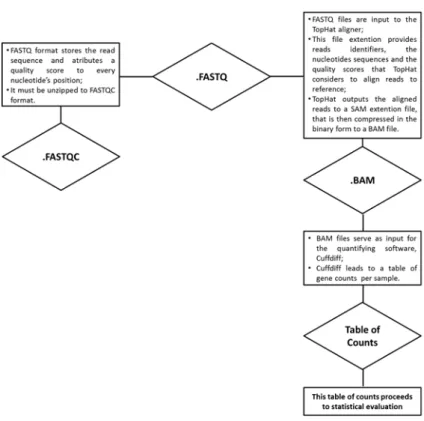
With this in mind, the first step is to assess data quality. This can be done resorting to several tools, such as FastQC, PRINSEQ or FASTX. Focusing on FastQC, this tool reads .fastq files into .fastaqc files. These files are obtained by processing the short reads sequence and attributing a quality score to every base that constitutes it. Hence, these files contain information regarding the read quality. This provides a plateau on the analysis: provided the reads are good the analysis proceeds, if they are not (in other words, if they exhibit unusual qualities, which is a synonym of poor sequencing quality itself, or sequencing contamination), then
2.1. NGS data analysis workflow
Figure 2.2: Different file extensions involved on the NGS data analysis processing.
Chapter 2. Methods for data Analysis
some reparametrization on the NGS technique is required (CBCB, 2013).
The millions of short reads, after quality assessment, will be aligned to a reference resorting to the TopHat mapper. TopHat is based on the short reader aligner Bowtie, and uses it to align reads to a reference. The difference between these two softwares is that TopHat allows gap alignment as well. TopHat will align the reads to the reference using the .fastq files as input (which have the gene coordinates) and return the aligned reads, and the reads that overlap, onto the file extension .sam. These files will be comprised into .bam files, which store the same information but in binary code (CBCB, 2013). The mapping is done with the Borrows-Wheeler algorithm (which is ideal for short reads that have to be aligned to a big reference sequence) and with reads that align only one time, so the obtained reads belong to that gene and that gene only (Oshlack et al. , 2010).
The mapped reads are assembled into an expression summary. For this study, we will consider gene-level counts, which means that the reads are assembled to a gene-level expression summary i.e., the number of reads that fall into a given gene, which is done re-sorting to Cuffdiff. This software receives the .bam files (which are the compressed version of the .sam files) with the aligned reads ob-tained per gene and then counts them, outputting the information on a table of counts that then proceeds to statistical evaluation.
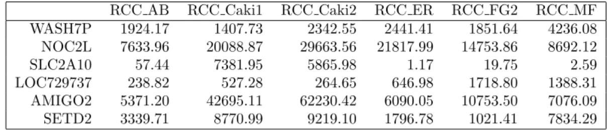
An example of a simple table of counts obtained with this method-ology is as follows in table 2.1, where the g genes are indicated on the rows, and the columns indicate the i samples or libraries. Each cell will correspond to the number of reads aligned to the gene in that sample.
gene mut 1 control 1 control 2 mut 2
1 154 298 120 35 2 16 831 4 273 3 16 155 1 35 4 218 9 63 39 5 982 385 325 163 6 14 5 1 1
Table 2.1: Gene expression matrix example.
When proceeding to the data evaluation, there are two very important steps involved: normalization (chapter 2.2) and differ-ential expression gene analysis (chapter 2.3). These two steps will
2.2. Methods for Normalization
lead to a list of differentially expressed genes, which constitute the biological insight of this project.
2.2
Methods for Normalization
This is the key step leading to the analysis of gene’s Differen-tial Expression, DE. To better understand why, Robinson & Osh-lack (2010) propose a scenario where a large number of genes are uniquely aligned to one of the two experimental conditions in study (in this thesis, mutated or wild type). What happens is that the real sequencing state available for the other genes is shortened. If a large amount of sequencing is dedicated to a specific experimental condition, then there is less sequencing available for the remaining genes. This must be adjusted, otherwise it will lead to a skewed analysis towards one of the experimental conditions (Robinson & Oshlack, 2010),(Oshlack & Wakefield, 2009).
It is therefore imperative to make this data comparable, in a step called normalization. The purpose of this step is to weigh-in systematic technical effects that occur weigh-in the data and remove them, to ensure that systematic bias have minimal impact on the results. A few sources of systematic variation in RNA-seq can be referred. For instance, larger library sizes will typically lead to higher counts for the entire sample, which is described as the overdispersion problem. Another example is that read counts are generally proportional to the gene length. It is important to un-derstand that normalization is necessary in order to only consider sample-specific effects on the analysis, hence removing systematic variations (Robinson et al. , 2010).
During the last 4 years, some normalization approaches on how to treat RNA-seq data have been studied, resulting in several avail-able methodologies, each one considering different assumptions, algorithms, approximations and aspects of the data, to adjust for different bias. But, despite all these studies, there is still not a consensus towards how the choice of normalization influences the downstream analysis (Dillies et al. , 2012).
Bioconductor is an open source software that uses R statistical programming language. This software provides tools for the high-throughput genomic data analysis, conveying numerous software packages designed for the analysis of: DNA microarray, DNA se-quence, a process responsible for genetic variability called Single
Chapter 2. Methods for data Analysis
Nucleotide Polimorfism (SNP) and other data, such as RNA-seq (Bioconductor, 2013). Some of these packages are designed only for data normalization, while some perform both normalization and DE analysis (chapter 2.3).
Considering the methods that have their own protocols for nor-malization and for the identification of differentially expressed genes, DEG, two methods are described in this thesis: edgeR and DESeq (with Bioconductor). Regarding the packages that focuses specifi-cally on normalization, we used the package EDASeq.
2.2.1
edgeR
This package was created in 2008 by Robinson, McCarthy, Chen, Lun and Smyth. Although scaling to library size makes sense, and there are ways to do this (like computing the proportion of every genes reads rendering them to the total number of reads and then comparing it across samples) this might not be enough as a normalization choice. The number of reads that align to a gene is also function of the composition of the RNA population that is being sampled: different experimental conditions express different RNA repertoires and the proportion might not always be directly comparable, which can lead to an over or under sampling effect, misleading DE calls.
With this in mind a new method for normalization was pre-sented by Robinson and Oshlack: the trimmed mean of M-values normalization method, TMM (Robinson & Oshlack, 2010).
Let us consider that the expected value of Ygi is a function of:
the true, yet unknown, expression levels (number of reads), µgi; of
the length of the gene Lg; and of the total RNA output of a sample
Ni, as follows: E[Ygi] = µgiLg Si Ni (2.1) where→Si = G X g=1 µgiLg (2.2)
What equation 2.2 means is that Si is the sum of the number
of reads obtained for every single gene in all libraries, times the length of that library – it represents the total RNA output of a sample, which is unknown and, as mentioned before, can vary a lot according to the RNA population. Si can not be estimated directly
2.2. Methods for Normalization
On the other hand, the relative RNA production of two samples, represented by fi = Si/Si0, can (Robinson & Oshlack, 2010).
Based on this quantity, Robinson and Oshlack assembled a method that equates the overall expression levels of genes between samples, under the premise that most genes are not DE (Oshlack & Wake-field, 2009). What they did was to consider a trimmed mean of the data, where both the log fold-change, log FC, between library i and library r (Mr
gi) and the absolute intensity (Ag) were cut in
order to level the estimates of RNA production, defining them as:
Mgir = log2 Ygi/Ni Ygi0/Ni0 (2.3) Ag = 1 2log2(Ygi/Ni· Ygi0/Ni0) (2.4) The authors then calculated normalization factors by selecting one sample as reference, and calculating TMM factors for the other samples relatively to this reference, so that for every tested sample, TMM is computed as the weighted mean of log ratios between the test and the reference sample, excluding the most expressed genes and the genes with the highest log ratios. Given the hypothesis that the majority of genes are not DE – the null hypothesis – this TMM should be close to one. If it is not, then the value obtained provides the correction factor to be applied to the library sizes in order to be in agreement with H0. In R, the function calcNormFactors()
calculates these normalization factors. To obtain the normalized read counts, the software must consider these normalization factors and re-scale them by the mean of the normalized library sizes. The normalized read counts per se are retrieved by dividing the raw read counts by these re-scaled normalization factors (Dillies et al. , 2012). This method provides a robust way to weight in relative RNA production levels, with the normalization factors proceeding directly to DE analysis.
2.2.2
DESeq
DESeq was developed by Anders and Huber (2010). DESeq and edgeR both base their normalization method on the hypothesis that most genes are not DE, although they adopt different approaches. Being that said, Anders and Huber (Anders & Huber, 2010) developed a method of normalization where, along with Ygi, they introduce,
Chapter 2. Methods for data Analysis
si, the size factor which stands for the effective size of library i.
In the normalization step, m size factors, si, are estimated from
the count data, resorting to the median of the ratios of observed counts for all genes, as follows:
b si = mediani kgi (Qm υ=1kgυ)1/m (2.5) The denominator of equation 2.5 is interpreted as a reference sample, to which every size factor is compared (Anders & Huber, 2012).
The authors created a method that, like edgeR, takes into ac-count that the total number of reads might not be a factor good enough to normalize the data. They admit that there might be some highly differentially expressed genes that can have a big in-fluence on the total read counts, and this will lead to a biased DE analysis, if not normalized. They then devised a method where each sample – column – is divided by the geometric mean of the rows – genes – and the median of these ratios is the sizing factor for the sample in question (Rapaport et al. , 2013).
In R the normalization is reached with the functions estimateSizeFactors() and sizeFactors(), where the size factors are computed for each sample, and the counts are divided by the factor associated with that sample (Anders, 2010).
2.2.3
EDASeq
Thus far, it has been stated in this chapter, how some fragments characteristics make them preferentially detected with RNA Seq techniques (Hansen et al. , 2012). An example that has already been stated, is that longer genes tend to bias the analysis, as they typically tend to have more reads aligned to them. An-other strong example is the effect of GC content, which has been shown to affect DNA related measurements, such as RNA Seq (Pickrell et al. , 2010). Pickrell et al have demonstrated GC-content effect can change from sample to sample and Benjamini & Speed (2007) have demonstrated that both genes with high content GC and low content GC reveal this sample specific effect (Ben-jamini & Speed, 2012).
With this knowledge regarding GC-content effect, Risso and Dudoit created EDASeq package, 2010. These authors took a differ-ent approach from the two methods described before: they
con-2.2. Methods for Normalization
sider that there are two types of effects on read counts, within-lane gene-specific effects and between-within-lane distributional differ-ences effects. These two types of effects lead to a two step nor-malization process: within lane normalization accounts for GC content or gene length biases, while between lane normalization focuses on normalization for the sequencing depth (Risso, 2011). In essence, the approach this authors made is different from edgeR and DESeq, because the EDASeq package has this dual approach, by first considering a lane-specific normalization – GC content or gene length (within normalization) – and only then accounting for the sequencing depth (between normalization)(Bullard et al. , 2010). The normalization is achieved with withinLaneNormalization() and betweenLaneNormalization() functions.
The authors consider several options for either within and be-tween normalization. Within-lane normalization has four approaches to adjust for GC content or to gene length effect on the sample: loess robust local regression, global-scaling, using the median or the upper quantile, and full-quantile normalization. Loess regres-sion will perform a regresregres-sion on the data, according to the gene effect of interest (either GC content or gene length) (Risso et al. , 2011). The three approaches that use quantiles will be function of a defined number of equally sized bins. These bins divide the data according to GC content in several stratus: global scaling using the median will scale the data to have the same median for each bin, global scaling using the upper quantile scales the data to have the same upper quantile and full-quantile normalization will take the several bins quantiles and pair them in order to obtain the me-dian for every quantile. This is an approach similar to microarrays where, for each lane, the distribution of read counts is matched to a reference distribution, that is defined according to the median counts of the sorted lane (Bullard et al. , 2010).
Between-lane normalization adjusts for lane sequencing depth, i.e., by the number of total read counts per lane i. This nor-malization aims at rendering lane differences, making the samples comparable. The authors postulated three different types of malization procedures, the same above referred: global-scaling nor-malization using upper quantile, global-scaling nornor-malization using the median and full quantile normalization. The way these normal-izations process the quantiles is the same as described for within normalization but applied to the lanes in study. Hence, global scal-ing usscal-ing the median will force the median of each lane to be the
Chapter 2. Methods for data Analysis
same, global scaling using the upper quantile will force the upper quantile of each lane to be the same and full quantile normalization will take the quantiles of each lane and pair the median of every quantile (Bullard et al. , 2010).
This package focuses specifically in data normalization, creat-ing an EDASeq object of normalized data count, to be used for DE analysis by DESeq and edgeR.
2.3
Methods for Differential Expression Gene
analysis
The previous normalization step will lead to normalized count data, on the form of a matrix, where each cell will correspond to the number of reads aligned to gene g in sample i. This count data matrix will constitute the input for a differential expression gene analysis. DE analysis is used to measure differences in expression levels between two conditions, allowing the analyst to infer about the genomic structure under study, either a known sequence, or a de novo sequencing.
As normalization takes into account different considerations that lead to different normalized count data, DE analysis also has meth-ods based on distinct premises, that lead to alternative ways to achieve differential expression.
Being that said, different statistical methods can be assumed for DE analysis. The selected methods to be presented in this thesis are: edgeR, DESeq and RankProd. RankProd has the characteristics of not only considering a non-parametric approach – while all others assume parametric assumptions – but also being meant for mi-croarray analysis. Other methods examples are NOISeq, DEXseq, DEGseq, which were not considered in our analysis, since these are not as used in the literature.
The considered methods are all based on the null hypothesis that genes are not differentially expressed against the alternative hypothesis that they are differentially expressed. The five meth-ods provide statistical elements that allow the user to infer about differential expression analysis and gene regulation. To be men-tioned, and of key importance, are the log fold-change, log FC, and the false discovery rate, FDR (Benjamini & Hochberg, 1995). The log fold-change calculation, logFC, is computed between
2.3. Methods for Differential Expression Gene analysis
two experimental conditions. It is calculated by dividing two val-ues, A and B, that reflect gene expression measured under two different experimental conditions, typically between mutated and control (Robinson et al. , 2010).
FDR is a measure used in multiple testing: it controls the num-ber of false discoveries in tests that result in a positive result (i.e. significant result). Multiple testing corrections will adjust p-values derived from multiple statistical tests, in order to correct for oc-currence of false positives. This is better explained resorting to an example: a p-value of 0.05 would imply that 5% of all tests result in false positives. However, when considering an adjusted p-value of 0.05, what is being considered is that that 5% of significant tests will result in false positives. Methods for multiple testing whose aim is to decrease FDR (like Benfamini-Hochberg) imply smaller adjusted p-values (Benjamini & Hochberg, 1995). This is a mea-sure typically used in microarrays or NGS data, given the amount of tests performed in such gene-expression analysis.
2.3.1
edgeR
In order to perform statistical testing, edgeR fits the data to a nega-tive binomial distribution, NB. NB distribution has different mean and variance. This gives more reliability than the Poisson distribu-tion (which is by definidistribu-tion the model used for count data), given this distribution assumes the same value for the mean and the vari-ance – unlike Poisson, over dispersion is accounted for within NB distribution (Robinson & Smyth, 2007). This being said, the NB distribution allows the possibility of gene-specific variability (some genes may show different biological variability from one another) and this is accounted for.
The gene counts are thus modelled as follows:
Ygij ∼ NB(Mipgj; φg) (2.6)
with E(Ygij) = µij = Mipgj (2.7)
and var(Ygij) = µij(1 + µijφg) (2.8)
with Ygij being the number of counts for gene g in library i and
replicate j, Mi the library size for library i, pgi the proportion of
reads for gene g in library i and φg the overdisperson parameter
Chapter 2. Methods for data Analysis
edgeR devises two levels of variation: biological and technical variation. The package considers the dispersion parameter, φg, as
the square of the coefficient of variation, CV (φg = CV2). CV is
given, by definition, by the sum of the square of the biological co-efficient of variation, BCV and the square of the technical CV, as follows (with BCV being the dominant source of variation) (Mc-Carthy et al. , 2012):
CV2 = BCV2+ T echnicalCV2 (2.9) The first step towards differential expression gene analysis is to model the data dispersion parameter, which determines how to model the variance for each gene. This is done by first es-timating the common dispersion parameter for the genes, with estimateCommonDisp() function. With this consideration, all the genes are admitted to have the same value for dispersion when modelling the variance. The authors assume an extension to this tactics, given by estimateTagwiseDisp() function, where genes as-sume their own dispersion value, while also rendering it to the common dispersion estimate obtained with estimateCommonDisp() function. This adjustment is done with a quantile adjusted con-ditional maximum likelihood test, qCML, which searches for an equilibrium between common and tagwise dispersion (Robinson & Smyth, 2008).
The method these authors built introduces this weighted condi-tional likelihood estimator that considers tagwise dispersion when estimating the common dispersion. This shrinkage considers an approximate empirical Bayes rule, which adapts the similarity of the dispersions, considering sample sizes, scores and informations (Robinson & Smyth, 2007).
To test the difference between expression levels under two con-ditions, these authors use an exact test, analogous to Fisher?s exact test or the likelihood ratio test, LRT. For both, the quantile ad-justment considered for qCML is used to adjust the tag counts to a common library size (Robinson & Smyth, 2007). The exact test was developed for experimental data with single factor, while LRT, which is in fact a LRT test for a Generalized Linear Model, GLM, was design mainly for experiments with multiple factor de-sign. However, this is outside the context of this project, where we worked with single factor design experiment.
2.3. Methods for Differential Expression Gene analysis
2.3.2
DESeq
As in edgeR, DESeq package also assumes data to follow a NB distri-bution, thus addressesing this “over dispersion” problem by mod-elling the number of read counts for gene g in sample i (Ygi)
re-sorting to the Negative Binomial distribution, whose parameters are determined by µgi (mean) and σgi2 (variance) (Anders & Huber,
2012).
Ygi ∼ NB(µgi; σ2gi) (2.10)
The mean is expressed as the product of qg,ρ(i), and si, as follows:
µgi= qg,ρ(i)si (2.11)
where ρ(i) is the experimental condition of sample i and qg,ρ(i) is
therefore a condition value for a given experimental condition on a specific sample i on gene g ; qg,ρ(i) is proportional to the expected
value of the true (but unknown) concentration of fragments from gene g, under condition i ; si is the size factor for sample i. This is
particularly important when estimating the library size.
The variance: σ2gi, reflects the dispersions to each gene, it is the sum of the shot noise and the raw variance.
σ2gi= µgi+ s2iυg,ρ(i) (2.12)
The shot noise, µgi, is the name given to the uncertainty in
measuring a concentration by counting reads. It is dominating in lowly expressed genes. The raw variance, s2
iυg,ρ(i), is the
sample-to-sample variation, this term traduces the effective variance in the counts and it is dominating in highly expressed genes (Anders & Huber, 2010). The shot noise is a function of qg and ρ(i):
υg,ρ(i)= υρ(qg,ρ(i)) (2.13)
When fitting the model, the first step is to define a table of counts of sequencing reads. These counts cannot be rounded, nor can they be counts of covered based pairs, DESeq is designed to work with raw counts.
Then, the package must be provided with a data.frame that stores information about the samples and their features, each row being a sample and each column being a feature about the sample, such as type of library or sample conditions. It can store size sam-ple annotations, conditions and size factors – this is called metadata (Anders, 2010).