Search for doubly charged Higgs boson production in multi-lepton final states with the ATLAS detector using proton–proton collisions at $\sqrt{s}=13\,\text {TeV}$

EUROPEAN ORGANISATION FOR NUCLEAR RESEARCH (CERN)

Eur. Phys. J. C78 (2018) 199

DOI:10.1140/EPJC/S10052-018-5661-Z

CERN-EP-2017-198 19th March 2018

Search for doubly charged Higgs boson

production in multi-lepton final states with the

ATLAS detector using proton–proton collisions at

_√

s

= 13 TeV

The ATLAS Collaboration

A search for doubly charged Higgs bosons with pairs of prompt, isolated, highly energetic leptons with the same electric charge is presented. The search uses a proton–proton collision

data sample at a centre-of-mass energy of 13 TeV corresponding to 36.1 fb−1of integrated

luminosity recorded in 2015 and 2016 by the ATLAS detector at the LHC. This analysis focuses on the decays H±± → e±e±, H±±→ e±µ±and H±±→µ±µ±, fitting the dilepton mass spectra in several exclusive signal regions. No significant evidence of a signal is observed and corresponding limits on the production cross-section and consequently a lower limit on m(H±±) are derived at 95% confidence level. With `±`± = e±e±/µ±µ±/e±µ±, the observed lower limit on the mass of a doubly charged Higgs boson only coupling to left-handed leptons

varies from 770 GeV to 870 GeV (850 GeV expected) for B(H±± →`±`±)= 100% and both

the expected and observed mass limits are above 450 GeV for B(H±± → `±`±) = 10% and

any combination of partial branching ratios.

c

2018 CERN for the benefit of the ATLAS Collaboration.

1 Introduction

Events with two prompt, isolated, highly energetic leptons with the same electric charge (same-charge leptons) are produced very rarely in a proton–proton collision according to the predictions of the Standard Model (SM), but may occur with higher rate in various theories Beyond the Standard Model

(BSM). This analysis focuses on BSM theories that contain a doubly charged Higgs particle H±±using

the observed invariant mass of same-charge lepton pairs. In the absence of evidence for a signal, lower limits on the mass of the H±±particle are set at the 95% confidence level.

Doubly charged Higgs bosons can arise in a large variety of BSM theories, namely in left-right sym-metric (LRS) models [1–5], Higgs triplet models [6, 7], the little Higgs model [8], type-II see-saw models [9–13], the Georgi–Machacek model [14], scalar singlet dark matter [15], and the Zee–Babu neutrino mass model [16–18]. Theoretical studies [19–21] indicate that the doubly charged Higgs bosons would be predominantly pair-produced via the Drell–Yan process at the LHC. For this search, the cross-sections utilised to set the final exclusion limits are computed according to the model in Ref. [9].

Doubly charged Higgs particles can couple to either left-handed or right-handed leptons. In LRS mod-els, two cases are distinguished and denoted H±±_L and H±±_R . The cross-section for H_L++H−−_L production is about 2.3 times larger than for H_R++H_R−−due to the different couplings to the Z boson [22]. Besides

the leptonic decay, the H±± particle can decay into a pair of W bosons as well. For low values of

the Higgs triplet vacuum expectation value v_∆, it decays almost exclusively to leptons while for high values of v_∆the decay is mostly to a pair of W bosons [9, 12]. In this analysis, the coupling to W bosons is assumed to be negligible and only pair production via the Drell–Yan process is considered.

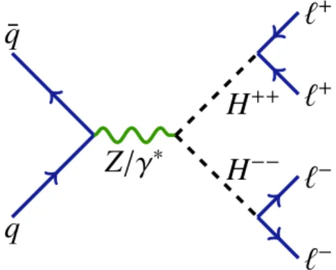
The Feynman diagram of the production mechanism is presented in Figure1.

The analysis targets only decays of the H±± particle into electrons and muons, denoted by `. Other

final states X that are not directly selected in this analysis are taken into account by reducing the lepton multiplicity of the final state. These states X would include, for instance, τ leptons or W

bosons, as well as particles which escape detection. The total assumed branching ratio of H±± is

therefore B(H±± → e±e±)+ B(H±± → e±µ±)+ B(H±± → µ±µ±)+ B(H±± → X) = B(H±± →

`±<sub>`</sub>±_{)+ B(H}±± _{→ X)= 100%. Moreover, the decay width is assumed to be negligible compared to}

the detector resolution, which is compatible with theoretical predictions. Two-, three-, and four-lepton signal regions are defined to select the majority of such events. These regions are further divided into unique flavour categories (e or µ) to increase the sensitivity. The partial decay width of H±±to leptons is given by: Γ(H±± →`±`0±)= kh 2 ``0 16πm(H ±± ),

with k = 2 if both leptons have the same flavour (` = `0) and k = 1 for different flavours. The

factor h``0has an upper bound that depends on the flavour combination [23,24]. In this analysis, only prompt decays of the H±±bosons (cτ < 10 µm) are considered, corresponding to h``0 & 1.5 × 10−6for m(H±±)= 200 GeV. In general, there is no preference for decays into τ leptons, as the coupling is not proportional to the lepton mass like it is for the SM Higgs boson.

¯q

q

Z/γ

H

H

`

`

`

`

Figure 1: Feynman diagram of the pair production process pp → H++H−−. The analysis studies only the

electron and muon channels, where at least one of the lepton pairs is e±e±, e±µ±, or µ±µ±.

Additional motivation to study cases with B(H±± →`±`±) < 100% is given by type-II see-saw models with specific neutrino mass hypotheses resulting in a fixed branching ratio combination [13,25,26]

which does not necessarily correspond to B(H±±→`±`±)= 100%.

The ATLAS Collaboration previously analysed data corresponding to 20.3 fb−1of integrated

lumin-osity which were recorded in 2012 at a centre-of-mass energy of 8 TeV [27]. This study resulted

in the most stringent lower limits on the mass of a potential H±±_L particle. Depending on the

fla-vour of the final-state leptons, the observed limits vary between 465 GeV and 550 GeV assuming B(H±±_L →`±`±) = 100%. The analysis presented in this paper extends the one described in Ref. [27]

and is based on 36.1 fb−1 of integrated luminosity collected in 2015 and 2016 at a centre-of-mass

energy of 13 TeV. A similar search has also been performed by the CMS Collaboration [28].

2 ATLAS detector

The ATLAS detector [29] at the LHC is a multi-purpose particle detector with a forward-backward

symmetric cylindrical geometry and an almost 4π coverage in solid angle.1 It consists of an inner

tracking detector (ID) surrounded by a thin superconducting solenoid providing a 2 T axial magnetic field, electromagnetic (EM) and hadronic calorimeters, and a muon spectrometer. The inner tracking detector covers the pseudorapidity range |η| < 2.5. It is composed of silicon pixel, silicon micro-strip, and transition radiation tracking detectors. A new innermost layer of pixel detectors [30] was installed prior to the start of data taking in 2015. Lead/liquid-argon (LAr) sampling calorimeters

provide electromagnetic energy measurements with high granularity. A hadronic (steel

/scintillator-tile) calorimeter covers the central pseudorapidity range (|η| < 1.7). The end-cap and forward re-gions are instrumented with LAr calorimeters for both EM and hadronic energy measurements up to |η| = 4.9. The muon spectrometer surrounds the calorimeters and features three large air-core toroidal superconducting magnets with eight coils each. The field integral of the toroids ranges between 2.0 to

1_{ATLAS uses a right-handed coordinate system with its origin at the nominal interaction point (IP) in the centre of the}

detector and the z-axis along the beam pipe. The x-axis points from the IP to the centre of the LHC ring, and the y-axis points upwards. Cylindrical coordinates (r, φ) are used in the transverse plane, φ being the azimuthal angle around the

z-axis. The pseudorapidity is defined in terms of the polar angle θ as η= − ln tan(θ/2). Angular distance is measured in

units of∆R ≡ p(∆η)2+ (∆φ)2_{. Rapidity is defined as y ≡ 0.5 ln [(E}+ p

z)/(E − pz)] where E denotes the energy and pz

6.0 T m across most of the detector. The muon system includes precision tracking chambers and fast detectors for triggering. A two-level trigger system is used to select events [31] that are interesting for physics analyses. The first-level trigger is implemented as part of the hardware. Subsequently a software-based high-level trigger executes algorithms similar to those used in the offline reconstruc-tion software, reducing the event rate to about 1 kHz.

3 Dataset and simulated event samples

The data used in this analysis were collected at centre-of-mass energy of 13 TeV during 2015 and

2016, and correspond to an integrated luminosity of 3.2 fb−1 in 2015 and 32.9 fb−1 in 2016. The

average number of pp interactions per bunch crossing in the dataset is 24. Interactions other than the hard-scattering one are referred to as pile-up. The uncertainty on the combined 2015 and 2016

integrated luminosity is 3.2%. Following a methodology similar to the one described in Ref. [32],

this uncertainty is derived from a preliminary calibration of the luminosity scale using x–y beam-separation scans performed in August 2015 and May 2016.

Signal candidate events in the electron channel are required to pass a dielectron trigger with a threshold

of 17 GeV on the transverse energy (ET) of each of the electrons. Candidate events in the muon

chan-nel are selected using a combination of two single-muon triggers with transverse momentum (pT)

thresholds of 26 GeV and 50 GeV. The single-muon trigger with the lower pT threshold also

re-quires track-based isolation of the muon according to the isolation criteria described in Ref. [33].

Events containing both electrons and muons (mixed channel) are required to pass either the combined electron–muon trigger or any of the triggers used for the muon channel or the electron channel. The

combined trigger has an ET threshold of 17 GeV for the electron and a pT threshold of 14 GeV for

the muon. Events with four leptons are selected using a combination of dilepton triggers. In gen-eral, single-lepton triggers are more efficient than dilepton triggers. However, single-electron triggers impose stringent electron identification criteria, which interfere with the data-driven background es-timation.

An irreducible background originates from SM processes resulting in same-charge leptons, hereafter referred to as prompt background. Prompt background and signal model predictions were obtained

from Monte Carlo (MC) simulated event samples which are summarised in Table 1. Prompt

back-ground events mainly originate from diboson (W±W± / ZZ / WZ) and t¯tX processes (t¯tW, t¯tZ, and

t¯tH). They also provide a source of reducible background due to charge misidentification in channels that contain electrons.2 As described in Section5, the modelling of charge misidentification in simu-lation deviates from data and consequently charge reconstruction scale factors are derived in a data-driven way and applied to the simulated events to compensate for the differences. The highest-yield process which enters the analysis through charge misidentification is Drell–Yan (q ¯q → Z/γ∗→`+`−) followed by t¯t production. MC samples are in general normalised using theoretical cross-sections

referenced in Table1. However, yields of some MC samples are considered as free parameters in the

likelihood fit, as described in Section7.

Another source of reducible background arises from events with non-prompt electrons or muons or with other physics objects misidentified as electrons or muons, collectively called ‘fakes’. For both,

2_{The probability of muon charge misidentification is negligible because muon tracks are measured both in the inner}

Table 1: Simulated signal and background event samples: the corresponding event generator, parton shower, cross-section normalisation, PDF set used for the matrix element and set of tuned parameters are shown for each sample. The cross-section in the event generator that produces the sample is used where not specifically stated otherwise.

Physics process Event generator ME PDF set Cross-section Parton shower Parton shower

normalisation tune

Signal

H±± Pythia 8.186 [34] NNPDF2.3NLO [35] NLO (see Table2) Pythia 8.186 A14 [36] Drell–Yan

Z/γ∗_{→ ee/ττ Powheg-Box v2 [37–39] CT10 [40] NNLO [41] Pythia 8.186 AZNLO [42]} Top

t¯t Powheg-Box v2 NNPDF3.0NLO [43] NNLO [44] Pythia 8.186 A14

Single top Powheg-Box v2 CT10 NLO [45] Pythia 6.428 [46] Perugia 2012 [47] t¯tW, t¯tZ/γ∗ _{MG5_aMC@NLO 2.2.2 [48] NNPDF2.3NLO NLO [49] Pythia 8.186 A14}

t¯tH MG5_aMC@NLO 2.3.2 NNPDF2.3NLO NLO [49] Pythia 8.186 A14

Diboson

ZZ, WZ Sherpa 2.2.1 [50] NNPDF3.0NLO NLO Sherpa Sherpa default

Other (inc. W±_W±_{) Sherpa 2.1.1 CT10 NLO Sherpa Sherpa default}

Diboson Sys.

ZZ, WZ Powheg-Box v2 CT10NLO NLO Pythia 8.186 AZNLO

electrons and muons, this contribution originates within jets, from decays of light-flavour or heavy-flavour hadrons into light leptons. For electrons, a significant component of fakes arises from jets which satisfy the electron reconstruction criteria and from photon conversions. MC samples are not used to estimate this background because the simulation of jets and hadronisation has large uncertain-ties. Instead, a data-driven approach is used to assess this contribution from production of W+jets, t¯t and multi-jet events. The method is validated in specialised validation regions.

The SM Drell–Yan process was modelled using Powheg-Box v2 [37–39] interfaced to Pythia 8.186 [34]

for parton showering. The CT10 set of parton distribution functions (PDF) [40] was used to

calcu-late the hard scattering process. A set of tuned parameters called the AZNLO tune [42] was used in

combination with the CTEQ6L1 PDF set [51] to model non-perturbative effects. Photos++ version

3.52 [52] was used for photon emissions from electroweak vertices and charged leptons. The

genera-tion of the process was divided into 19 samples with subsequent invariant mass intervals to guarantee a good statistical coverage over the entire mass range.

Higher-order corrections were applied to the Drell–Yan simulated events to scale the mass-dependent cross-section computed at next-to-leading order (NLO) in the strong coupling constant with the CT10 PDF set to next-to-next-to-leading order (NNLO) in the strong coupling constant with the CT14NNLO PDF set [41]. The corrections were calculated with VRAP [53] for QCD effects and Mcsanc [54] for electroweak effects. The latter are corrected from leading-order (LO) to NLO.

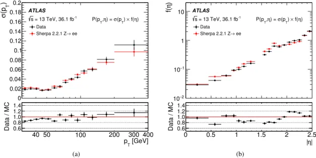
A sample of Z → ee events was generated with Sherpa 2.2.1 [50], in addition to the Powheg prediction, to measure the probability of electron charge misidentification, as explained in Section5. The electron

pT spectrum is a crucial ingredient for the estimate of this probability and was found to be better

described by Sherpa than by Powheg, especially for invariant masses of the electron pair close to the

Z_{boson mass. Sherpa uses Comix [}55] and OpenLoops [56] to calculate the matrix elements up to

two partons at NLO and up to four partons at LO in the strong coupling constant. The merging with

The t¯t process was generated with the NLO QCD event generator Powheg-Box v2 which was

inter-faced to Pythia 8.186 for parton showering. The A14 parameter set [36] was used together with the

NNPDF2.3 [35] PDF set for tuning the shower. Furthermore, the PDF set used for generation was

NNPDF3.0 [43]. Additionally, top-quark spin correlations were preserved through the use of

Mad-Spin [59]. The predicted t¯t production cross-section is 832+20₋₃₀(scale) ±35 (PDF+ αS) pb as calculated

with Top++2.0 [44] to NNLO in perturbative QCD, including soft-gluon resummation to

next-to-next-to-leading-log order. The top-quark mass was assumed to be 172.5 GeV. The scale uncertainty results from independent variations of the factorisation and renormalisation scales, while the second

uncer-tainty is associated with variations of the PDF set and αS, following the PDF4LHC[60] prescription

using the MSTW2008 68% CL NNLO[61], CT10 NNLO [62], and NNPDF2.3 PDF sets.

Single-top-quark events produced in Wt final states were generated by Powheg-Box v2 with the CT10 PDF set used in the matrix element calculations. Single-top-quark events in other final states were generated by Powheg-Box v1. This event generator uses the four-flavour scheme for the NLO QCD matrix element calculations together with the fixed four-flavour PDF set CT10f4. The parton shower,

hadronisation, and underlying event were simulated with Pythia 6.428 [46] using the CTEQ6L1 PDF

set and the corresponding Perugia 2012 tune (P2012) [47]. The top-quark mass was set to 172.5 GeV.

The NLO cross-sections used to normalise these MC samples are summarised in Ref. [45].

The t¯tW, t¯tZ, and t¯tH processes were generated at LO with MadGraph v2.2.2 [63] and

Mad-Graph v2.3.2 using the NNPDF2.3 PDF set. Pythia 8.186 was applied for shower modelling con-figured with the A14 tune [36], as explained in more detail in Ref. [64]. They were normalised using theoretical cross-sections summarised in Ref. [49].

Diboson processes with four charged leptons, three charged leptons and one neutrino, or two charged leptons and two neutrinos were generated with Sherpa 2.2.1, using matrix elements containing all diagrams with four electroweak vertices. They were calculated for up to three partons at LO ac-curacy and up to one (4`, 2`+2ν) or zero partons (3`+1ν) at NLO QCD using Comix and

Open-Loops. The merging with the Sherpa parton shower [57] follows the ME+PS@NLO prescription.

The NNPDF3.0NNLO [43] PDF set was used in conjunction with dedicated parton shower tuning by

the Sherpa authors.

Diboson processes with one boson decaying hadronically and the other one decaying leptonically were predicted by Sherpa 2.1.1 [50]. They were calculated for up to three additional partons at LO accuracy and up to one (ZZ) or zero (WW, WZ) additional partons at NLO using Comix and OpenLoops matrix

element generators. The merging with the Sherpa parton shower [57] follows the ME+PS@NLO

prescription. The CT10 PDF set was used in conjunction with a dedicated parton shower tuning. The Sherpa 2.1.1 diboson prediction was scaled by 0.91 to account for differences between the internal

electroweak scheme used in this Sherpa version and the Gµ scheme which is the common default.

Similarly, loop-induced diboson production with both gauge bosons decaying fully leptonically was simulated with Sherpa 2.1.1. The prediction is at LO accuracy while up to one additional jet is merged with the matrix element.

Additional diboson samples for WZ and ZZ production were generated with Powheg-Box v2 to estim-ate theoretical uncertainties. Pythia 8.186 provided the parton shower. The CT10 PDF set was used for the matrix element calculation while the parton shower was configured with the CTEQL1 PDF set.

The non-perturbative effects were modelled using the AZNLO [42] tune.

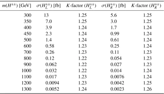
Signal samples were generated at LO using the LRS package of Pythia 8.186 which implements the

Table 2: NLO cross-sections for the pair production of H_L++H−− L and H++R H −− R in pp collisions at √ s= 13 TeV,

together with the correction factors (K= σNLO/σLO) used to obtain those values from the LO prediction. These

K-factors are calculated by the authors of Ref. [9] using the CTEQ6 PDF [65].

m(H±±) [GeV] σ(H±±_L ) [fb] K-factor (H_L±±) σ(H_R±±) [fb] K-factor (H±±_R )

300 13 1.25 5.6 1.25 350 7.0 1.25 3.0 1.25 400 3.9 1.24 1.7 1.24 450 2.3 1.24 0.99 1.24 500 1.4 1.24 0.61 1.24 600 0.58 1.23 0.25 1.24 700 0.26 1.23 0.11 1.23 800 0.12 1.22 0.054 1.23 900 0.062 1.22 0.027 1.23 1000 0.032 1.22 0.014 1.24 1100 0.017 1.23 0.0076 1.24 1200 0.0094 1.23 0.0042 1.25 1300 0.0052 1.24 0.0023 1.26

The h``0couplings of lepton pairs were assumed to be the same for H±±

R and H

±±

L particles. This choice

resulted in a good statistical coverage for all possible decay channels. The production of the H±±was

implemented only via the Drell–Yan process. Originally, the cross-section at √s = 14 TeV was

calculated with NLO accuracy by the authors of Ref. [9]. Subsequently, a rescaling to √s = 13 TeV

with the CTEQ6 PDF [65] set was provided. The cross-sections and corresponding K-factors are

summarised in Table2.

Since this analysis exclusively targets the leptonic decays of the H±±bosons, the vacuum expectation

value of the neutral component of the left-handed Higgs triplet (vL_∆) was set to zero in order to exclude

H±± → WW decays. The decay width of the H±± particle to leptons depends on the h``0 couplings.

These were set to the value h``0 = 0.02 in all Pythia 8.186 samples. This setting corresponds to a

decay width that is negligible compared to the detector resolution. The h`τ and hττ couplings were

fixed at zero. There are 23 MC samples with different H±± particle masses, starting from 200 GeV

up to 1300 GeV in steps of 50 GeV. The ATLAS detector is expected to have the best H±± mass

resolution in the electron–electron final states. Resolutions around 30 GeV for masses of 200-500 GeV and 50 GeV to 100 GeV for higher masses can be achieved with the event selection defined in Section4.

Furthermore, the H±± mass resolution in electron–muon final states varies from 50 GeV to 150 GeV

and from 50 GeV to 200 GeV in muon–muon final states.

For all simulated samples except those obtained with Sherpa, the EvtGen v1.2.0 program [66] was

used to model bottom and charm hadron decays. The effect of the pile-up was included by overlay-ing minimum-bias collisions, simulated with Pythia 8.186, on each generated signal and background event. The number of overlaid collisions is such that the distribution of the average number of inter-actions per pp bunch crossing in the simulation matches the pile-up conditions observed in the data. The pile-up simulation is described in more detail in Ref. [67].

The response of the ATLAS detector was simulated using the Geant 4 toolkit [68]. Data and

simu-lated events were reconstructed with the default ATLAS software [69] while simulated events were

corrected with calibration factors to better match the performance measured in data.

4 Event reconstruction and selection

Events are required to have at least one reconstructed primary vertex with at least two associated

tracks with pT > 400 MeV. Among all the vertices in the event the one with the highest sum of

squared transverse momenta of the associated tracks is chosen as the primary vertex.

4.1 Event reconstruction

This analysis classifies leptons in two exclusive categories called tight and loose, defined specifically for each lepton flavour as described below. Leptons selected in the tight category feature a predom-inant component of prompt leptons, while loose leptons are mostly fakes, which are used for the fake-background estimation. All tracks associated with lepton candidates must have a longitudinal impact parameter with respect to the primary vertex of less than 0.5 mm.

Electron candidates are reconstructed using information from the EM calorimeter and ID by match-ing an isolated calorimeter energy deposit to an ID track. They are required to have |η| < 2.47, pT > 30 GeV, and to pass at least the LHLoose identification level based on a multivariate likelihood discriminant [70,71]. The likelihood discriminant is based on track and calorimeter cluster informa-tion. Electron candidates within the transition region between the barrel and endcap electromagnetic calorimeters (1.37 < |η| < 1.52) are vetoed due to limitations in their reconstruction quality. The track associated with the electron candidate must have an impact parameter evaluated at the point of closest approach between the track and the beam axis in the transverse plane (d0) that satisfies |d0|/σ(d0) < 5, where σ(d0) is the uncertainty on d0. In addition to this, electron candidates are classified as tight if they satisfy the LHMedium working point of the likelihood discriminant and the isolation criteria described in Ref. [70]. This is based on calorimeter cluster and track isolation, which vary to obtain

a fixed efficiency for selecting prompt electrons of 99% across pT and η. Electrons are classified as

loose if they fail to satisfy either of the identification or the isolation criteria.

Muon candidates are selected by combining information from the muon spectrometer and the ID. They satisfy the medium quality criteria described in Ref. [33] and are required to have pT > 30 GeV, |η| < 2.5 and |d0|/σ(d0) < 10. Muon candidates are classified as tight if their impact parameter satisfies |d0|/σ(d0) < 3.0 and they satisfy the most stringent isolation working point of the cut-based track isolation [70]. Muons are loose if they fail the isolation requirement.

Jets or particles originating from the hadronisation of partons are reconstructed by clustering energy deposits in the calorimeter calibrated at the EM scale. The anti-ktalgorithm [72] is used with a radius

parameter of 0.4, which is implemented with the FastJet [73] package. The majority of pile-up jets

are rejected using the jet-vertex-tagger [74], which is a combination of track-based variables provid-ing discrimination against pile-up jets. For all jets the expected average transverse energy contribution from pile-up is subtracted using an area-based pTdensity subtraction method and a residual correction derived from the MC simulation, both detailed in Refs. [75, 76]. In this analysis, events containing

jets identified as originating from b-quarks are vetoed. They are identified with a multivariate dis-criminant [76] that has a b-jet efficiency of 77% in simulated t¯t events and a rejection factor of ≈ 40 (≈ 20) for jets originating from gluons and light quarks (c-quarks).

After electron and muon identification, jet calibration, and pile-up jet removal, overlaps between reconstructed particles or jets are resolved. First, electrons are removed if they share a track with a muon. Secondly, ambiguities between electrons and jets are resolved. If a jet is closer than p

(∆y)2+ (∆φ)2 = 0.2 the jet is rejected. If 0.2 < p(∆y)2+ (∆φ)2 < 0.4 the electron is removed.

Finally, if a muon and a jet are closer than p(∆y)2+ (∆φ)2 = 0.4, and the jet features less than 3

tracks, the jet is removed. Otherwise the muon is discarded.

4.2 Event selection

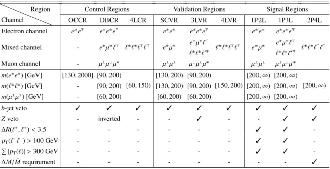
In this search, events are classified in independent categories, called analysis regions, which serve different purposes. The so-called control regions are used to constrain free background parameters

in the statistical analysis detailed in Section 7. The background model is validated against data in

validation regions. Both the control and validation regions are designed to reject signal events. A dedicated selection targeting signal events is utilised to define the signal regions. The selection criteria utilised for each region are summarised in Table3. The main variable that defines the type of the region is the invariant mass of same-charge lepton pairs. Invariant masses are required to be above 200 GeV in signal regions and below 200 GeV in most control and validation regions.

The lepton multiplicity in the event is used to define the analysis regions. Events with two or three leptons are required to contain exactly one same-charge lepton pair, while four-lepton events are required to feature two same-charge pairs where the sum of all lepton charges has to be zero. An exception is the opposite-charge control region (OCCR) where exactly two electrons with opposite charge are required. In all regions, events with at least one b-tagged jet are vetoed, in order to suppress background events arising from top-quark decays. In regions with more than two leptons, events are rejected if any opposite-charge same-flavour lepton pair is within 10 GeV of the Z boson mass (81.2 GeV < m(`+`−) < 101.2 GeV). This requirement is applied to reject diboson events featuring a Z boson in the final state, and is inverted in diboson control regions, where at least one Z boson is present. Furthermore, the Z boson veto is not applied in four-lepton control and validation regions to increase the available number of simulated diboson events.

The invariant mass of the same-charge lepton pair is used in the final fit of the analysis for the two-and three-lepton regions. In the OCCR, the invariant mass of the opposite-charge lepton pair is used. A lower bound of 60 GeV on the invariant mass is imposed in all regions to discard low-mass events which would potentially bias the background estimation of the analysis while maximising the available number of events.

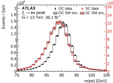
In the electron and mixed channels the lower bound is increased to 90 GeV in the three-lepton regions and to 130 GeV in the two-lepton regions. The motivation for increasing the lower mass bound in regions containing electrons is the data-driven charge misidentification background correction, where the Z → ee peak is used to measure the charge misidentification rates (described in Section5).

Differ-ences between data and MC simulation in the dielectron same-charge Z → ee peak (see Figure2) were

minimised by construction following the methodology described in Section5, and the Z → ee peak

was therefore not used in the fit. In the two-lepton regions, this bound is set to 130 GeV to completely remove the Z peak region. In the three-lepton regions, where this effect is not as strong, the bound is

relaxed to 90 GeV to reduce the statistical uncertainty of the sample. As the charge misidentification background is not present in the muon channel, there is no need to increase the lower mass bound there.

In the mixed channel, events are further divided into two categories, where the same-charge pair features different-flavour leptons or not, indicated by e±_µ±_`∓_{and e}±_e±_µ∓_{or µ}±_µ±_e∓_{, respectively.} In order to maximise the sensitivity in two-lepton and three-lepton signal regions (SR1P2L and SR1P3L), additional requirements are imposed on same-charge lepton pairs, regardless of the

fla-vour. These exploit both the boosted decay topology of the H±±resonance and the high energy of the

decay products. The same-charge lepton separation is required to be∆R(`±, `±) < 3.5. Their com-bined transverse momentum has to be pT(`±`±) > 100 GeV. 3 Finally, the scalar sum of the leptons’ transverse momenta is required to be above 300 GeV in the signal regions. In SR1P2L and SR1P3L,

the signal selection efficiency combined with the detector acceptance varies greatly with the assumed

branching ratio into light leptons. It is the highest for B(H±± → `±`±) ≈ 60% where about 40% of

signal events are selected either in SR1P2L or SR1P3L. For B(H±± →`±`±) = 100%, about 25% of

signal events are selected in either of the regions.

In the four-lepton signal region (SR2P4L), the fit variable is the average invariant mass of the two same-charge lepton pairs ¯M ≡(m+++m−−)/2. A selection on the variable∆M/ ¯M ≡ |m++− m−−|/ ¯Mis applied to reject background where the two same-charge pairs have inconsistent invariant masses. The

∆M/ ¯Mrequirement is optimised for different flavour combinations which generally feature different

mass resolutions. This selection corresponds to∆M values which are required to be below 15-50 GeV

for ¯M = 200 GeV, 30-160 GeV for ¯M = 500 GeV, and 50-500 GeV for ¯M = 1000 GeV. In the 2P4L

signal region, the fraction of signal events that are selected is approximately 50% for the B(H±± →

`±<sub>`</sub>±_{)= 100% case and lower for branching ratios into light leptons below 100%.}

The same-charge validation region (SCVR) is used to validate the data-driven fake-background es-timation and the charge misidentification effect in the electron channel. The three-lepton validation

region(3LVR) is used to validate the SM diboson background and fake events with three reconstructed

leptons with different proportions across channels. The four-lepton validation region (4LVR) is used

to validate the diboson modelling in the four-lepton region. Furthermore, the diboson control region (DBCR) is used to constrain the diboson background yield in each channel while the opposite-charge control region is used to constrain the Drell–Yan contribution in the electron channel only. The

four-lepton control region(4LCR) is used to constrain the yield of the diboson background in four-lepton

regions.

3_{The variable p}

Table 3: Summary of all regions used in the analysis. The table is split into three blocks: the upper block indicates the final states for each region, the middle block indicates the mass range of the corresponding final state, and the lower block indicates the event selection criteria for the region. The application of a selection

requirement is indicated by a check-mark (_{3). The 2P4L regions include all lepton flavour combinations. In the}

three lepton regions, `±<sub>`</sub>±_`0∓_{indicates that same-charge leptons have the same flavour, while the opposite-sign}

lepton has a different flavour.

Channel

Region Control Regions Validation Regions Signal Regions

OCCR DBCR 4LCR SCVR 3LVR 4LVR 1P2L 1P3L 2P4L Electron channel e± e∓ e± e± e∓ `±<sub>`</sub>±_{`</sub>∓<sub>`}∓ e± e± e± e± e∓ `±<sub>`</sub>±_{`</sub>∓<sub>`}∓ e± e± e± e± e∓ `±<sub>`</sub>±_{`</sub>∓<sub>`}∓ Mixed channel - e±_µ±_{`</sub>∓ e±<sub>µ</sub>± e ±<sub>µ</sub>±<sub>`}∓ `±<sub>`</sub>±_{`</sub>0∓ e ±<sub>µ</sub>± e ±<sub>µ</sub>±<sub>`}∓ `±<sub>`</sub>±<sub>`</sub>0∓ Muon channel - µ±<sub>µ</sub>±<sub>µ</sub>∓ <sub>µ</sub>±<sub>µ</sub>± <sub>µ</sub>±<sub>µ</sub>±<sub>µ</sub>∓ <sub>µ</sub>±<sub>µ</sub>± <sub>µ</sub>±<sub>µ</sub>±<sub>µ</sub>∓ m(e± e± ) [GeV] [130, 2000] [90, 200) [60, 150) [130, 200) [90, 200) [150, 200) [200, ∞) [200, ∞) [200, ∞) m(`±<sub>`</sub>± ) [GeV] - [90, 200) [130, 200) [90, 200) [200, ∞) [200, ∞) m(µ±<sub>µ</sub>± ) [GeV] - [60, 200) [60, 200) [60, 200) [200, ∞) [200, ∞) b-jet veto 3 3 3 3 3 3 3 3 3 Zveto - inverted - - 3 - - 3 3 ∆R(`±<sub>, `</sub>±<sub>) < 3.5 - - - - -</sub> -3 3 -pT(`±`±) > 100 GeV - - - 3 3 -P |pT(`)| > 300 GeV - - - 3 3 -∆M/ ¯Mrequirement - - - 3

5 Background composition and estimation

Prompt SM backgrounds in all regions are estimated using the simulated samples listed in Section3.

Prompt light leptons are defined as leptons originating from Z, W, and H boson decays or leptons from τ decays if the τ has a prompt source (e.g. Z → ττ). MC events containing at least one non-prompt or fake selected tight or loose lepton are discarded to avoid an overlap with the data-driven fake-background estimation. Prompt electrons in the remaining simulated events are corrected to account for different charge misidentification probabilities in data and simulation.

Electron charge misidentification is caused predominantly by bremsstrahlung. The emitted photon can either convert to an electron–positron pair, which happens in most of the cases, or traverse the inner detector without creating any track. In the first case, the cluster corresponding to the initial electron can be matched to the wrong-charge track, or most of the energy is transferred from one track to the other because of the photon. In case of photon emission without subsequent pair pro-duction, the electron track has usually very few hits only in the silicon pixel layers, and thus a short lever arm on its curvature. Because the electron charge is derived from the track curvature, it could be incorrectly determined while the electron energy is likely appropriate as the emitted photon de-posits all of its energy in the EM calorimeter as well. For a similar reason high-energy electrons are more often affected by charge misidentification, as their tracks are approximately straight and therefore challenging for the curvature measurement. The modelling of charge misidentification in simulation deviates from data due to the complex processes involved, which particularly rely on a very precise description of the detector material. A correction is obtained by comparing the charge misidentification probability measured in data to the one in simulation. The charge misidentification

probability is extracted by performing a likelihood fit on a dedicated Z → ee data sample (see

Fig-ure2). Electron pairs are selected around the Z boson peak and categorised in opposite-charge (OC)

and same-charge (SC) selections with the invariant mass requirements |mOC(ee) − m(Z)| < 14 GeV and |mSC(ee) − m(Z)| < 15.8 GeV, respectively. Events from contributions other than Z → ee are subtrac-ted from the peak regions. They are modelled with simulation and their normalisation is determined

from data in mass windows around the Z peak defined as 14 GeV < |mOC(ee) − m(Z)| < 18 GeV for

OC and 15.8 GeV < |mOC(ee) − m(Z)| < 31.6 GeV for SC. The number of OS and SC electron pairs

in the two regions (Ni j= N_SCi j + N_OCi j ) are then used as inputs of the likelihood fit.

75 80 85 90 95 100 105 m(ee) [GeV] 0 0.2 0.4 0.6 0.8 1 1.2 1.4 1.6 1.8 2 6 10 × Events / GeV 0 2 4 6 8 10 12 14 16 3 10 × ATLAS ee peak → Z -1 = 13 TeV, 36.1 fb s OC data SC data OC SM sim. SC SM sim.

Figure 2: Dielectron mass distributions for opposite-charge (black) and same-charge (red) pairs for data (filled circles) and MC simulation (continuous line). The latter includes a correction for charge misidentification. The hatched band indicates the statistical error and the luminosity uncertainty summed in quadrature applied to MC simulated events.

The probability to observe N_SCi j same-charge pairs is the Poisson probability:

f(N_SCi j ; λ)= λ Ni j_SCe−λ N_SCi j ! ,

with λ= Ni j(Pi(1 − Pj)+ Pj(1 − Pi)) denoting the expected number of same-charge pairs in bin (i, j), where i and j indicate the kinematic configuration of the two electrons in the pair, given the charge misidentification probabilities Pi and Pj. N_SCi j is the measured number of same-charge pairs. The formula for the negative log likelihood used in the likelihood fit is given in Eq.1:

− log L(P|NSC, N) = X i, j log(Ni j(Pi(1 − Pj)+ Pj(1 − Pi)))N i j SC− N i j (Pi(1 − Pj)+ Pj(1 − Pi)). (1)

The charge misidentification probability is parameterised as a function of electron pTand η, P(pT, η) =

σ(pT) × f (η). The binned values, σ(pT) and f (η), are free parameters in the likelihood fit. To

to unity. The charge misidentification probability is measured with the same method in a

simu-lated Z/γ∗ → ee sample and in data. The comparison of the result is shown in Figure 3. All

prompt electrons in simulated events are corrected with charge reconstruction scale factors. The scale factors are defined as P(pT, η; data)/P(pT, η; MC) if the charge is wrongly reconstructed and (1 − P(pT, η; data)) / (1 − P(pT, η; MC)) if the charge is properly reconstructed.

) T (p σ 0 0.02 0.04 0.06 0.08 0.1 0.12 0.14 0.16 0.18 0.2 ATLAS -1 = 13 TeV, 36.1 fb s ) × f(η) T (p σ ) = η , T P(p Data ee → Sherpa 2.2.1 Z [GeV] T p 40 50 100 200 300 400 Data / MC 0.6 0.8 1.0 1.2 1.4 (a) ) η f( 2 − 10 1 − 10 1 10 ATLAS -1 = 13 TeV, 36.1 fb s ) × f(η) T (p σ ) = η , T P(p Data ee → Sherpa 2.2.1 Z | η | 0 0.5 1 1.5 2 2.5 Data / MC 0.6 0.8 1.0 1.2 1.4 (b)

Figure 3: Comparison of the factors composing the charge misidentification probability P(pT, η) = σ(pT) × f (η)

measured in data and in simulation using the likelihood fit in the Z/γ∗_{→ ee region. The area of the distribution}

describing f (η) was set to unity (see text for details). Error bars correspond to the statistical uncertainties

estimated with the likelihood fit. Plot(a)shows the charge misidentification probability component as a function

of pTand plot(b)shows the component as a function of |η|.

The fake-lepton background is estimated with a data-driven approach, the so-called ‘fake factor’

method, as described in Ref. [27]. The b-jet veto significantly reduces fake leptons from

heavy-flavour decays. Most of the fake leptons still passing the analysis selection originate from in-flight decays of mesons inside jets, jets misreconstructed as electrons, and conversions of initial- and final-state radiation photons. The fake factor method provides an estimation of events with fake leptons in analysis regions by extrapolating the yields from the so-called ‘side-band regions’. For each analysis region a corresponding side-band region is defined. It requires exactly the same selection and lepton multiplicity except that at least one lepton must fail to satisfy the tight identification criteria. The ratio of tight to loose leptons is measured in dedicated ‘fake-enriched regions’. It is determined as a func-tion of lepton flavour, pT, and η, and referred to as the ‘fake factor’ (F(pT, η, flavour)). It describes the probability for a fake lepton to be identified as a tight lepton. The definitions of the fake-enriched

regions for the electron and muon channels are reported in Table4. In the measurement of the fake

factor, a requirement on the unbalanced momentum in the transverse plane of the event, E_Tmiss, is

im-posed to reject W+ jets events and to further enrich the regions with fake leptons. The fake factor

method relies on the assumption that no prompt leptons appear in the fake-enriched samples. This assumption is not fully correct with the imposed selection. Therefore, the number of residual prompt leptons in the fake-enriched regions is estimated using simulation and subtracted from the numbers of tight and loose leptons used to measure the fake factors.

Table 4: Selection criteria defining the fake-enriched regions used to measure the ratio of the numbers of tight and loose leptons, the so-called fake factor, for the electron and muon channels.

Selection for fake-enriched regions

Muon channel Electron channel

Single-muon trigger Single-electron trigger

b-jet veto b-jet veto

One muon and one jet One electron

pT(jet) > 35 GeV Number of tight electrons< 2

∆φ(µ, jet) > 2.7 m(ee) < [71.2, 111.2] GeV

Emiss_T < 40 GeV Emiss_T < 25 GeV

The number of events in the analysis regions containing at least one fake lepton, Nfake, is estimated from the side-bands. Data are weighted with fake factors according to the loose lepton multiplicity of the region: Nfake = N_SBdata X i=1 (−1)NL,i+1 NL,i Y l=1 Fl − N_SBMC X i=1 (−1)NL,i+1 NL,i Y l=1 Fl,

with N_SBdatadenoting the number of data events in the side-band, NL,iis the loose lepton multiplicity in the i-th event of the side-band region and l indicates the loose lepton. The contamination of prompt leptons in the side-band region is subtracted using simulated events, denoted by N_SBMC.

Dedicated two-lepton and three-lepton validation regions, defined in Table 3, are used to verify the

data-driven fake-lepton estimation in regions as similar to the signal regions as possible. They are designed to contain only a negligible number of signal events. Orthogonality between signal and validation regions is ensured by requiring the invariant mass of the same-charge lepton pair m(`±`±) to be less than 200 GeV in the validation regions. Furthermore, diboson modelling and the elec-tron charge misidentification backgrounds are tested. Each background estimation is validated in the corresponding regions, defined to be enriched in the given contribution.

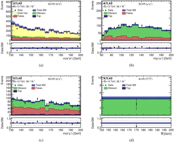
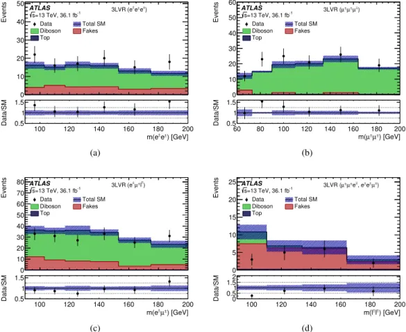
Figures4and5present all validation regions sensitive to different background sources: same-charge

two-lepton validation regions (SCVR) for testing the charge misidentification background model-ling and fake-background predictions, and three-lepton and four-lepton validation regions (3LVR and 4LVR) for testing the diboson modelling. Good background modelling is observed in all these re-gions.

Events 0 100 200 300 400 500 600 700 800 _ATLAS -1 =13 TeV, 36.1 fb s ) ± e ± SCVR (e Data Total SM Drell-Yan Diboson Fakes Top ) [GeV] ± e ± m(e 130 140 150 160 170 180 190 200 Data/SM 0.5 1 1.5 (a) Events 0 50 100 150 200 250 ATLAS -1 =13 TeV, 36.1 fb s ) ± µ ± µ SCVR ( Data Total SM Diboson Fakes Top ) [GeV] ± µ ± µ m( 60 80 100 120 140 160 180 200 Data/SM 0.5 1 1.5 (b) Events 0 20 40 60 80 100 120 140 160 180 200 220 ATLAS -1 =13 TeV, 36.1 fb s ) ± µ ± SCVR (e Data Total SM Diboson Fakes Top ) [GeV] ± µ ± m(e 130 140 150 160 170 180 190 200 Data/SM 0.5 1 1.5 (c) Events 0 2 4 6 8 10 ATLAS -1 =13 TeV, 36.1 fb s ) ± l ± l ± l ± 4LVR (l Data Total SM Diboson Top [GeV] M 150 155 160 165 170 175 180 185 190 195 200 Data/SM 0.5 1 1.5 (d)

Figure 4: Distributions of dilepton mass for data and SM background predictions in two- and four-lepton

valid-ation regions:(a)the electron–electron,(b)the muon–muon, and(c)the electron–muon two-lepton validation

regions, as well as(d)the four-lepton validation region. The hatched bands include all systematic uncertainties

Events 0 10 20 30 40 50 ATLAS -1 =13 TeV, 36.1 fb s ) ± e ± e ± 3LVR (e Data Total SM Diboson Fakes Top ) [GeV] ± e ± m(e 100 120 140 160 180 200 Data/SM 0.5 1 1.5 (a) Events 0 10 20 30 40 50 60 ATLAS -1 =13 TeV, 36.1 fb s ) ± µ ± µ ± µ 3LVR ( Data Total SM Diboson Fakes Top ) [GeV] ± µ ± µ m( 60 80 100 120 140 160 180 200 Data/SM 0.5 1 1.5 (b) Events 0 10 20 30 40 50 60 70 80 ATLAS -1 =13 TeV, 36.1 fb s ) ± l ± µ ± 3LVR (e Data Total SM Diboson Fakes Top ) [GeV] ± µ ± m(e 100 120 140 160 180 200 Data/SM 0.5 1 1.5 (c) Events 0 5 10 15 20 25 ATLAS -1 =13 TeV, 36.1 fb s ) ± µ ± e ± , e ± e ± µ ± µ 3LVR ( Data Total SM Diboson Fakes Top ) [GeV] ± l ± m(l 100 120 140 160 180 200 Data/SM 0.50 1 1.52 (d)

Figure 5: Distribution of dilepton mass for data and SM background predictions in three-lepton validation

regions: (a)the three-electron validation region, (b)the three-muon validation region, (c)the 3LVR with an

electron–muon same-charge pair (e±_µ±_`∓_{), and(d)the 3LVR with a same-flavour same-charge pair (e}±_e±_µ∓_or

µ±_µ±_e∓_{). The hatched bands include all systematic uncertainties post-fit, with the correlations between various} sources taken into account.

6 Systematic uncertainties

Several sources of systematic uncertainty are accounted for in the analysis. These correspond to

experimental and theoretical sources affecting both background and signal predictions. All considered

sources of systematic uncertainty affect the total event yield, and all except the uncertainties on the luminosity and cross section also affect the distributions of the variables used in the fit (Section7). The cross-sections used to normalise the simulated samples are varied to account for the scale and

PDF uncertainties in the cross-section calculation. The variation is 6% for diboson production [77],

13% for t¯tW production, 12% for t¯tZ production, and 8% for t¯tH production [49]. The theoretical

uncertainty in the Drell–Yan background is estimated by PDF eigenvector variations of the

nom-inal PDF set, variations of PDF scale, αS, electroweak corrections, and photon-induced corrections.

The effect of the PDF choice is considered by comparing the nominal PDF set to several others,

namely CT10NNLO [62], MMHT14 [78], NNPDF3.0 [43], ABM12 [79], HERAPDF2.0 [80, 81],

and JR14 [82]. An envelope is constructed by taking into account the largest deviations from the nom-inal choice. The predominant prompt background, arising from diboson production, is assigned an additional theoretical uncertainty by comparing the nominal Sherpa 2.2.1 prediction with the Powheg prediction. This uncertainty varies from 5% to 10%. Furthermore, the theoretical uncertainty in the NLO cross-section for pp → H++H−−is reported to be about 15% [9]. It includes the renormalization and factorization scale dependence and the uncertainty in the parton densities. Lastly, the theoretical

uncertainty in the simulated pp → H++H−− events is assessed by varying the A14 parameter set in

Pythia 8.186 and choosing alternative PDFs CTEQ6L1 and CT09MC1 [83]. The impact on the signal

acceptance is found to be negligible.

A significant contribution arises from the statistical uncertainty in the MC samples and data sideband regions. Analysis regions have a very restrictive selection and only a small fraction of the initially generated MC events remains after applying all requirements. The statistical uncertainty varies from 5% to 40% depending on the signal region.

Experimental systematic uncertainties due to different reconstruction, identification, isolation, and trigger efficiencies of leptons in data compared to simulation are estimated by varying the correspond-ing scale-factors. They are at most 3% and less significant than the other systematic uncertainties and MC statistical uncertainties. The same is true for lepton energy or momentum calibration.

The experimental uncertainty related to the charge misidentification probability of electrons arises from the statistical uncertainty of both the data and the simulated sample of Z/γ∗→ ee events used to measure this probability. The uncertainty ranges between 10% and 20% as a function of the electron pTand η. Possible systematic effects were investigated by altering the selection requirements imposed

on the invariant mass used to select Z/γ∗→ ee events analysed to measure the misidentification

prob-ability. The effects estimated with this method are found to be negligible compared to the statistical uncertainty.

The experimental systematic uncertainty in the data-driven estimate of the fake-lepton background is evaluated by varying the nominal fake factor to account for different effects. The Emiss_T requirement

is altered to consider variations in the W+ jets composition. The flavour composition of the fakes is

investigated by requiring an additional recoiling jet in the electron channel and changing the definition of the recoiling jet in the muon channel. Furthermore, the transverse impact parameter criterion for tight muons (defined in Section4.1) is varied by one standard deviation. Finally, in the fake-enriched

regions, the normalisation of the subtracted simulated samples, to remove the prompt lepton compon-ent, is altered within its uncertainties. This accounts for uncertainties related to the luminosity, the cross-section, and the corrections applied to simulation-based predictions. The statistical uncertainty in the fake factors is added in quadrature to the total systematic error. The uncertainty ranges between

10% and 20% across all pTand η bins.

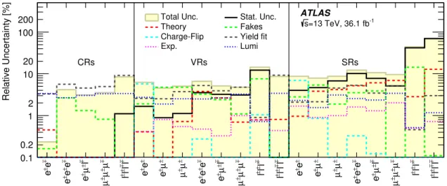
The total relative systematic uncertainty after the fit (Section7), and its breakdown into components,

is presented in Figure 6. All experimental systematic uncertainties discussed here affect the signal

samples as well as the background.

± e ± e ± e ± e ± e ± _l ±_µ ± e ± µ ±_µ ± µ ± _l ± l ± _l ± _l ±_e ± e ±_µ ± e ±_µ ± µ ± e ± e ± e ± _l ±_µ ± e ± µ ±_µ ± µ ± l’ ± _l ± _l ± _l ± l ± _l ± _l ±_e ± e ±_µ ± e ±_µ ± µ ± e ± e ± e ± _l ±_µ ± e ± µ ±_µ ± µ ± l’ ±_l ±_l ± _l ± l ± _l ± _l Relative Uncertainty [%] 0.1 0.2 1 2 10 20 100 200 CRs VRs SRs

Total Unc. Stat. Unc.

Theory Fakes

Charge-Flip Yield fit

Exp. Lumi

ATLAS

-1

=13 TeV, 36.1 fb s

Figure 6: Relative uncertainties in the total background yield estimation after the fit. ‘Stat. Unc.’ corresponds to reducible and irreducible background statistical uncertainties. ‘Yield fit’ corresponds to the uncertainty arising from fitting the yield of diboson and Drell–Yan backgrounds. ‘Lumi’ corresponds to the uncertainty in the luminosity. ‘Theory’ indicates the theoretical uncertainty in the physics model used for simulation (e.g.

cross-sections). ‘Exp.’ indicates the uncertainty in the simulation of electron and muon efficiencies (e.g. trigger,

identification). ‘Fakes’ is the uncertainty associated with the model of the fake background. Individual uncer-tainties can be correlated, and do not necessarily add in quadrature to the total background uncertainty, which is indicated by ‘Total Unc.’.

7 Statistical analysis and results

The statistical analysis package HistFitter [84] was used to implement a maximum-likelihood fit of

the dilepton invariant mass distribution in all control and signal regions, and the ¯Mdistribution in four-lepton regions to obtain the numbers of signal and background events. The likelihood is the product of a Poisson probability density function describing the observed number of events and Gaussian distributions to constrain the nuisance parameters associated with the systematic uncertainties. The widths of the Gaussian distributions correspond to the magnitudes of these uncertainties, whereas Poisson distributions are used for MC simulation statistical uncertainties. Furthermore, additional free parameters are introduced for the Drell–Yan and the diboson background contributions, to fit their yields in the analysis regions. Fitting the yields of the largest backgrounds reduces the systematic uncertainty in the predicted yield from SM sources. The fitted normalisations are compatible with their SM predictions within the uncertainties. The diboson yield is described by four free parameters,

each corresponding to a different diboson region: electron channel, muon channel, mixed channel, and the four-lepton channel. After the fit, the compatibility between the data and the expected background was assessed. For various branching ratio assumptions, 95% CL upper limits were set on the pp → H++H−−cross-section using the CLsmethod [85].

7.1 Fit results

The observed and expected yields in all control, validation, and signal regions used in the analysis

are presented in Figure7and summarised in Tables5to7. No significant excess is observed in any

of the signal regions. Correlations between various sources of uncertainty are evaluated and used to estimate the total uncertainty in the SM background prediction. Two- and four-lepton signal regions are presented in Figure8and three-lepton signal regions are presented in Figure9. In the four-lepton

signal region only one data event is observed. It is an e+µ+e−µ− event with invariant masses of

228 GeV and 207 GeV for the same-charge lepton pairs.

Events 1 − 10 1 10 2 10 3 10 4 10 5 10 CRs VRs SRs ATLAS -1 =13 TeV, 36.1 fb s Data Total SM Drell-Yan Diboson Fakes Top ± e ± e ± e ± e ±_e ± _l ±_µ ± e ± µ ±_µ ± µ ± l ± l ± _l ± _l ± e ± e ±_µ ± e ±_µ ± µ ± e ± e ±_e ± _l ±_µ ± e ± µ ±_µ ± µ ± l’ ± _l ± _l ± _l ± l ± _l ± _l ± e ± e ±_µ ± e ±_µ ± µ ± e ± e ±_e ± _l ±_µ ± e ± µ ±_µ ± µ ± l’ ±_l ±_l ± _l ± l ± _l ± _l Data/SM 0.5 1 1.5

Figure 7: Number of observed and expected events in the control, validation, and signal regions for all channels considered. The background expectation is the result of the fit described in the text. The hatched bands include all systematic uncertainties post-fit with the correlations between various sources taken into account. The notation `±<sub>`</sub>0±_{`</sub>∓<sub>indicates that the same-charge leptons have different flavours and `}±_{`</sub>±<sub>`}0∓_{indicates that}

same-charge leptons have the same flavour, while the opposite-same-charge lepton has a different flavour.

The likelihood fit to the two-, three-, and four-lepton control and signal regions was designed to fully

exploit the pair production of the H±± boson with its boosted topology and lepton multiplicity. For

B(H±± → `±`±) = 100% the production cross-section is excluded down to 0.1 fb, corresponding to

3–4 signal events, which is the theoretical limit of a 95% CL exclusion. Some representative

cross-section upper limits as a function of the H±± boson mass are presented in Figure10, for different

combinations of the branching ratios for decay into light-lepton pairs.

The final result of the fit is a lower limit on the two-dimensional grid of the H±± boson mass for any combination of light lepton branching ratios that sum to a certain value. The fit was performed for

values of B(H±± →`±`±) from 1% to 5% in 1% intervals, and from 10% to 100% in 10% intervals.

Expected limits for B(H±± → `±`±) = 100% are presented in Figure11for H±±_L and in Figure12

Table 5: The number of predicted background events in control regions after the fit, compared to the data. Uncertainties correspond to the total uncertainties in the predicted event yields, and are smaller for the total than the sum of the components in quadrature due to correlations between these components. Due to rounding

the totals can differ from the sums of components. Background processes with a negligible yield are marked

with the en dash (–).

OCCR DBCR DBCR DBCR 4LCR e±_e∓ _e±_e±_e∓ _e±_µ±_{`</sub>∓ <sub>µ</sub>±<sub>µ</sub>±<sub>µ</sub>∓ <sub>`}±_{`</sub>±<sub>`}∓_`∓ Observed events 184 569 576 1025 797 140 Total background 184 570 ± 430 574 ± 24 1025 ± 32 797 ± 28 140 ± 12 Drell–Yan 169 980 ± 990 – – – – Diboson 5060 ± 900 449 ± 28 909 ± 35 775 ± 29 138 ± 12 Fakes 2340 ± 300 123 ± 15 113 ± 14 19.9 ± 6.5 1.31 ± 0.16 Top 7200 ± 250 1.58 ± 0.06 2.90 ± 0.11 2.04 ± 0.08 0.37 ± 0.01

three specific decay scenarios to only e±e±, µ±µ±, and e±µ±, are considered and the minimum limit

for each value of B(H±± →`±`±) is given. The minimum limit is obtained by taking, for each value

of B(H±± → `±`±), the least stringent limit for any combination of branching ratios that sum to

B(H±± → `±`±). The lower mass limits for these four cases are similar, which indicates that the

analysis is almost equally sensitive to each decay channel.

The observed lower mass limits vary from 770 GeV to 870 GeV for H_L±±with B(H±± →`±`±)= 100%

and are above 450 GeV for B(H±± →`±`±) ≥ 10%. For H±±_R the lower mass limits vary from 660 GeV

Table 6: The number of predicted background events in two-lepton and four-lepton validation regions (top) and three-lepton validation regions (bottom) after the fit, compared to the data. Uncertainties correspond to the total uncertainties in the predicted event yields, and are smaller for the total than the sum of the components in

quadrature due to correlations between these components. Due to rounding the totals can differ from the sums

of components. Background processes with a negligible yield are marked with the en dash (–).

SCVR SCVR SCVR 4LVR e±_e± _e±_µ± _µ±_µ± _{`</sub>±<sub>`}±_{`</sub>∓<sub>`}∓ Observed events 3237 1162 1006 3 Total background 3330 ± 210 1119 ± 51 975 ± 50 4.62 ± 0.40 Drell–Yan 2300 ± 190 – – – Diboson 319 ± 25 547 ± 23 719 ± 30 4.59 ± 0.4 Fakes 640 ± 65 502 ± 54 249 ± 47 – Top 71.5 ± 6.8 70.5 ± 2.6 6.93 ± 0.27 0.033 ± 0.001 3LVR 3LVR 3LVR 3LVR e±_e±_e∓ _e±_µ±_`∓ _µ±_µ±_µ∓ _µ±_µ±_e∓_{, e}±_e±_µ∓ Observed events 108 180 126 16 Total background 88.1 ± 5.8 192.9 ± 9.9 107.0 ± 5.1 27.0 ± 3.9 Diboson 64.4 ± 5.8 147.3 ± 9.0 100.9 ± 5.0 4.72 ± 0.79 Fakes 23.3 ± 3.0 43.9 ± 4.9 5.3 ± 1.2 21.3 ± 3.4 Top 0.50 ± 0.03 1.73 ± 0.09 0.82 ± 0.05 1.01 ± 0.15

Table 7: The number of predicted background events in two-lepton and four-lepton signal regions (top) and three-lepton signal regions (bottom) after the fit, compared to the data. Uncertainties correspond to the total uncertainties in the predicted event yields, and are smaller for the total than the sum of the components in

quadrature due to correlations between these components. Due to rounding the totals can differ from the sums

of components. Background processes with a negligible yield are marked with the en dash (–).

SR1P2L SR1P2L SR1P2L SR2P4L e±_e± _e±_µ± _µ±_µ± _{`</sub>±<sub>`}±_{`</sub>∓<sub>`}∓ Observed events 132 106 26 1 Total background 160 ± 14 97.1 ± 7.7 22.6 ± 2.0 0.33 ± 0.23 Drell–Yan 70 ± 10 – – – Diboson 30.5 ± 3.0 40.4 ± 4.5 20.3 ± 1.8 0.11 ± 0.06 Fakes 52.2 ± 5.0 53.1 ± 5.8 1.94 ± 0.47 0.22 ± 0.19 Top 7.20 ± 0.97 3.62 ± 0.53 0.42 ± 0.03 0.007 ± 0.002 SR1P3L SR1P3L SR1P3L SR1P3L e±_e±_e∓ _e±_µ±_`∓ _µ±_µ±_µ∓ _µ±_µ±_e∓_{, e}±_e±_µ∓ Observed events 11 23 13 2 Total background 13.0 ± 1.6 34.2 ± 3.6 13.2 ± 1.3 3.1 ± 1.4 Diboson 9.5 ± 1.3 23.1 ± 2.9 13.1 ± 1.3 0.27 ± 0.14 Fakes 3.3 ± 0.67 10.7 ± 1.7 – 2.6 ± 1.2 Top 0.14 ± 0.02 0.45 ± 0.04 0.12 ± 0.01 0.19 ± 0.08

Events 0 10 20 30 40 50 60 70 _ATLAS -1 =13 TeV, 36.1 fb s ) ± e ± SR1P2L (e Data Total SM Drell-Yan Diboson Fakes Top (X) = 80% B ) = 20%, ± e ± (e B ) = 450 GeV ± ± m(H (X) = 50% B ) = 50%, ± e ± (e B ) = 650 GeV ± ± m(H (X) = 50% B ) = 50%, ± e ± (e B ) = 850 GeV ± ± m(H ) [GeV] ± e ± m(e 300 400 500 1000 2000 Data/SM 0.50 1 1.52 (a) Events 0 2 4 6 8 10 12 14 16 18 20 ATLAS -1 =13 TeV, 36.1 fb s ) ± µ ± µ SR1P2L ( Data Total SM Diboson Fakes Top (X) = 80% B ) = 20%, ± µ ± µ ( B ) = 450 GeV ± ± m(H (X) = 50% B ) = 50%, ± µ ± µ ( B ) = 650 GeV ± ± m(H (X) = 50% B ) = 50%, ± µ ± µ ( B ) = 850 GeV ± ± m(H ) [GeV] ± µ ± µ m( 300 400 500 1000 2000 Data/SM 0.50 1 1.52 (b) Events 0 10 20 30 40 50 ATLAS -1 =13 TeV, 36.1 fb s ) ± µ ± SR1P2L (e Data Total SM Diboson Fakes Top (X) = 80% B ) = 20%, ± µ ± (e B ) = 450 GeV ± ± m(H (X) = 50% B ) = 50%, ± µ ± (e B ) = 650 GeV ± ± m(H (X) = 50% B ) = 50%, ± µ ± (e B ) = 850 GeV ± ± m(H ) [GeV] ± µ ± m(e 300 400 500 1000 2000 Data/SM 0.50 1 1.52 (c) Events 3 − 10 2 − 10 1 − 10 1 10 2 10 3 10 4 10 5 10 ATLAS -1 =13 TeV, 36.1 fb s ) ± l ± l ± l ± SR2P4L (l Data Total SM Diboson Fakes Top ) = 100% ± µ ± µ ( B ) = 450 GeV ± ± m(H ) = 100% ± µ ± µ ( B ) = 650 GeV ± ± m(H ) = 100% ± µ ± µ ( B ) = 850 GeV ± ± m(H [GeV] M 200 400 600 800 1000 1200 Data/SM 0.50 1 1.52 (d)

Figure 8: Distributions of m(`±<sub>`</sub>±_{) in representative signal regions, namely(a)the electron–electron two-lepton}

signal region (SR1P2L),(b)the muon–muon two-lepton signal region (SR1P2L),(c)the electron–muon

two-lepton signal region (SR1P2L), and(d)the four-lepton signal region (SR2P4L). The hatched bands include all

systematic uncertainties post-fit with the correlations between various sources taken into account. The solid

coloured lines correspond to signal samples, normalised using the theory cross-section, with the H±±_{mass and}

Events 0 2 4 6 8 10 12 14 16 18 ATLAS -1 =13 TeV, 36.1 fb s ) ± e ± e ± SR1P3L (e Data Total SM Diboson Fakes Top ) = 100% ± e ± (e B ) = 450 GeV ± ± m(H ) = 100% ± e ± (e B ) = 650 GeV ± ± m(H ) = 100% ± e ± (e B ) = 850 GeV ± ± m(H ) [GeV] ± e ± m(e 300 400 500 1000 2000 Data/SM 0.50 1 1.52 (a) Events 0 2 4 6 8 10 12 14 16 18 20 ATLAS -1 =13 TeV, 36.1 fb s ) ± µ ± µ ± µ SR1P3L ( Data Total SM Diboson Top ) = 100% ± µ ± µ ( B ) = 450 GeV ± ± m(H ) = 100% ± µ ± µ ( B ) = 650 GeV ± ± m(H ) = 100% ± µ ± µ ( B ) = 850 GeV ± ± m(H ) [GeV] ± µ ± µ m( 300 400 500 1000 2000 Data/SM 0.50 1 1.52 (b) Events 0 5 10 15 20 25 30 35 40 45 ATLAS -1 =13 TeV, 36.1 fb s ) ± l ± µ ± SR1P3L (e Data Total SM Diboson Fakes Top ) = 100% ± µ ± (e B ) = 450 GeV ± ± m(H ) = 100% ± µ ± (e B ) = 650 GeV ± ± m(H ) = 100% ± µ ± (e B ) = 850 GeV ± ± m(H ) [GeV] ± µ ± m(e 300 400 500 1000 2000 Data/SM 0.50 1 1.52 (c) Events 0 2 4 6 8 10 12 ATLAS -1 =13 TeV, 36.1 fb s ) ± µ ± e ± , e ± e ± µ ± µ SR1P3L ( Data Total SM Diboson Fakes Top ) = 25% ± µ ± µ ( B ) = ± e ± (e B ) = 450 GeV ± ± m(H ) = 50% ± µ ± µ ( B ) = ± e ± (e B ) = 650 GeV ± ± m(H ) = 50% ± µ ± µ ( B ) = ± e ± (e B ) = 850 GeV ± ± m(H ) [GeV] ± l ± m(l 200 400 600 800 1000 1200 1400 1600 1800 2000 Data/SM 0.50 1 1.52 (d)

Figure 9: Distributions of m(`±<sub>`</sub>±_{) in three-lepton signal regions, namely(a)the three-electron SR (SR1P3L),(b)}

the three-muon SR (SR1P3L),(c)the SR1P3L with an electron–muon same-charge pair (e±_µ±_`∓_{), and(d)the}

SR1P3L with a same-flavour same-charge pair (e±_e±_µ∓_{or µ}±_µ±_e∓_{). The hatched bands include all systematic}

uncertainties post-fit with the correlations between various sources taken into account. The solid coloured lines

correspond to signal samples, normalised using the theory cross-section, with the H±±_{mass and decay modes}

) [GeV] ± ± m(H 300 400 500 600 700 800 900 1000 1100 1200 [fb]) --H ++ H → (pp σ 2 − 10 1 − 10 1 10 2 10 3 10 Observed 95% CL limit Expected 95% CL limit σ 1 ± Expected limit σ 2 ± Expected limit ) --L H ++ L H → (pp σ ) --R H ++ R H → (pp σ ATLAS -1 = 13 TeV, 36.1 fb s )=100% ± e ± (e B )=0% ± µ ± (e B )=0% ± µ ± µ ( B (a) ) [GeV] ± ± m(H 300 400 500 600 700 800 900 1000 1100 1200 [fb]) --H ++ H → (pp σ 2 − 10 1 − 10 1 10 2 10 3 10 Observed 95% CL limit Expected 95% CL limit σ 1 ± Expected limit σ 2 ± Expected limit ) --L H ++ L H → (pp σ ) --R H ++ R H → (pp σ ATLAS -1 = 13 TeV, 36.1 fb s )=0% ± e ± (e B )=0% ± µ ± (e B )=100% ± µ ± µ ( B (b) ) [GeV] ± ± m(H 300 400 500 600 700 800 900 1000 1100 1200 [fb]) --H ++ H → (pp σ 2 − 10 1 − 10 1 10 2 10 3 10 Observed 95% CL limit Expected 95% CL limit σ 1 ± Expected limit σ 2 ± Expected limit ) --L H ++ L H → (pp σ ) --R H ++ R H → (pp σ ATLAS -1 = 13 TeV, 36.1 fb s )=0% ± e ± (e B )=100% ± µ ± (e B )=0% ± µ ± µ ( B (c) ) [GeV] ± ± m(H 300 400 500 600 700 800 900 1000 1100 1200 [fb]) --H ++ H → (pp σ 2 − 10 1 − 10 1 10 2 10 3 10 Observed 95% CL limit Expected 95% CL limit σ 1 ± Expected limit σ 2 ± Expected limit ) --L H ++ L H → (pp σ ) --R H ++ R H → (pp σ ATLAS -1 = 13 TeV, 36.1 fb s )=30% ± e ± (e B )=40% ± µ ± (e B )=30% ± µ ± µ ( B (d)

Figure 10: Upper limit on the cross-section for pp → H++H−−_{for several branching ratio values presented in the}

form B(ee)/B(eµ)/B(µµ): (a)100%/0%/0%,(b)0%/0%/100%,(c)0%/100%/0%, and(d)30%/40%/30%.

The theoretical uncertainty in the cross-section for pp → H++H−− _{is presented with the shaded band around}

the central value.

) limit [GeV]_L expected 95% CL m(H 840 845 850 855 860 850 849 847 846 846 847 848 849 851 854 857 848 847 845 844 844 844 845 847 849 852 846 845 843 842 842 842 843 845 847 845 844 842 841 841 841 842 843 845 843 841 840 840 840 841 845 843 842 841 841 840 846 845 843 843 842 849 847 846 845 852 851 850 857 856 863 ) [%] ± e ± e → ± ± L (H B 0 20 40 60 80 100 ) [%] ± µ ± µ → ±± L (H B 0 20 40 60 80 100 ATLAS -1 =13 TeV, 36.1 fb s )=100% ± l ± l → ± ± L (H B (a) ) limit [GeV]_L observed 95% CL m(H 780 800 820 840 860 875 862 848 833 818 803 791 781 774 770 768 871 859 845 831 816 802 790 779 771 765 868 856 843 829 814 800 788 777 764 864 853 840 826 812 798 786 766 860 849 837 824 810 797 774 856 846 834 822 809 786 852 843 832 822 801 849 841 832 816 847 840 828 846 838 846 ) [%] ± e ± e → ± ± L (H B 0 20 40 60 80 100 ) [%] ± µ ± µ → ±± L (H B 0 20 40 60 80 100 ATLAS -1 =13 TeV, 36.1 fb s )=100% ± l ± l → ± ± L (H B (b)

Figure 11: The (a)expected and (b) observed lower limits on the H±±

L boson mass for all branching ratio

) limit [GeV] R expected 95% CL m(H 725 730 735 740 745 738 736 734 732 731 730 731 732 734 737 743 736 734 731 729 728 728 729 730 732 736 734 732 729 727 726 726 726 728 731 732 730 727 726 725 724 725 726 731 729 726 725 724 725 724 730 728 726 725 724 723 731 729 727 726 725 732 730 729 728 735 733 732 739 738 745 ) [%] ± e ± e → ± ± R (H B 0 20 40 60 80 100 ) [%] ± µ ± µ → ±± R (H B 0 20 40 60 80 100 ATLAS -1 =13 TeV, 36.1 fb s )=100% ± l ± l → ± ± R (H B (a) ) limit [GeV] R observed 95% CL m(H 660 680 700 720 740 760 761 750 735 721 706 692 680 670 664 660 658 757 746 732 718 704 691 679 669 662 656 752 741 728 715 702 689 678 669 657 747 737 725 712 699 688 677 661 741 732 721 709 697 700 668 736 728 718 707 696 678 732 724 715 705 689 728 721 714 699 726 720 709 724 717 723 ) [%] ± e ± e → ± ± R (H B 0 20 40 60 80 100 ) [%] ± µ ± µ → ±± R (H B 0 20 40 60 80 100 ATLAS -1 =13 TeV, 36.1 fb s )=100% ± l ± l → ± ± R (H B (b)

Figure 12: The (a)expected and (b) observed lower limits on the H±±

R boson mass for all branching ratio

combinations that sum to 100%.

) [GeV] ± ± L m(H 300 400 500 600 700 800 900 1000 X) [%] → ±± L (H B ) = 1-±_e ± e → ±± L (H B 1 2 3 4 10 20 30 40 100 Observed 95% CL limit Expected 95% CL limit σ 1 ± Expected limit σ 2 ± Expected limit ATLAS -1 =13 TeV, 36.1 fb s ) ± ± L lower limit of m(H (a) ) [GeV] ± ± L m(H 300 400 500 600 700 800 900 1000 X) [%] → ±± L (H B ) = 1-±_µ ±_µ → ±± L (H B 1 2 3 4 10 20 30 40 100 Observed 95% CL limit Expected 95% CL limit σ 1 ± Expected limit σ 2 ± Expected limit ATLAS -1 =13 TeV, 36.1 fb s ) ± ± L lower limit of m(H (b) ) [GeV] ± ± L m(H 300 400 500 600 700 800 900 1000 X) [%] → ±± L (H B ) = 1-±_µ ± e → ±± L (H B 1 2 3 4 10 20 30 40 100 Observed 95% CL limit Expected 95% CL limit σ 1 ± Expected limit σ 2 ± Expected limit ATLAS -1 =13 TeV, 36.1 fb s ) ± ± L lower limit of m(H (c) ) [GeV] ± ± L m(H 300 400 500 600 700 800 900 1000 X) [%] → ±± L (H B ) = 1-±l ± _l → ±± L (H B 1 2 3 4 10 20 30 40 100 Observed 95% CL limit Expected 95% CL limit σ 1 ± Expected limit σ 2 ± Expected limit ATLAS -1 =13 TeV, 36.1 fb s ) ± ± L lower limit of m(H minimum limit (d)

Figure 13: Lower limit on the H±±_L boson mass as a function of the branching ratio B(H±±_L →`±<sub>`</sub>±_{). Several}

cases are presented:(a)H±±_L decays only into electrons and "X",(b)H_L±±decays only into muons and "X", and

(c)H±±

L decays only into electron–muon pairs and "X", with "X" not entering any of the signal regions. Plot(d)

shows the minimum observed and expected limit as a function of B(H±±

L →`