A Dissertation Submitted to
Post Graduate Department of Earthquake Engineering,
Faculty of Science and Technology,
Khwopa Engineering College,
Purbanchal University, Bhaktapur, Nepal
By
Hem Chandra Chaulagain
Registration No.: 035-3-3-04312-2007
In
Partial Fulfillment of Requirements for
The Master of Engineering in Earthquake
i
Er. Radha Krishna Mallik who made the otherwise impossible task an easy one by providing me valuable materials, guidance and suggestions and thus built stairs of hope and confidence by which I was able to complete this research work.
I am, indeed, thankful to Dr. Deepak Chamalagain, Er. Sajana Suwal, Dr. Bijaya Jaishi, Dr. Govinda Pd. Lamichhane, Dr. Jishnu Subedi, Er. Prachanda Man Pradhan, Er. Alin Chandra Shakya, Er. Hima Shrestha, Mr. Arjun Kr. Gaire, Er. Ganesh Ram Knemaphuki, Er.Chandra Kiran Kawan and Er. Sanjeev Prajapati who encouraged me both directly and indirectly and anticipated the completion of this work.
My sincere thanks go to all of my friends for their suggestions and support during the entire research period.
Last, but not least, I am obliged to my parents, my brother Sitaram and my beloved Kalpana for their continuous encouragement and support during my study period.
ii
overstrength factors are estimated by analyzing the buildings using non-linear pushover analysis for 12 engineered designed RC buildings of various characteristics representing a wide range of RC buildings in Kathmandu valley. Finally, the response reduction factor of RC building in Kathmandu valley is evaluated by using the relation of ductility and overstrength factor.
iii ACKNOWLEDGEMENT...III ABSTRACT...IV TABLE OF CONTENTS...V LIST OF FIGURES...IX LIST OF TABLES...X ANNEXES...XI LIST OF ABBREVIATIONS...XII 1 INTRODUCTION...1
1.1 Background of the Study ...1
1.1.1 Seismic Hazard of Nepal and Kathmandu Valley ... 1
1.1.2 Trend of Building Design and Construction ... 2
1.1.3 Research need... 4
2 OBJECTIVES, APPROACHES AND METHODOLOGIES ...5
2.1 Objective of the Study...5
2.2 Study Approaches ...5
2.3 Research Methodology...6
2.3.1 Review and study of engineered design buildings in Kathmandu valley ... 6
2.3.2 Selection of sample building for response reduction factor (R) study ... 6
2.3.3 Review of response reduction factor methodologies ... 7
iv
3.3 Previous Studies on calculation of Response Reduction Factors ... 12
3.4.1 Overstrength ... 13
3.4.2 Previous studies on calculation of overstrength ...14
3.5 Ductility Reduction Factor ...16
3.5.1 Terms used in ductility reduction factors ... 16
3.5.2 Previous studies on Calculation of Ductility Reduction Factors ... 19
3.5.3 Ductility of unconfined beam sections. ... 21
3.6 Redundancy Factor... 23
3.7 Codal provisions for reduction factors: ... 24
3.7.1 Response Reduction Factor as per ATC-19... 24
3.7.2 Response Reduction Factor as per IBC, 2003 ... 24
3.7.3 Response Reduction Factor as per New Zeeland design norm ... 25
3.7.4 Response Reduction Factor in Japanese design code ... 25
3.7.5 Response Reduction Factor in IS 1893 (part1):2002 ... 26
3.7.6 Response Reduction Factor in NBC 105:1994 ... 27
3.8 Formulation used for this study ...29
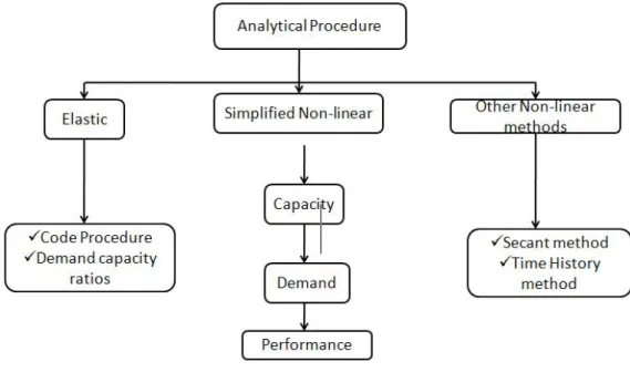
4 REVIEW ON NON-LINEAR METHODS OF ANALYSIS ...30
4.1 Introduction...30
4.1.1 Previous Study on Non-Linear Analysis ... 30
4.1.2 Nonlinear static pushover analysis ... 31
v
4.1.7 Demand... 37
4.1.8 Performance ... 38
4.1.9 Equal displacement rule ... 40
4.1.10 Equal Energy Rule ... 41
4.2 Procedure for seismic analysis of RC Building as per IS 1893 (Part 1): 2002 ...41
4.2.1 Equivalent static lateral force method ... 41
4.2.2 Response Spectrum Method ... 42
4.3 Displacement Coefficient Method (FEMA-273)...44
4.4 Selection of appropriate method of analysis for the study ...46
5 ANALYSIS AND INTERPRETATION OF RESULTS:...47
5.1 Distribution of Lateral Force ...47
5.2 Natural Structural Period of the Structure ... 49
5.3 Ductility reduction factor (Rμ) ...50
5.4 Overstrength factor (Ω) ...55
5.5 Response reduction factor (R)...57
5.6 Re-detailing the model ...68
5.7 Average R-value on different structural conditions ...71
6 CONCLUSION AND RECOMMENDATION... 72
6.1 Conclusions...72
6.2 Limitations of the Study ...73
6.3 Recommendations ... 73
vii
FIGURE 1.1. SEISMIC HAZARD MAP OF NEPAL AND EASTERN HIMALAYAN ...2
FIGURE 1.2. TREND OF BUILDING CONSTRUCTION IN KATHMANDU ...3
FIGURE 2.1 ANALYTICAL PROCEDURES FOR NON-LINEAR ANALYSIS...7
FIGURE 2.2 FLOW CHART OF RESEARCH METHODOLOGY... ...9
FIGURE 3.1. CONCEPT OF RESPONSE REDUCTION FACTOR ...11
FIGURE 3.2. FORCE DISPLACEMENT RELATIONSHIP FOR OVERSTRENGTH ...14
FIGURE 3.3. STIFFNESS VS STRENGTH RELATIONSHIP1 ...16
FIGURE 3.4. STIFFNESS VS STRENGTH RELATIONSHIP2 ...17
FIGURE 3.5. REPRESENTATION OF DISPLACEMENT DUCTILITY . ...18
FIGURE 4.1. COMPONENT FORCE-DEFORMATION CURVE ...34
FIGURE 4.2. GLOBAL CAPACITY (PUSHOVER CURVE) OF A STRUCTURE. ...35
FIGURE 4.3. BI-LINEAR IDEALIZATION OF A GENERIC CAPACITY CURVE...37
FIGURE 4.4. PERFORMANCE POINT IN A STRUCTURE ...38
FIGURE 4.5. RANGES OF PUSHOVER CURVE ...39
FIGURE 4.6. ELASTO-PLASTIC RESPONSE OF STRUCTURE...40
FIGURE 4.7. CONCEPT OF EQUAL ENERGY RULE ...41
FIGURE 4.8. BILINEAR IDEALIZATION OF PUSHOVER CURVE. ...46
FIGURE 5.1. DISTRIBUTION OF LATERAL FORCE...47
FIGURE 5.2. REPRESENTATION OF DISPLACEMENT DUCTILITY ...50
FIGURE 5.3. REPRESENTATION OF DUCTILITY DEMAND ...51
FIGURE 5.4. CALCULATION OF OVERSTRENGTH FACTOR...55
FIGURE 5.5. REPRESENTATION OF FORCE REDUCTION FACTOR ...57
FIGURE 5.6. DESIGN STRENGTH, OVERSTRENGTH AND RRF...62
FIGURE 5.7. COMPARISON OF R VALUE IN X AND Y DIRECTIONS ...69
FIGURE 5.8. COMPARISON OF R IN EQX LOADING...69
FIGURE 5.9. COMPARISON OF R IN EQY LOADING...69
FIGURE 5.10. COMPARISON OF OVERSTRENGTH FACTOR ...70
FIGURE 5.11. COMPARISON OF DUCTILITY REDUCTION FACTOR...70
FIGURE 5.12. COMPARISON OF DISPLACEMENT DUCTILITY IN EQX...70
FIGURE 5.13. COMPARISON OF DISPLACEMENT DUCTILITY IN EQY ...71
viii
TABLE 3.3: STRENGTH REDUCTION FACTOR FOR RC STRUCTURES...24
TABLE 3.4: REDUCTION FACTOR ACCORDING TO IBC 2003...24
TABLE 3.5: DUCTILITY DISPLACEMENT VALUES...25
TABLE 3.6: RESPONSE REDUCTION FACTOR ACCORDING TO BSLJ ...26
TABLE 3.7: RESPONSE REDUCTION FACTOR R FOR BUILDINGS SYSTEMS ...26
TABLE 3.8: STRUCTURAL PERFORMANCE FACTOR ...27
TABLE 3.9: VALUES FOR MODIFICATION FACTOR C0...45
TABLE 3.10: VALUES FOR C2...46
TABLE 5.1: DISTRIBUTION OF LATERAL FORCES:...47
TABLE 5.2: TIME PERIOD OF THE STUDY BUILDINGS...49
TABLE 5.3: DISPLACEMENT DUCTILITY OF STUDY BUILDINGS...52
TABLE 5.4: COMPARISON OF DISPLACEMENT DUCTILITY ...53
TABLE 5.5: DISPLACEMENT DUCTILITY (DEFAULT HINGE)...54
TABLE 5.6: OVERSTRENGTH FACTOR BASED ON DEFAULT HINGE...56
TABLE 5.7: RESPONSE REDUCTION FACTOR BASED ON USER HINGE...59
TABLE 5.8: RESPONSE REDUCTION FACTOR BASED ON DEFAULT HINGE...60
TABLE 5.9: COMPARISON OF RΜ, Ω AND R OF STUDY BUILDINGS ...61
TABLE 5.10: FINAL R VALUE OF STUDY BUILDINGS ...63
TABLE 5.11: RELATION OF R WITH C/B RATIO AND LOAD PATH...64
TABLE 5.12: RELATION OF R WITH SATISFIED C/B RATIO AND LOAD PATH...64
TABLE 5.13: RELATION OF R WITH C/B RATIO AND LOAD PATH...65
TABLE 5.14: RELATION OF C/B RATIO, Μ, RΜ AND R...65
TABLE 5.15: COMPARISON WITH HIGH RΜ AND LESS Ω ...66
TABLE 5.16: COMPARISON WITH LESS RΜ AND HIGH Ω ...66
TABLE 5.17: PERFORMANCE OF STUDY BUILDINGS ...67
ix
Annex 1.3. Capacity check... 81
Annex 2.1. Results from Static Pushover Analysis ... 86
Annex 2.2. Stages for formation of plastic hinge... 99
Annex 3.1. Sample Calculation of R-Value of Study Building ... 106
Annex 4.1. Modal 5 (when proper detailing) ... 114
ANNEX 5.1 Capacity curve of some sample models...116
x
Q3= Lateral force act on cg of third floor Q4= Lateral force act on cg of fourth floor Q5= Lateral force act on cg of fifth floor GF = Ground floor FF = First floor SF = Second floor TF = Third floor TF = Top floor [K]= Stiffness matrix [M]= Mass matrix
∆e = Elastic displacement ∆u = Ultimate displacement ∆y = Yield displacement
Ah = Design horizontal acceleration spectrum value Ak= Design horizontal acceleration spectrum value
As' = Area of compression steel As = Area of tension steel
ATC = Applied Technology Council b = Width of section
C0= Modification factor to relate spectral displacement
C1= Modification factor to relate expected maximum inelastic displacements to displacements calculated for linear elastic response.
C2= Modification factor to represent the effect of hysteresis shape on the maximum displacement response.
C3= Modification factor to represent increased displacements due to second-order effects.
xi
EQX = Earthquake push on X-direction EQY = Earthquake push on y-direction Es = Modulus of elasticity of steel f = Load vector
fc' = Stress in concrete
FEMA = Federal Emergency Management Agency fr = Modulus of rupture
fy = Yield strength of steel
hi= Height of the floor i, measured from base
I = Building occupancy importance I = Moment of inertia
jd = Distance of compressive forces in the steel and concrete K = Horizontal force factor
k = Neutral axis depth factor
Ke = Effective lateral stiffness of the buildings in direction under consideration. Ki = Elastic lateral stiffness of the building in the direction under consideration. Mcrack = cracking moment
n = Number of storey’s in the building n = number of stories Pk = Modal participation factor
Qi= Design lateral force at floor i.
R= Response reduction factor RR= Redundancy factor
Ω = Overstrength factor
μ = Displacement ductility factor Rμ = Ductility reduction factor Rξ = Damping reduction factor. S = Soil profile coefficient S1 = Site coefficient Sa= Spectral acceleration
xii
Vd= Design base shear.
Vu = Ultimate shear force W = Total gravity load
Wi= Seismic weight of the floor i,
y = Depth of neutral axis
z = Distance of critical section to the point of contraflexure Z = Zone factor
α = Ratio of post yield stiffness to effective elastic stiffness δt = target displacement μd = Displacement ductility demand
μs = Displacement ductility supply φcrack = Curvature before cracking
φy = Curvature at first yield of the tension steel. Ω = Overstrength factor
Ωdefault = Overstrength factor when default hinge was used. Ωuser = Overstrength factor when user defined hinge was used. фik= Mode shape coefficient at floor i in mode k,
T1= Predominant period of the ground motion.
lp = Plastic hinge length φult = Ultimate curvature
θp = Plastic rotation
L= Member lengt
φy= Curvature at yield θy= Rotation at yield
1
INTRODUCTION
1.1
Background of the Study
1.1.1
Seismic Hazard of Nepal and Kathmandu Valley
Nepal and the Himalayan range that forms its northern border with China were formed as a result of the collision of the Indian plate with the Tibetans plate about 50 million years ago. This collision still continuous which results in subduction of Indian plate below the Tibetan plate makes Nepal and the entire Himalayan range seismically active.
Nepal lies in a very high seismic hazard zone. Global seismic hazard map shows Nepal in Zone 4 as possible shaking of MMI IX or above with 10% probability of exceedence in 50 years [46]. Probabilistic seismic hazard mapping of Nepal conducted during building code development in Nepal has shown PGA of 0.36 g in Kathmandu Valley in 500 years return period [49]. In summary, Nepal including Kathmandu valley lies in a very high seismic hazard zone.
Looking at the urbanization of Kathmandu valley now, if similar earthquake as that of 1934 A.D was to occur today, the scenario would be devastating, and the fatalities would be very high. For that earthquake scenario, Japan International Cooperation Agency [46] estimated up to 59000 houses destroyed, 18000 deaths and 59000 seriously injured. Another study carried out in the frame work of the Kathmandu valley Earthquake Risk Management Project [47] estimates a total of 40000 deaths, 95000 injuries and 600000 or more homeless.
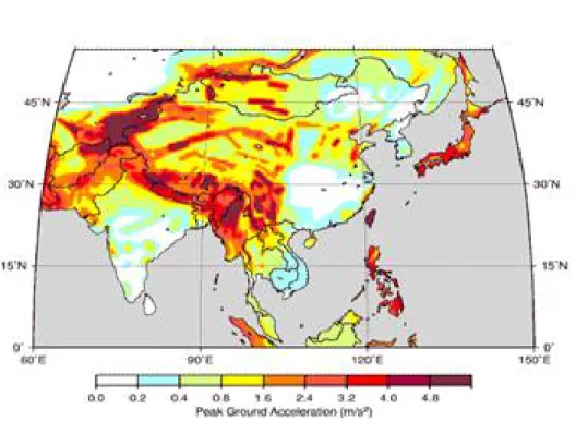
Seismic hazard map of Nepal and Eastern Himalaya (figure 1.1) also gives justify that Kathmandu valley is in highly vulnerable due to earthquake. So, it is urgent need to assess the non-linear behaviour of RC buildings in Kathmandu valley during earthquake.
Figure 1.1. Seismic hazard map of Nepal and Eastern Himalayan
Source: Global Seismic Hazard Assessment Program in Continental Asia (GSHAP). International Lithosphere Program (ILP), 1999
1.1.2
Trend of Building Design and Construction
Most of the casualty from earthquakes is due to collapse of buildings. More than 80 % of the total people killed in developing countries during earthquakes are collapse of buildings.
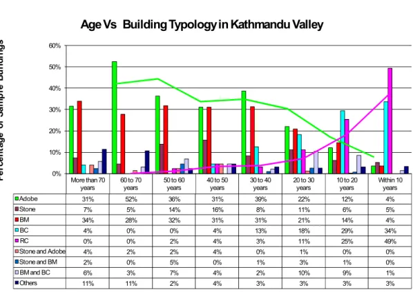
But now-a-days, the trends of RC building construction are rapidly increased [46]. Figure 1.2 shows the trend of building construction in Kathmandu valley and clearly shows that the trends of RC buildings construction is rapidly increasing from the past some years.
Figure 1.2. Trend of Building Construction in Kathmandu Valley
Source: “The Study on Earthquake Disaster Mitigation in the Kathmandu Valley Kingdom of Nepal”. Japan International Cooperation Agency (JICA) and Ministry of Home Affairs, His Majesty‘s Government of Nepal, 2002.
Now-a-days the number of engineer designed buildings is also increasing. The design of RC building mainly based on seismic coefficient method which gives approximate design base shear. The value of Response Reduction Factor (R) = 5 is taken in all the times, considering the building is special moment resisting frame with expectation of very high ductility. To meet these expected very high ductility capacity of structural members has to go very high inelastic deformation. The capacity governs the structural behaviour and damageability of buildings during earthquake ground motions. Sometimes Response spectrum method was also used to determine the design base shear of the structure but it is also far to address the actual base shear which is generated during earthquake.
More than 70
years 60 to 70years 50 to 60years 40 to 50years 30 to 40years 20 to 30years 10 to 20years Within 10years Adobe 31% 52% 36% 31% 39% 22% 12% 4% Stone 7% 5% 14% 16% 8% 11% 6% 5% BM 34% 28% 32% 31% 31% 21% 14% 4%
BC 4% 0% 0% 4% 13% 18% 29% 34%
RC 0% 0% 2% 4% 3% 11% 25% 49%
Stone and Adobe 4% 2% 2% 4% 0% 1% 0% 0% Stone and BM 2% 0% 5% 0% 1% 3% 1% 0% BM and BC 6% 3% 7% 4% 2% 10% 9% 1% Others 11% 11% 2% 4% 3% 3% 3% 3% 0% 10% 20% 30% 40% 50% 60% Pe rc en ta ge o f S am pl e Bu ild in gs Age
governed by the principles of force-based seismic design, there have been significant attempts to incorporate the concepts of deformation- based seismic design and evaluation into earthquake engineering practice. In general, the study of the inelastic seismic response of buildings is not only useful to improve the guidelines and code provisions for minimizing the potential damage of buildings, but also important to provide economical design by making use of the reserved strength of the buildings as it experiences inelastic deformations. In recent seismic guidelines and codes in Europe and USA, the inelastic response of the building are determined using nonlinear static methods of analysis known as the pushover analysis methods but such trends does not established in South Asian region [24].
1.1.3
Research need
Past evidence had shown that the structures in Kathmandu valley are vulnerable due to earthquake [46]. The RC building construction trends increases day by day. Buildings are designed based on linear elastic methods which are considered only elastic range. Assumption was made that Non-linearity of the structure is incorporated by response reduction factor R. The effect of ductility, over strength, load path and column beam capacity ratio on performance of structure is essential to study through non linear analysis.
Table 7 of IS 1893(Part 1): 2002 gives the value of Response Reduction Factor, R, for lateral load resisting system. IS 13920-1993 gives the ductility requirement for earthquake resistant design. For special moment resisting RC frame structures (SMRF) R value is given as 5. While designing the RC structure R value is taken as 5 in all situations. Code does not explain all necessary circumstances of SMRF. Thus it is essential to study the real behaviours of RC buildings in Kathmandu valley through non-linear analysis and suggest the circumstance which affects the response of the structure.
2
OBJECTIVES, APPROACHES AND METHODOLOGIES
2.1
Objective of the Study
The main objective of this research is to verify the designed R factor of most common engineer designed RC buildings in Kathmandu Valley through comparing the assumed R factor during design to actual R factor obtained from non-linear analysis. The specific objectives of the study are to:
Select most common engineer designed RC buildings and study different parameters to consider for analysis
Study different method of non-linear analysis to calculate R factor and select the appropriate method to calculate the R factor
Conduct non-linear analysis and calculate R factor of more than 10 buildings
Compare the calculated R factor with the assumed one and also with different parameters of the building
Evaluate ductility reduction factor of study buildings Evaluate Overstrength factor of study buildings
Check effect of overstrength factor on the ductility factor Check effect of load path on response reduction factor Check beam column capacity ratio on building ductility
Check combined effect of beam column capacity ratio and load path on response reduction factor
2.2
Study Approaches
This study will be a combination of both the field work and desk study for analysis. However, the field work is limited to selection of typical RC buildings for analysis. More work is on desk study as it is more an analytical study.
analysis methods for calculation of R factor is one of the major parts of the study.
2.3
Research Methodology
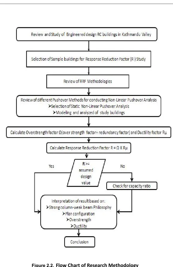
To meet the objectives of the study a methodology has been developed and given in Figure 1.1 below. The research will be started from review and study of RC buildings and lastly conclusions are drawn. The brief description of each steps are:
2.3.1
Review and study of engineered design buildings in Kathmandu
valley
The trends of construction RC buildings, designing criteria, behaviours of structure during earthquake were firstly studied [chapter 1]. The secondary data are used in this study to fulfil the study needs. Apart from this, some primary data are also collected. The sources of secondary data are:
Journal and newspapers
Published and unpublished articles Past studies made in this field
Data from the analysis results from structural analysis program.
2.3.2
Selection of sample building for response reduction factor (R)
study
Sampling was done randomly which represent the nature of deigning trends and construction practices in different localities. The buildings of Kathmandu valley which has Plan less than 2000 sq.ft and up to 5 stories are taken as the population of the study. The site soil condition is taken as medium, clay.
2.3.3
Review of response reduction factor methodologies
Response reduction factor is used to scale down the elastic force of the structure. Elastic force generated during the earthquake is divided by force reduction factor(2R) to obtain design base shear which is used for designing of structure. Ductility factor, over strength factor and redundancy are the key factors for the formulation of response reduction factor. Different methodologies and its formulation is presented in chapter [3]
2.3.4
Review of different pushover methods for conducting non-linear
pushover analysis
Different procedures used for the analysis of non-linear behaviour of the structure were studied and appropriate method for non-linear analysis of study buildings was chosen. The detailed description of the pushover and modeling of structure is given in chapter [4].
After pushover analysis, capacity curve of the structure is obtained. Capacity curve of the structure gives the ultimate deformation and ultimate base shear. Bilinear idealization of capacity curve gives the yield deformation. With the help of these data, over strength factor, displacement ductility, ductility reduction factor and ultimately response reduction factors are calculated. The calculations are based on the mathematical expressions explained in chapter [3] and [4]. Sample calculation of one model is given in Annex 3.1. The final results and interpolation of the results are presented in chapter [5]. Finally, conclusions were drawn based on results which is presented in chapter [6]
3
REVIEW ON CALCULATION METHODOLOGIES FOR RESPONSE
REDUCTION FACTOR
3.1
Definition of Response Reduction Factor
Response reduction is used to scale down the elastic response of the structure [8]. The structure is allowed to be damaged in case of severe shaking. Hence, structure is designed for seismic force much less than what is expected under strong shaking if the structure were to remain linearly elastic.
It is simply represents the ratio of the maximum lateral force, Ve, which would develop in a structure, responding entirely linear elastic under the specified ground motion, to the lateral force, Vd, which has been designed to withstand. Response reduction factor R, is expressed by the equation:
R = Ve/ Vd (1)
The factor R is an empirical response reduction factor intended to account for damping, overstrength, and the ductility inherent in the structural system at displacements great enough to surpass initial yield and approach the ultimate load displacement of the structural system [1]. The concept of a response reduction factor was based on the premise that well-detailed seismic framing systems could sustain large inelastic deformations without collapse(ductile behavior) and develop lateral strength in excess of their design strength(often termed reserve strength)[2]. R factor is first introduced in 1978[3], used to reduce the elastic shear force (Ve) obtained by elastic analysis using a 5% damped acceleration response spectrum for the purpose of calculating a design base shear(Vd). Major static analysis routines are Equivalent Lateral Force Method and Response Spectrum Method; in both procedures R factors are utilized to calculate the design base shear.
Now, the IS code provides the realistic force for elastic structure and divides those forces by (2R) [16].
Figure 3.1. concept of response reduction factor
Source: proposed draft provisions and commentary on Indian Seismic Code IS 1893 -Part 1
3.2
Response Reduction Factor Formulation
In the mid-1980s, Berkeley [1] described R as the product of three factors that accounted for reserve strength, ductility, and added viscous damping
(3) Rs stands for overstrength and calculated to be equal to the maximum base shear force at the yield level (Vy) divided by the design base shear force (Vd).
Rµ stands for ductility factor and calculated as the base shear (Ve) for elastic response divided by the yield base shear (Vy). The damping factor was set equal to 1.0.
ATC 19 [27] splitting R into three component factors.
behavior factors specified in various codes for the same types of structure.
3.3
Previous Studies on calculation of Response Reduction Factors of
Existing Buildings
Tinkoo Kim and Hyunhoo Choi [4]Determine the strength reduction factors for structures with added damping and stiffness device. For the structural period between 0.50 seconds to 5 seconds, the strength reduction factors for TADAS device with ductility equal to 6 varies from 8.30 to 10.70.
Bhavin Patel1and Dhara Shah2[23]
Formulate the key factors for seismic modification factor of RCC framed staging of elevated water tank. The analysis revealed that three major factors, called reserved strength, ductility and redundancy affect the actual value of response modification factor. Conclusion was made that the water tank which is well design by using codal procedure has the response reduction factor 4.0.
Greg Mertz1)and Tom Houston2)[6]
Proposes a methodology to develop force reduction factors that are appropriate for the evaluation nuclear facilities. These force reduction factors are functions of acceptable limit state; the structural system, material, and detailing for each individual element, structure’s natural frequency; and the influence of higher modes and soft stories. The acceptable limit state, structural system, material and detailing is used to develop allowable element ductilities. Individual element ductilities are modified to account for either MDOF or soft story effects. These modified element ductilities are combined with the structures natural frequency and an appropriate SDOF dynamic model to develop the force reduction factor.
A. Kadid and A. Boumrkik [7]
Evaluated the performance of RC framed buildings under future expected earthquakes, a non-linear static pushover analysis has been conducted. To achieve this objective, three frame buildings with 5, 8 and 12 stories were analyzed. The results obtained from this study show that properly designed frames will perform well under seismic loads.
Devrim Ozhendekci, Nuri Ozhendekci and A. Zafer Ozturk [5]
Evaluate the seismic response modification factor for eccentrically braced frames. Conclusion was made that one constant R-value cannot reflect the expected inelastic behavior of all building which have the same lateral load resisting system. In the analysis they used overstrength factor, ductility factor and redundancy factor for the evaluation of R-values to the EBF systems.
R = RΩ* Rμ* RR (5)
3.4
Overstrength Factor
3.4.1
Overstrength
The structure has finally reached its strength and deformation capacity. The additional strength beyond the design strength is called the overstrength. Most structures display considerable overstrength. Sequential yielding of critical regions, material overstrength, strain hardening, capacity reduction factors are the sources of overstrength (Ω).
Overstrength can be employed to reduce the forces used in the design, hence leading to more economical structures. The main sources of overstrength are [13]:
The difference between the actual and design material strength Conservation of the design procedure and ductility requirements Load factors and multiple load cases
Effect of structural elements not considered in predicting the lateral load capacity
Minimum reinforcement and member sizes that exceed the design requirements
Redundancy
Actual confinement effects
Utilizing the elastic period to obtain the design forces.
Member size or reinforcement lager than required, strain hardening in materials, Confinement of concrete, strength contribution of non-structural elements and special ductile detailing are also the sources of overstrength [24]
Overstrength factor (Ω) = apparent strength/design strength [9]
Ω = Vu/Vd (6)
Figure 3.2. Force Displacement relationship for overstrength
3.4.2
Previous Studies on calculation of Overstrength factor of
Existing Buildings
In this section, some of the previous studies about overstrength factor are reviewed
Freeman [10]
The author reported overstrength factors for 3 three storey moment resisting frames, two constructed in seismic zone 4 and one in seismic zone 3 were 1.9, 3.6, and 3.3 respectively.
Kappos [11]
In this study five R/C buildings, with one to five stories, consisting of beam, columns, and structural walls are examined and as a result overstrength factors 1.5 to 2.7 are obtained.
Lee, Cho and Ko [12]
In their study the authors investigated overstrength factors and plastic rotation demands for 5, 10, 15 storey R/C buildings designed in low and high seismic regions utilizing three dimensional pushover analysis. One of their conclusions is that the overstrength factors in low seismicity regions are larger than those of high seismicity regions for structures designed with the same response modification factor. They have reported factors ranging from 2.3 to 2.8.
A.S Elnashai1and A. M. Mwafy2[13]
Develops the relationship between the lateral capacity, design force reduction factor, the ductility level and the overstrength factor. The lateral capacity and overstrength factor are estimated by means of inelastic static pushover as well as time- history analysis of 12 buildings of various characteristics representing a wide range of contemporary RC buildings. Conclusion was made that the recommendations of FEMA 273[14] and Paulay and Priestley [15] underestimate the inelastic period.
3.5.1
Terms used in ductility reduction factors
Strength, stiffness and ductility are the essential structural properties for the seismic protection.
Stiffness
If the deformation under the action of lateral forces is to be reliably quantified and subsequently controlled, designer must make a realistic estimate of the relevant property stiffness. This quantity relates loads or forces to the ensuing structural deformations. A typical non-linear relationship between induced forces or loads and displacements, describing the response of a reinforced concrete component subjected to monotonically increasing displacement. For design computations, one of the two bilinear approximations may be use where Vy defines
the yield or ideal strength Vi of the member [16]. The slope of the idealized linear
elastic response
K = Vy/ ∆y (7)
Figure 3.3 is used to quantify the stiffness.
Figure 3.3. Stiffness Vs Strength relationship1
Structure A has higher strength and lower stiffness as compared to structure B.
Strength
If the structure is to be protected against damage a selected or specified seismic event, inelastic excursions during its dynamic response should be prevented.
This means that the structure must have adequate strength to resist internal actions generated during the elastic dynamic response of the structure [16].
Figure 3.4. Stiffness Vs Strength relationship2
Structure A has higher strength and higher stiffness as compared to structure B.
Ductility
Ductility of a structure, or its members, is the capacity to undergo large inelastic deformations without significant loss of strength or stiffness. Ductility is a very important property, especially when the structure is subjected to seismic loads. Ductile structures have been found to perform much better in comparison to brittle structures [16]. High ductility allows a structure to undergo large deformations before it collapse. Large structural ductility allows the structural to move as a mechanism under its maximum potential strength, resulting in the dissipation of large amount of energy [1].
The extent of inelastic deformation experienced by the structural system subjected to a given ground motion or a lateral loading is given by the displacement ductility ratio “µ” and it is represented by the ratio of maximum absolute displacement to its yield displacement [9].
The inelastic behavior of structure can be idealized as [9]
μ = ∆u / ∆y (7)
Where μ∆is the displacement ductility, ∆u is the ultimate deformation and ∆y is the
Figure 3.5. Representation of displacement ductility (source FEMA 451).
Yield deformation is obtained as follows [17]
The nonlinear force-displacement relationship between base shear and displacement of the control node shall be replaced with an idealized relationship to calculate the effective lateral stiffness, Ke, and effective yield strength Vby, of the structure shown in figure 4.8. The relation shall be bilinear, with initial slope Ke and post-yield slope γ. line segments on the idealized force-displacement curve shall be located using an iterative graphical procedure that approximately balances the area below and above the curve. The effective lateral stiffness, Ke, shall be taken as the secant stiffness calculated at a base shear force equal to 60% of the effective yield strength of the structure. Thus, Vy is the intersection of initial and effective stiffness.
3.5.2
Previous studies on Calculation of Ductility Reduction Factors of
Existing Buildings
Newmark and Hall [18]
Define the ductility factor is the ratio of maximum deformation to the yield deformation and proposed the following equations for the determination of ductility reduction factor (Rμ).
Rμ= 1.0 (T < 0.03 second) (8a)
Rμ= 2μ − 1 (0.12 < T < 0.03 second) (9a)
Rμ= μ (T > 1.0 second) (10a)
T. Paulay and M. J. N. Priestley [48]
Divides the time period of the structure for calculating ductility reduction factor.
Rμ= 1.0 for zero-period structures (8a)
Rμ= 2μ − 1 for short-period structure (9a)
Rμ= μ for long period structure (10a)
Rμ= 1+ (μ-1) T/0.70 (0.70 s < T < 0.3) (11)
Miranda and Bertero [19]
Introduced the equation for reduction factor by considering 124 ground motions recorded on a wide range of soil conditions. The soil conditions were classified as rock, alluvium and very soft sites characterized by low shear wave velocity. A 5% of critical damping was assumed. The ductility factor was give by
Rμ=μф +1 (12)
Values of are calculated by using the relations:
ф = 1+ μ - exp (-2(ln (T)-0.2)2) for alluvium site (13)
Lai and Biggs [20]
In this study design inelastic response spectra were based on mean inelastic spectra computed for 20 artificial ground motions. Analyses carried on for periods equally spaced between 0.1s and 10s with 50 natural periods. The ductility reduction factors corresponding to the proposed coefficients are given by
Table 3.1: α & β coefficients proposed by authors Lai & Biggs
M. Mahmoudi [21]
Develops the relationship between overstrength and member ductility of RC moment resisting frames having one, two, three, four, five, six, eight, ten and fifteen stories with three spans. The results indicate that the overstrength depends on member ductility considerably and its amount is not equal for structures having low, medium and high ductility.
Ioana Olteanu, Ioan-Petru Clongradi, Mihaela Anechitei and M. Budescu[22]
Presents the characteristics of the ductility concept for the structural system. The reduction of the seismic forces is realized based on the ductility, redundancy and the strength excess of the structure. Among these, the most significant reduction of the design forces is based on the ductility of the structure that depends on the chosen structural type and material characteristics.
3.5.3
Ductility of unconfined beam sections.
Calculation of moment and curvature [25].a) At just prior to cracking of the concrete b) At first yield of the tension steel.
c) When the concrete reaches an extreme fibre strain of 0.004 a) Before cracking (elastic behaviors)
Mcrack= fr *I/ ybottom (15)
.
φcrack= / (16)
b) At first yield of the tension steel
My= As fyjd (17)
k = [(ρ+ρ')2n2+2(ρ+ρ'd'/d) n ]1/2– (ρ+ρ') n (18)
φy = /( ) (19)
a = (As fy - As' fy)/ 0.85 fc' b (20)
Mu = 0.85 fc' a b (d-a/2) + As' fy (d-d') (21)
c) When the concrete reaches the extreme fibre strain
φu= εc/ c (22)
n = Es / Ec (23)
ρ = As/ bd (24)
ρ' = As'/ bd (25)
The same concept is followed by SAP 2000 [33] to develop moment curvature relation.
Plastic hinge length
Various empirical expressions have been proposed by investigators for the equivalent length of plastic hinge lpand the maximum concrete strain εcat ultimate
curvature. BAKER:
b) for members confined by transverse steel
lp= 0.80 k1k3( z/d) c (27)
CORLEY:
For simply supported beam
lp= 0.50 d + 0.20 √ (z/d) ; εc= 0.003 +0.02 b/z + (ρsfy/2 (28) Mattok suggested lp= 0.50 d+ .05d (29) εc= 0.003+0.02 b/z +0.20 ρs (30) Sawyer: lp= (0.25d+0.075z) Where,
k1= 0.70 for mild steel or 0.90 for cold worked steel.
K2 = 1+ 0.50 Pu/Po, where Pu = axial compressive force in member and Po is axial
compressive strength of member without bending moment.
K3 = 0.60 when fc' = 35.2 N/mm2or 0.90 when fc' =11.7 N/mm2; assuming fc' = 0.85 * cube strength of concrete.
z = distance of critical section to the point of contraflexure d = effective depth of member.
A good estimate of the effective plastic hinge length may be obtained from the expression.
lp= 0.08 l+ 0.022 dbfy
Where
db= nominal diameter of bar in mm.
For user-defined hinge properties, the procedure used by Park and Paulay [25] is used to determine moment –rotation relationships of members from the moment-curvature relationships. In this procedure, the moment is assumed to vary linearly along the beam and columns with a contraflexure point at the middle of the members. With this assumption, the relations are
Plastic hinge rotation capacity of members is estimated using the following equations proposed by ATC-40 [26] and value at ultimate moment is obtained by adding plastic rotations to the yield rotation.
θp = (φult – φy) lp (32)
ATC-40[26] suggests that plastic hinge length equals to half of the section depth in the direction of loading. This technique was adapted to calculate plastic hinge length in this study.
3.6
Redundancy Factor
Redundant is usually defined as: exceeding what is necessary or naturally excessive. Building should have a high degree of redundancy for lateral load resistance [16]. More redundancy in the structure leads to increased level of energy dissipation and more overstrength. In a nonredundant system the failure of a member is equivalent to the failure of the entire structure however in a redundant system failure will occur if more than one member fails. Thus, the reliability of a system will be a function of the system’s redundancy meaning that the reliability depends on whether the system is redundant or nonredundant[16].
Table 3.2: Redundancy factor (RR) was taken from ATC
Lines of vertical seismic framing Drift redundancy factor
2 0.71
3 0.86
4 1.0
Overstrength, redundancy and ductility together contribute to the fact that an earthquake resistant structure can be designed for much lower force than is implied by the strong shaking.
In design codes the considered seismic force used to dimensioning the structural elements is multiplied by several coefficients, in order to simplify the design process. One of them is the reduction factor. The behavior factor of the response is computed as a product of three factors
R = RsRμRξ,
3.7.1
Response Reduction Factor as per ATC-19
In the ATC-19[27] meeting from 1995 damping reduction factor was replaced by the redundancy factor RR. R = (RsRμ) RR
Table 3.3: The strength reduction factor for Reinforced Concrete Structures
Structural type Rs
Rc structures medium and high elevation 1.6……….4.6
Rc structures with irregularities in elevation 2.0………..3.0
3.7.2
Response Reduction Factor as per IBC, 2003
The seismic force at the bottom of the building, according to the American design code, is computed with the following relationship (IBC, 2003) [28]:
V = . W
Table 3.4: Reduction factor According to IBC 2003
Structural type R
Special Rc frames 8.0
Intermediate Rc frames 5.0
3.7.3
Response Reduction Factor as per New Zeeland design norm
According to the New Zeeland design norm[30], the coefficient Cμfrom theseismic force relation is determined by taking into consideration the fundamental oscillation period, T1, the ductility displacement, μ∆, and soil type,
Ftot= CμR Z Wt
The value of Cμ coefficient ranges between 0.40 and 0.040, for ductile Rc structures with the ductility displacement, μ, between 4 and 6. The values of the ductility displacement, μ∆, are listed in table
Table 3.5: Ductility displacement values, μ∆, according to New Zeeland design norms
Structures RC Prestressed concrete
Structures with elastic behaviors 1.25 1.00
Structures with limited ductility -
-Frames 3.00 2.00
Coupled walls 2.00
-Ductile structures -
-Moment resisting frames 6.00 5.00
Walls 5.00
-3.7.4
Response Reduction Factor in Japanese design code
According to Japanese design code [30] the seismic force at the bottom of the structure is computed using the following relation (Building standard Law of Japan, 2004)
Vun,i= Ds,iFes,iVi.
The coefficient Ds,i depends on the structural type and it represents the inverted value of the behaviour factor from the European norm. This factor is influenced by
structures depending on the structural type and ductility class.
Table 3.6: Response Reduction Factor According to BSL J
Ductility Moment-resisting frame Other frames Frames with bracing
Excellent 0.30 0.35 0.40
Good 0.35 0.40 0.45
Normal 0.40 0.45 0.50
Low 0.45 0.50 0.55
3.7.5
Response Reduction Factor in IS 1893 (part1):2002
According to IS 1893[16] (part1):2002, Criteria for Earthquake Resistant Design of Structures, design seismic base shear can be computed as
VB= AhW
Ah=
Where, R is the response reduction factor, depending on the perceived seismic damage performance of the structure, characterized by ductile or brittle deformations. The values of R of the buildings are given in the table.
Table 3.7: Response reduction factor R for Buildings Systems
Lateral load resisting system R
Building frame system
Ordinary RC moment-resisting frame (OMRF) 3.0
Special RC moment-resisting frame ( SMRF) 5.0
3.7.6
Response Reduction Factor in NBC 105:1994
Nepal National Building Code, NBC 105:1994 [32], establish the following relation for Seismic Design of Buildings in Nepal.
The design horizontal seismic force coefficient, Cd shall be taken as Cd = CZIK
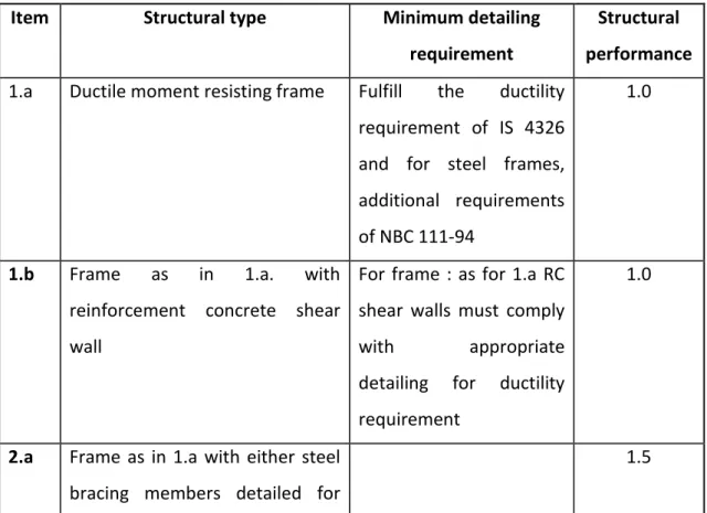
Where, K is the structural performance factor. The structural type may be different in each of two directions in a building and in that case the appropriate value for K shall be selected for each direction. When more than one structural type is used in the structure for the direction under consideration, the structural performance factor for the element providing the majority of the seismic load resistance shall be applied provided that the elements of the other structural types have the ability to accept the resulting deformations.
Table 3.8: Structural performance factor Item Structural type Minimum detailing
requirement
Structural performance 1.a Ductile moment resisting frame Fulfill the ductility
requirement of IS 4326 and for steel frames, additional requirements of NBC 111-94
1.0
1.b Frame as in 1.a. with
reinforcement concrete shear wall
For frame : as for 1.a RC shear walls must comply
with appropriate
detailing for ductility requirement
1.0
2.a Frame as in 1.a with either steel bracing members detailed for
infill panels
2.b Frame as in 1.a with masonry infill
Must comply with
detailing requirements of : IS 4326
2.0
3 Diagonally- braced steel frame with ductile bracing acting in tension only
Must comply with the detailing for ductility requirements of Nepal Steel Construction Standard
2.0
4. Cable –stayed chimneys Appropriate materials
standard
3.0
5. Structures of minimal ductility including reinforced concrete frames not covered by 1 or 2 above, and masonry bearing wall structures
Appropriate materials standard
4.0
Building codes allow for an elastic structural analysis based on applied forces reduced accounting for the presumed ductility supplied by the structure. For elastic analysis, use of reduced forces will result in a significant underestimate of displacement demands. Therefore, the displacements from the reduced-force elastic analysis must be multiplied by the ductility factor to produce the true “inelastic” displacements.
3.8
Formulation used for this study
For the determination of Overstrength factor (Ω) concept of FEMA 451 is used, which gives
Ω = Vu / Vy Χ Vy/Vd = Ωo Χ RR
Ω = Vu/Vd (6)
The expression of equation (6) is same as the indication given by IS 1893-2002. For the determination of displacement ductility following expression is used
μ= ∆u / ∆y (7)
For determination of ductility reduction factor, equation (11) is used Rμ= 1+ (μ-1) T/0.70 (0.70 s < T < 0.3)
For the determination of Response Reduction Factor (R), the main concept given by
ATC-19 is used, which is given in equation (4)
R = Ω × Rμ × RR
But in our case, Overstrength and redundancy factor is taken as single term i.e overstrength factor and the IS 1893-2002 gives the value of Force Reduction Factor = (2R), same concept is used to determine Response Reduction Factor of the study structures.
2R = Ω × Rμ R = Ω × Rμ/2
4
REVIEW ON NON-LINEAR METHODS OF ANALYSIS
4.1
Introduction
Researcher formulates the different techniques for the study of non-linear behaviors of the structure.
4.1.1
Previous Study on Non-Linear Analysis
Krawinkler H. and Seneviratha [39]Conducted a detailed study on pushover analysis. The accuracy of pushover predictions were evaluated on a 4-story steel perimeter framed in 1994 Northridge earthquake. The comparison of pushover and nonlinear dynamic analysis results showed that pushover analysis provides good predictions of seismic demands for low-rise structures having uniform distribution of inelastic behavior over the height.
Mwafy A.M. and Elnashai [40]
Performed a series of pushover analysis and incremental dynamic collapse analysis to investigate and the applicability of pushover analysis. Twelve RC buildings with different structural system were studied. The results showed that triangular load pattern outcomes were in good correlation with dynamic analysis results. It was also noted that pushover analysis is more appropriate for low-rise and short period structures and triangular loading is adequate to predict the response of such structures.
Chopra A.K and Goel R.K [41]
Developed an improved pushover analysis procedure named as Modal Pushover Analysis (MPA) which is based on structural dynamic theory. Firstly, the procedure was applied on to linearly elastic buildings and it was shown that the procedure is equivalent to the well known response spectrum analysis. Then, the
procedure was extended to estimate the seismic demands of inelastic systems. The MPA was more accurate than all pushover analysis is estimating floor displacements, storey drifts, plastic hinge rotations and plastic hinge locations.
4.1.2
Nonlinear static pushover analysis
It is the incremental analysis used by SAP 2000. It divides the load applied and the target displacement to the predefined nos of steps. Each steps of load will be applied to the structure. The steps is increased or decreased so that the target incremental displacement is achieved. The target incremental displacement and corresponding sum of lateral forces is recorded. The stress and deformation output from previous step will be imposed to next step of loading. The process is repeated till the instability of structure or target displacement.
Virote Boonyapinyo1, Norathape Choopool2and Pennung Warnitchai3.[42]
The performances of reinforced-concrete buildings evaluated by nonlinear static pushover analysis and nonlinear time history analysis were compared. The results show that the nonlinear static pushover analysis is accurate enough for practical applications in seismic performance evaluation when compared with nonlinear dynamic analysis of MDOF system.
A.Kadid and A. Boumrkik. [43]
Use a non linear pushover analysis to evaluate the performance of framed buildings under expected earthquakes in Algeria. The results obtained from this study show that properly designed frames will perform well under seismic loads.
Gergely, P., R.N. White, and K.M. Mosalam, [44]
Use static nonlinear pushover analysis for evaluation and modeling of infilled frames buildings. Conclusions are made that elastic seismic analysis methods are inadequate for the estimation of the internal force and displacement distributions.
Pushover analysis can be performed as either force-controlled or displacement- controlled depending on the physical nature of the load and the behavior expected from the structure. Force-controlled option is useful when the load is known (such as gravity loading where structure is loaded gravity load plus 25 % of live load) and the structure is expected to be able to support the load. Displacement- controlled procedure is used when specified drifts are sought (such as in seismic loading), where the magnitude of the applied load is not known in advance, or when the structure can be expected to lose strength or become unstable. The first mode response of the structure was assigned as the load pattern for the lateral push applied to the structure.
Nonlinear version of finite element package SAP2000 [33] can model nonlinear behavior and perform pushover analysis directly to obtain capacity curve for three dimensional models of the structure. A displacement-controlled pushover analysis is basically composed of the following steps:
Developing a three dimensional bare frame model of existing RC buildings. Application of gravity loads and live loads.
Application of 10% static lateral load induced due to earthquake, at CG of the building
Developing M-θ relationship for critical regions (Plastic hinging zone) of beam and column element with shear strength confirming and non confirming. Pushing the structure using the load patterns of static lateral loads, up to
displacements larger than those associated with target displacement using static pushover analysis
Developing hinge progressing sequence in different steps of the loading. Developing tables of roof displacement vs. base shear or pushover curve.
The earthquake forces are estimate as per IS 1893-2002 (part-2) [16]. Moment – rotation and Axial load- Bending moment (P-M2-M3) relationships for flexural and compression members have been developed using SAP 2000 software. Above relationships are also analytically calculated by the methods suggested by R. Park and T. Paulay [25].
4.1.4
Default Vs User-Defined Hinge Properties for Concrete Sections
The built-in default hinge characteristics of concrete sections are based on ATC-40[26] and FEMA-273[14] criteria which consider basic parameters controlling the behavior. Based on these parameters, in this study, default moment hinges assigned to all beams have same plastic rotation capacities (M3) and default PMM hinges assigned to all columns have same plastic rotation capacities regardless of the section dimensions. Slope between points B and C is taken as 10% total strain hardening for steel and yield rotation is taken as zero for default concrete moment and PMM hinges and then user defined hinge properties is assign to the elements.For user-defined hinge properties, the procedure used by Park and Paulay [25] was utilized to determine moment-rotation relationships of members from the Moment-curvature relationships. In this procedure, the moment is assumed to vary linearly along the beams and columns with a contra- flexure point at the middle of the members. Based on this assumption, the relationship between curvature and rotation at yield is obtained.
In this study user defined plastic hinge is generated only on beam element. In Numerical model, there is only option to put the reinforcement of column element. Moment curvature relation of beam element according to the detailing of beam section is established which gives ultimate moment, yield moment, ultimate curvature, yield curvature. Plastic hinge length is taken as 0.50 d (ATC-40). From these data, scale factor, rotation of various segments of plastic hinge is obtained. (Detail in annex)
properties and the effect of hinge properties were illustrated on pushover curves as shown in figure.
Pushover analyses with default and user-defined hinge properties yield differences in sequence of plastic hinging and hinge pattern. The rotation value at the yield point of hinges is not needed for pushover analyses performed by SAP2000 because the program uses cross-sectional dimensions in the elastic range.
Default hinge properties based on ATC-40[26] and FEMA-273[14] criteria are generally preferred to perform pushover analysis by SAP2000 because determination of cross-sectional characteristics of all members of a structure, especially for a three dimensional structure, and inputting these sectional properties into the program make the pushover analysis impractical. Thus, the results of a pushover analysis with default hinge properties should be interpreted with caution since default hinges could not simulate the exact nonlinear behavior of the structure.
4.1.5
Force-Displacement Relationships
When the structure is analyzed with three loading conditions (GRAV, EQX and EQY), pushover curve of the structure is obtained. The curve is the base shear vs. deformation curve.
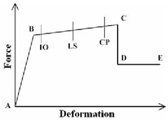
Figure 4.1. Component Force-Deformation Curve
A generic component behavior curve is represented in figurer. The points marked on the curve are expressed by the software vender [33] as follows:
Point A is the origin
Point B represents yielding. No deformation occurs in the hinge up to point B, regardless of the deformation value specified for point B, the deformation (rotation) at point B will be subtracted from the deformations at points C, D, and E. Only the plastic deformation beyond point B will be exhibited by the hinge.
Point C represents the ultimate capacity for pushover analysis. However, a positive slope from C to D may be specified for other purposes.
Point D represents a residual strength for pushover analysis. However, a positive slope from C to D or D to E may be specified for other purposes. Point E represents total failure. Beyond point E on the horizontal axis, if it is
not desired that the hinge to fail this way, a large value for the deformation at point D may be specified.
4.1.6
Capacity
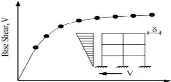
Capacity is a representation of the structures ability to resist the seismic demand. The overall capacity of a structure depends on the strength and deformation capacities of the individual components of the structure [36]. In order to determine the capacities beyond the elastic limit, non linear analysis is required.
Figure 4.2. Global capacity (Pushover curve) of a structure.
Capacity curve is the fundamental for the determination of response reduction factor.
force, initial stiffness and effective stiffness can be obtained from the capacity curve. The health of the structure is judged by the capacity curve.
Idealization of Capacity Curve
The capacity curve presents the primary data for the evaluation of the response reduction factor for structures, but first of all it must be idealized in order to extract the relevant information from the plot. The intension is to obtain the overstrength and the ductility reduction factor by studying the pushover curve.
For this purpose a bi-linear curve is fitted to the capacity curve, such as the first segment starts from the origin, intersects with the second segment at the significant yield point and the second segment starting from the intersection ends at the ultimate point. The slope of the first segment is found by tracing the individual changes in slopes of the plot increments; the mean slope of the all increments are calculated from each step and compared with the latter, searching for a dramatic change. First segment, referred to as elastic portion, is then obtained with a mean slope of the successive parts of the curve until a remarkable change occurs. The second segment, referred to as post-elastic portion, is plotted by acquiring the significant yield point by means of equal energy concept in which the area under the capacity curve and the area under the bi-linear curve is kept equal. Graphical method or auto cad program is developed to read and plot the pushover data then fit the bi-linear curve by utilizing the above mentioned methodology.
This method is an improved version of the one, proposed by FEMA 273[14] which offers a visual trial & error process and suggests that the first segment intersects the original curve at 60% of the significant yield strength.
Figure 4.3. Bi-linear Idealization of a Generic Capacity Curve
Bi-linear idealization provides the essential components, which are significant strength and the significant yield displacement as well as the predetermined design strength and the ultimate displacement. With the help of these data, the overstrength factor which is calculated as the ratio of the yield strength to the design strength. Moreover, ductility ratio can be calculated as the ratio of maximum displacement to the yield displacement which is the key element in calculation of the ductility reduction factor.
4.1.7
Demand
Demand is the representation of the earthquake induced ground by ground motion. Ground motions during an earthquake produce complex horizontal displacement patterns in the structures that may vary with time [36]. For a given structure and ground motion, the displacement demand is an estimate of the maximum expected response of the building during the ground motion.
Procedure to determine demand [ATC-40]
1. Construct a bilinear representation of the capacity curve.
Draw the post-elastic stiffness Ks by judgment to represent an average
through the point on the capacity curve corresponding to a base shear of 0.60Vy, where Vyis defined by the intersection of the Keand Ks.
2. Calculate effective fundamental period.
3. Calculate the target displacement by displacement coefficient method.
Alternately, the displacement demand during earthquake is obtained by considering FEMA 451. Geometrically, the ratio of Ve /Vy is numerically equal to the ratio of ∆u/∆y. so in this study for the calculation of ductility supply the ratio of ∆u/∆y is used. For the prediction of ductility demand, total elastic force is calculated without considering reduction factor. Stiffness of the structure is determined by using K = Ve/∆e (FEMA 356).
For example, modal 3 have the design base shear 379.6 KN (calculation is based on IS 1893-2002). If force reduction factor is not considered, the total elastic force demand is 3796, which is 10 times more than design force.
From capacity curve, the initial stiffness of the structure is 46402 KN/m, then displacement ductility demand is calculated as (µd) =Ve/K, where Ve is the elastic base shear demand and K is the initial stiffness which represent the slope when the structure is in fully elastic.
Thus, µd = 3796/46402 =0.082 m
4.1.8
Performance
The performance is dependent on the manner that the capacity is able to handle the demand [29].
The NEHRP Guidelines for Seismic Rehabilitation of Buildings, FEMA 273 and Provision for seismic Regulations for New buildings and other structures, FEMA 302 define three discrete Structural Performance Levels namely Immediate Occupancy Level (IO), Life Safety (LS), and Collapse Prevention (CP)
Immediate Occupancy (IO)
It is the post earthquake damage state where only minor structural damage has occurred with no substantial reduction in building strength. So, the building is safe to occupy but possibly not useful until repaired.
Life Safety (LS)
It is the post earthquake damage state in which significant damage to the structure has occurred, but some margin against the partial or total collapse remain. In this stage, the building is safe during the earthquake but probably
Collapse Prevention (CP)
It is the post earthquake damage state in which the structure is on the verge of experiencing either local or total collapse.
Figure 4.5. Ranges of pushover curve (Source: ELSEVIER, ENGINEERING STRUCTURE JORUNAL)
Figure 4.6. Elasto-Plastic Response of Structure
In figure [4.6], “The relationship between elastic displacement B and inelastic displacement E depends on the natural period of the structure. If the period is greater than 0.7 s, analyses have shown that E is approximately equal to B (i.e., the deflection of the equivalent elastic structure is approximately equal to that of the elasto-plastic structure, ∆u = ∆e). This is referred to as the Equal Displacement
Principle” [45].
Structure which have time period greater than 0.7 s, ductility reduction factor is calculated by using the equation:
Rμ = μ (T > 0.70 s) ………. (33)
4.1.10
Equal Energy Rule
Low period structure tends to display significant residual deformations. So, in low period structure equal energy concept is used. [9]
Deformation
Figure 4.7. Concept of Equal Energy Rule FE/FI= Rμ = 2μ − 1 (T < 0.3 s) [48]...34
NBC [45], indicates that for period less than 0.3 s, analyses have shown that Equal Energy Principal applies. That is, the area OAB is equal to OCDE [figure 4.6].
A gradual variation in R is found to occur between structural period of 0.3 s and 0.7s.
Rμ = 1+ (μ-1) T/0.70[48]...35
Equation 33 is consistent with assuming that the deflection of the elastic and elasto-plastic systems is the same [49].
Equation (34) is consistent with assuming that the potential energy stored at the maximum deflection is same for the elastic and elasto-plastic systems [49].
4.2
Procedure for seismic analysis of RC Building as per IS 1893 (Part
1): 2002
4.2.1
Equivalent static lateral force method
Total design lateral force or design seismic base shear Vbalong any principal
direction shall be determined by Vb= AhW
Determination of Design Base Shear Design base shear, VB= AhW
Ah= Z/2*I/R*Sa/g
Qi= Vb. ∑
4.2.2
Response Spectrum Method
Procedure for calculating design base shear without considering the stiffness of infill.
a) Determination of Eigen values and Eigenvectors
Mass matrices and stiffness matrices of the frame lumped mass model are, M = [M] and K = [K]
For the above stiffness and mass matrices, eigenvalues and eigenvectors are worked out as follows
|K-ω2m|= 0
By solving the above equation, natural frequencies (eigenvalues) of various modes are calculated. The quantity of ωi2, is called the ith eigenvalue of a matrix [-M ωi2+K]
фi. Each natural frequency (ωi) of the system has a corresponding eigenvector (mode
shape), which is denoted by фi. The mode shape corresponding to each natural frequency is determined from the equations
[-M ωi2+K]ф1=0
[-M ωi2+K]ф2=0
[-M ωi2+K]ф3=0
[-M ωi2+K]фn=0
Solving the above equation, modal vector (eigenvectors), mode shape and natural period under different modes are found
{ф} = {ф1ф2ф3ф4…………..фn}
Determination of Modal Participation Factors The modal participation factor (Pk) of mode k is,
Determination of Modal Mass
Determination of Lateral Force at Each Floor in Each Mode The design lateral force (Qik) at floor i in mode k is given by Qik= AkфikPkWi
Determination of Storey Shear Forces in Each Mode The peak force is given by,
Determination of Storey Shear Force due to All Modes can be obtained as;
The peak storey shear force (Vi) in storey i due to all modes considered is
obtained by combining those due to each mode in accordance with modal combination i.e. SRSS (square root if sum of squares) or (complete quadratic combination) methods.
Square roof of sum of squares (SRSS)
If the building does not have closely spaced modes, the peak response quantity (λ) due to all modes considered shall be obtained as,
The base shear to the study buildings is vertically distributed by using equivalent static lateral force method, but response spectrum method is used in one building compare the differences in design base shear.