Research Article
A Machine Learning Approach to Predict Air Quality in California
Mauro Castelli ,
1Fabiana Martins Clemente,
1Aleˇs Popoviˇc,
1,2Sara Silva,
3and Leonardo Vanneschi
1,31NOVA Information Management School (NOVA IMS), Universidade Nova de Lisboa, Campus de Campolide,
Lisboa 1070-312, Portugal
2University of Ljubljana, School of Economics and Business, Kardeljeva Ploˇsˇcad 17, Ljubljana 1000, Slovenia
3LASIGE, Departamento de Inform´atica, Faculdade de Ciˆencias, Universidade de Lisboa, Lisboa 1749-016, Portugal
Correspondence should be addressed to Mauro Castelli; [email protected] Received 25 January 2020; Accepted 23 June 2020; Published 4 August 2020 Guest Editor: Felix Chan
Copyright © 2020 Mauro Castelli et al. This is an open access article distributed under the Creative Commons Attribution License, which permits unrestricted use, distribution, and reproduction in any medium, provided the original work is properly cited. Predicting air quality is a complex task due to the dynamic nature, volatility, and high variability in time and space of pollutants and particulates. At the same time, being able to model, predict, and monitor air quality is becoming more and more relevant, especially in urban areas, due to the observed critical impact of air pollution on citizens’ health and the environment. In this paper, we employ a popular machine learning method, support vector regression (SVR), to forecast pollutant and particulate levels and to predict the air quality index (AQI). Among the various tested alternatives, radial basis function (RBF) was the type of kernel that allowed SVR to obtain the most accurate predictions. Using the whole set of available variables revealed a more successful strategy than selecting features using principal component analysis. The presented results demonstrate that SVR with RBF kernel allows us to accurately predict hourly pollutant concentrations, like carbon monoxide, sulfur dioxide, nitrogen dioxide, ground-level ozone, and particulate matter 2.5, as well as the hourly AQI for the state of California. Classification into six AQI categories defined by the US Environmental Protection Agency was performed with an accuracy of 94.1% on unseen validation data.
1. Introduction
With the economic and technological development of cities, environmental pollution problems are arising, such as water, noise, and air pollution. In particular, air pollution has a direct impact on human health through the exposure of pollutants and particulates, which has increased the interest in air pollution and its impacts among the scientific com-munity [1–3]. The main causes associated with air pollution are the burning of fossil fuels, agriculture, exhaust from factories and industries, residential heating, and natural disasters.
Air quality has been studied for the last three decades in the United States (US) since the creation of the Clean Air Act program. Although this program has entailed an im-provement in air quality over the years, air pollution is still a problem [4]. Total combustion emissions in the US are accountable for about 200,000 premature deaths per year due to the concentration of pollutants such as particulate
matter 2.5 (PM2.5) and 10,000 deaths per year due to ozone
concentration changes. The American Lung Association estimated that air pollution-related illnesses cost approxi-mately 37 billion dollars each year in the US, with California alone hitting $15 billion [5].
In the face of increasingly serious environmental pol-lution problems, scholars have conducted a significant quantity of related research, and in those studies, the forecasting of air pollution has been of paramount impor-tance. Thus, in full knowledge of the increasing pollution derived problems, the importance of accurately forecasting the levels of air pollutants has increased, playing an im-portant role in air quality management and population prevention against pollution hexes.
The study aims to build models for hourly air quality forecasting for the state of California, using one of the most powerful existing machine learning (ML) approaches, namely, a variant of support vector machines (SVMs), called support vector regression (SVR). The proposal is to build an
Volume 2020, Article ID 8049504, 23 pages https://doi.org/10.1155/2020/8049504
SVR model for the prediction of each pollutant and par-ticulate measurement on an hourly basis and an SVR model to predict the hourly air quality index (AQI) for the state of California.
The paper is organized as follows. Section 2 frames and motivates the work, giving an idea of the impactful con-tribution represented by a successful predicting model for air quality. Section 3 contains a critical revision of the literature, discussing previous and related work. In Section 4, we in-troduce SVM, with a particular focus on the functioning of SVR. Section 5 contains a description of the data used in this work. In Section 6, we discuss the data preprocessing phase that we performed to obtain a more compact and infor-mative dataset to be used by SVR. Section 7 presents our experimental study; it is partitioned into a description of the employed experimental settings and a discussion of the obtained results. Finally, Section 8 concludes the paper and discusses ideas for future research.
2. Background and Motivation
Air pollution is considered to occur whenever harmful or excessive quantities of defined substances such as gases, particulates, and biological molecules are introduced into the atmosphere. These excessive emissions have obvious consequences, causing diseases and death of populations and other living organisms and impairing crops. Air pollutants can either be solid particles, liquid droplets, or gases, which are classified into the following:
Primary pollutants, which are emitted from the source directly to the atmosphere. The sources can be either natural processes, such as sandstorms or human-re-lated, such as industry and vehicle emissions. The most common primary pollutants are sulfur dioxide (SO2),
particulate matter (PM), nitrogen dioxide (NOx), and
carbon monoxide (CO).
Secondary pollutants, which are air pollutants formed in the atmosphere, resulting from the chemical or physical interactions between primary pollutants. Photochemical oxidants and secondary particulate matter are the major examples of secondary pollutants. The most common air pollutants are known as the criteria pollutants, which correspond to the most wide-spread health threats, e.g., CO, SO2, lead, ground-level
ozone (O3), NO2, and PM. The levels of these pollutants are
measured by the US Environmental Protection Agency (EPA), which controls overall air quality. Scientific research has demonstrated a correlation between short-term ex-posure to this kind of pollutants and many health prob-lems, like limited ability to respond to increased oxygen demands when exercising (especially for people with heart conditions), airway inflammation in healthy people and increased respiratory symptoms for people with asthma, respiratory emergencies particularly for children and the elderly, and so on [6].
EPA, EU, and many other national environmental agencies have set standards and air quality guidelines re-garding allowable levels for these pollutants. The air quality
index (AQI) is an indicator created to report air quality, measuring how clean or unhealthy the air is and what as-sociated health effects might be a concern, especially for risk groups. It focuses on health effects that can be experienced within a few hours or days after being exposed to polluted air. It is calculated based on the maximum individual AQI registered for the criteria pollutants mentioned above.
Building a forecasting system, based on the levels of concentration of individual pollutants, that can predict air quality hourly, will make the AQI more flexible and useful for the population’s health. Systems that can generate warnings based on air quality are therefore needed and important for the populations. They may play an important role in health alerts when air pollution levels might exceed the specified levels; also, they may integrate existing emis-sion control programs, for instance, by allowing environ-mental regulators the option of “on-demand” emission reductions, operational planning, or even emergency re-sponse [7].
3. Previous and Related Work
The autoregressive integrated moving average model (ARIMA) is one of the most important and widely used models to forecast time series. Proposed in [8], it achieved high popularity due to its statistical properties [9], adapt-ability to represent a wide range of processes, and the adapt-ability to be extended. Through the years, since the concern with air quality and quality of life in urban areas has emerged, statistical methods like ARIMA have been widely used to forecast the levels of air pollutants and air quality. For in-stance, the ability of ARIMA to forecast the monthly values for the air pollution index was studied in [10], demonstrating that it could produce forecasts that fall under the 95% confidence level. More recently, the performance of ARIMA was compared against a Holt exponential smoothing model to predict AQI daily values [11].
With the increasing amount of historical data available for analysis and the need for performing more accurate forecasts in different scientific areas and domains, machine learning (ML) [12] models have drawn attention, estab-lishing themselves as a solution that can replace the more classical statistical models in time-series forecasting. Spe-cifically, ML algorithms have been widely used to forecast air quality.
Due to the high nonlinear processes that involve the concentrations of pollutants and their partially known dy-namics, it is very difficult to produce a model able to forecast these types of events [13]. ML models are an example of nonparametric and nonlinear models that leverage only in historical information to learn the hidden relationship be-tween data [14]. In general, ML approaches, like artificial neural networks (ANNs), genetic programming (GP), and support vector machines (SVMs), have been shown to outperform ARIMA when predicting time series (TS) with a high level of nonlinearity. For instance, Sharda and Patil [15] compared the results achieved by an ANN against ARIMA. Later, Alon et al. [16] compared ANNs against traditional methods, like ARIMA, Winter exponential smoothing, or
multivariate regression, concluding that ANNs outperform the traditional statistical methods when the dataset presents more volatile conditions. Also, D´ıaz-Robles et al. [17] per-formed an empirical study with the application of a hybrid model using ANNs and ARIMA to predict the air quality in Chile, in particular, P10 measurements. The models were
combined to capture the different patterns within the data: the ARIMA model to capture the linearity of the dataset and ANNs to capture the nonlinearity from ARIMA’s model residuals. The authors concluded that the resulting model has high generalization ability and outperforms both ARIMA and ANNs used in isolation. Cai et al. [18] com-pared the results obtained using a multilinear regression model to the ones achieved by an ANN when predicting hourly air pollutant concentration, concluding that ANNs produce more robust results. Pires et al. [19] applied GP to predict the daily averages of PM10 concentrations,
com-paring it with partial least square regression (PLSR). Tikhe Shruti [20] applied both ANNs and GP to the forecasting of air quality in India. Both approaches obtained reasonable performance when predicting the air pollutant concentra-tions, but in general terms, GP obtained better results when short-term forecasting was considered. Castelli et al. [21] presented an evolutionary system to predict ozone con-centrations one hour ahead with GP, based on other pol-lutant concentrations. The approach achieved accurate results, outperforming the state-of-the-art ML techniques.
Numerous published contributions exist exploiting the use of support vector machines (SVMs) to forecast time series, and several authors applied SVM to generate models to forecast the air quality and level of pollutants. In par-ticular, Drucker et al. [22] proposed a variant of SVM, to be applied in regression problems, called support vector re-gression (SVR), which can be particularly appropriate for this type of task. In the same year, M¨uller et al. [23] con-ducted a study in which SVR was compared against ANNs. The authors concluded that, overall, SVR performance was better. Cao [24] presented a hybrid approach for time-series forecasting, combining ANNs to partition the input space and SVMs to model each portioned region. The results showed that this hybrid approach achieves high prediction performance and allows efficient learning. Wang et al. [25] used SVMs to forecast daily ambient air pollutants in the city of Macau.
Regarding time-series air quality forecasting, Lu and Wang [26] applied SVMs to forecast the air quality in downtown Hong Kong. The results showed that the SVM model delivers more promising results than other ML ap-proaches. Arampongsanuwat and Meesad [27] applied SVMs with success to forecast the levels of PM10in Bangkok.
Vong et al. [28] developed a model to predict the levels of air pollution in Macau using SVMs. More recently, Sotomayor-Olmedo et al. [29] presented a standard approach using SVMs to forecast the air quality in Mexico City. In this approach, the authors concluded that SVMs provided flexibility and scalability to forecast air quality when applied to dynamic and nonlinear data. Li et al. [30] proposed a hybrid approach model based on co-integration theory, SVM, and the flower pollination algorithm. The results
comparing this hybrid model with the particular models show that the hybrid model outperforms and combines all the advantages from each model.
4. Support Vector Machines
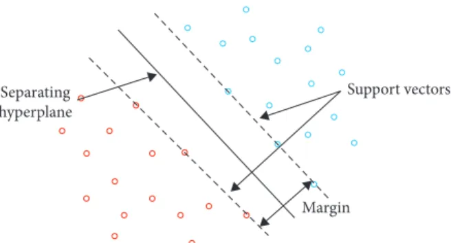
Support vector machines (SVMs) were introduced in [31], for classification problems. The objective is to look for the optimal separating hyperplane between classes. The points lying on classes’ boundaries are called support vectors, and the in-between space is called the hyperplane; when a linear separator is not able to find a solution, data points are projected into a higher-dimensional space, where the pre-vious nonlinearly separable points become linearly separa-ble, using kernel functions. The whole task can be formulated as a quadratic optimization problem that can be solved with exact techniques.
Figure 1 presents an example of a linearly separable classification problem solved using SVM. SVM aims at maximizing the margin between the support vectors and the hyperplane.
4.1. Support Vector Regression. One year after the
intro-duction of SVM, Smola et al. [32] advanced an alternative loss function, which also allowed SVM to be applied to regression problems. Support vector regression (SVR) has been applied in the field of TS forecasting, with excellent outcomes. For instance, Drucker et al. [22], M¨uller et al. [23], and Cao and Tay [33] suggest that SVR is a promising method for TS forecasting, as it offers several advantages: a smaller number of free parameters, better forecast ability, and faster training.
In SVR, the idea is to map the data events X into a k-dimensional feature space F, through a nonlinear mapping
φj(X), so that it is possible to fit a linear regression model to
the data points in this space. The obtained linear learner is then used to forecast in the new feature space. Once again, the mapping from the input space into the new feature space is defined by the kernel function.
One of the most attractive characteristics of SVR is related to the model errors; instead of minimizing the ob-served training error, SVR minimizes a combination of the training error and a regularization term, aimed at improving the generalization ability of the model [34]. Other attractive properties of SVR are related to the use of kernel functions, which make them applicable both to linear and nonlinear forecasting problems, and the absence of local minima in the error surface, due to the convexity of the fitness function and its constraints.
Given:
Training dataset T, represented by
T � x 1, y1, x2, y2, . . . , xm, ym, (1)
where x ∈ X ⊂ Rn are the training inputs and y∈ Y ⊂ R are the training expected outputs.
A nonlinear function:
f(x) � wTΦ xi + b, (2)
where w is the weight vector, b is the bias, and Φ(xi)is the
high dimensional feature space, which is linearly mapped from the input space x; the objective is to fit the training dataset T by finding a function f(x) that has the smallest possible deviation ε from the targets yi.
Equation (2) can be rewritten into a constrained convex optimization problem as follows:
minimize 1 2w T w subject to yi− wTΦ xi − b≤ ε wTΦ x i + b − yi≤ ε. ⎧ ⎪ ⎪ ⎨ ⎪ ⎪ ⎩ (3)
The aim of the objective function represented in equa-tion (3) is to minimize w while satisfying the other con-straints. One assumption is that f(x) exists, i.e., the convex optimization problem is feasible. This assumption is not always true; therefore, one might want to trade off errors by the flatness of the estimate. Having this in mind, Vapnik reformulated equation (3) as minimize 1 2w T w + C m i�1 ξ+i +ξ − i subject to yi− wTΦ x i − b≤ ε + ξ + i wTΦ x i + b − yi≤ ε + ξ − i ξ+iξ − i ≥ 0, ⎧ ⎪ ⎪ ⎪ ⎪ ⎪ ⎪ ⎪ ⎨ ⎪ ⎪ ⎪ ⎪ ⎪ ⎪ ⎪ ⎩ (4)
where C < 0 is a prespecified constant that is responsible for regularization and represents the weight of the loss function. The first term of the objective function wTw is the
regu-larized term, whereas the second term C mi�1(ξ +
i +ξ
−
i) is
called the empirical term and measures the ε-insensitive loss function.
To solve Equation (4), Lagrangian multipliers (∝+
i, ∝−i,η+i,η−i) can be used to eliminate some of the
primal variables. The final equation that translates the dual optimization problem of SVR is minimize 1 2 m i,j�1 K x i, xj ∝ + i −∝ − i ∝ + j − ∝ + j +ε m i�1 ∝+i +∝ − i − m i�1 ∝+i −∝ − i subject to m i�1 ∝+i −∝ − i �0 ∝+ i,∝ − i ϵ[0, C], ⎧ ⎪ ⎪ ⎪ ⎪ ⎨ ⎪ ⎪ ⎪ ⎪ ⎩ (5)
where K(xi, xj) is the kernel function; the above
formu-lation allows the extension of SVR to nonlinear functions, as the kernel function allows nonlinear function approxima-tions while maintaining the simplicity and computational efficiency of linear SVR.
The performance and good generalization of SVR de-pend on three training parameters:
The kernel function
C (the regularization parameter) ε (the insensitive zone)
Many possible kernels exist. In this work, the polynomial kernel and the radial basis function (RBF) kernel were studied. The interested reader is referred to [35] for a dis-cussion of these and other existing kernel functions.
5. Data Description
The dataset used in this study was extracted from EPA’s Air Quality [6]. All the files contain hourly data, separated by pollutant or parameter that is being measured—CO, SO2,
NO2, ozone, PM2.5, temperature, humidity, and wind, with Margin
Separating hyperplane
Support vectors
observations from the state of California. The hourly events were collected between January 1, 2016, and May 1, 2018. A total of 102090 records were used.
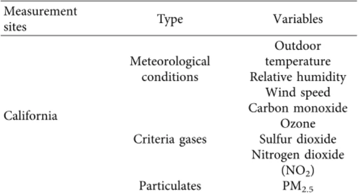
Tables 1 and 2 report a summary of the measured pa-rameters and sites and a detailed description of the variables used in the study:
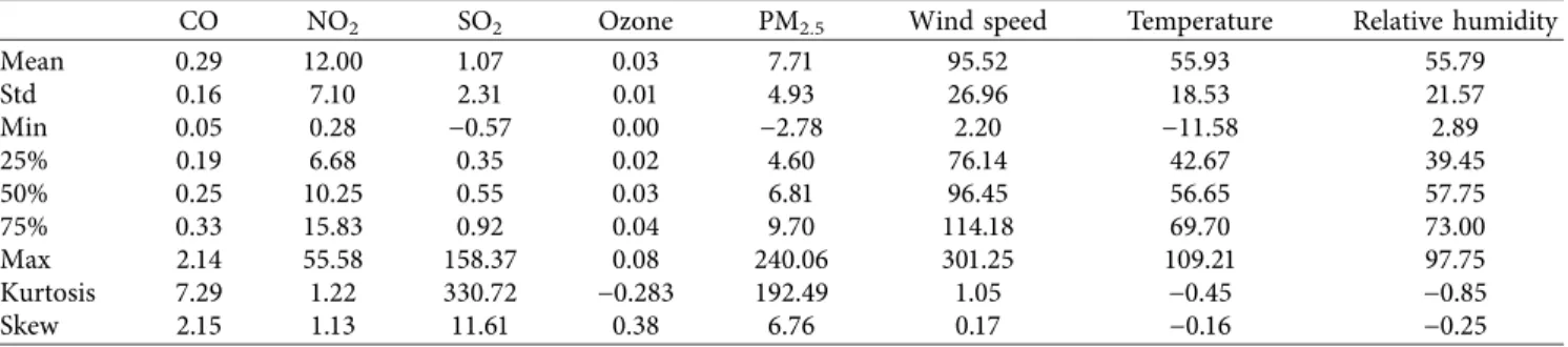
Table 3 provides a short descriptive statistic of the available pollutants, particles, and environment events measures: minimum, maximum, mean, standard deviation, quantiles, kurtosis, and skewness.
A high value of skewness for SO2indicates the presence
of sharp increases in the data. The high values in the kurtosis index for CO, SO2, and PM2.5confirm the existence of data
discontinuities. For SO2, the calculated standard deviation is
almost two times bigger than its mean, which means that, for this pollutant, the sensitivity to uncertainties is high.
Time plots are significantly important for an initial time-series analysis, as they serve as a descriptive tool that may show both trend and seasonality, potential outliers, or discontinuities, allowing us to make better decisions when it comes to choosing the appropriate technique to forecast the TS. Some visual representations of the data used in this work are shown in Figures 2 and 3.
From the plots, it can be observed that the distribution for each one of the pollutants and particulates is nonlinear. A series is stationary when the variance of it remains the same over time. The plots reported below seem to indicate the stationarity from the pollutants’ series. Furthermore, it is possible to identify the presence of outliers. One particular case is sulfur dioxide, in April 2017, with a measurement clearly above the regular series values. The time plots also portray the differences in terms of pollutant levels evolution across the years. For instance, SO2presents higher values for
the first semester of 2018.
6. Data Preprocessing
Data quality and its representativity are the first and most points to guarantee the successful building of fore-casting models. The data preprocessing step often impacts the generalization ability of a machine learning algorithm [36]. Data preprocessing usually encompasses missing data imputation, removing or modifying outlier observations, data transformation (often normalization and standardi-zation), and feature engineering. While the first two steps are useful to have more accurate and complete sets of data, the third one is typically used to have more uniformly dis-tributed data and to minimize data variability. Finally, the fourth step is used to obtain a new, typically smaller, and more informative dataset. This last step is typically com-posed of feature extraction and feature selection. In the continuation of this section, we describe how these steps were accomplished in this work.
6.1. Missing Data Imputation. In our dataset, the majority of
missing data is present in the qualifier variable for all pol-lutants, particles, and meteorological conditions, followed by CO sample measurements. Given the large number of
missing values for pollutants qualifier features, more than 50% of the total available events, it was decided to discard them from the dataset. For all the other categorical variables, it was decided to fill the missing values with the most common value from each feature, as suggested in [37]. We used the estimation of a 2ndorder polynomial to handle the
missing data for numerical variables (CO, SO2, NO2, PM2.5, outdoor temperature, relative humidity, and wind speed). This method was adopted because it outperformed the more traditional imputation using the series mean or linear in-terpolation (these preliminary experimental results are not shown here to save space).
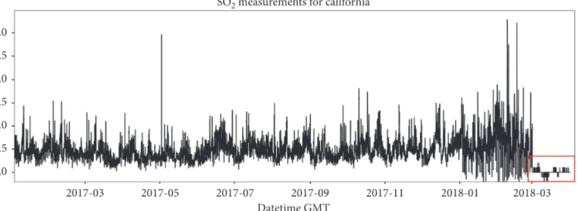
6.2. Removing Outliers. An irregular behavior was observed
in the SO2 series for the last months of 2018, as shown in
Figure 4, where the levels are much lower than expected. As these observations are outliers, the decision was to remove all the observations from March 2018 onwards, for the SO2series.
6.3. Data Transformation. We selected the Yeo-Johnson
power transformation method [38] to transform our data. This choice is motivated by the fact that, as reported in [39], the Yeo-Johnson method provides a nonlinear transfor-mation, less impacted by the presence of abnormal obser-vations. This option allowed us to obtain a dataset with improved features’ distribution and to minimize data variability.
6.4. Feature Extraction. The datetime component contained
in our dataset was used to obtain new features, valuable to help tease out series seasonality information. Considering all the properties that can be extracted from a datetime type of variable, the following new features were created: month number [1–12], hour of the day [0–23], and weekend added as a Boolean feature. As the hour of the day is, actually, a cyclical variable, it was decided to create two new features through a trigonometric approach, hour_sin � sin(2π hour/24) and hour_cos � cos(2π hour/24), to map this behavior. Finally, we created a variable called season, with four possible values for Fall, Winter, Spring, and Summer.
Table 1: Summary of measurement sites and observed variables. Measurement
sites Type Variables
California Meteorological conditions Outdoor temperature Relative humidity Wind speed Criteria gases Carbon monoxide Ozone Sulfur dioxide Nitrogen dioxide (NO2) Particulates PM2.5
The pollutant data are expressed in units of mass concentrations, i.e., mg/m3
Table 2: Dataset variable description.
Variable name Description
Stated name The state name where the monitor resides.
Parameter code The AQS code corresponding to the parameter being measured.
Parameter name The name or description assigned in AQS to the parameter measured by the monitor. The parameters are CO, SO2, NO2, ozone, PM2.5, temperature, humidity, and wind.
Date GMT The calendar date of the average in Greenwich Mean Time.
Time GMT The time of the day for the average on a 24-hour clock in Greenwich Mean Time.
Units of measure The units of measured parameter.
Uncertainty The reporting agency indicates the total measurement uncertainty associated with a reported measurement. Qualifier Sample values may have qualifiers that indicate why they are missing or that key is out of ordinary. Types of qualifiers
are null data, exceptional events, natural events, and quality assurance. Date of last
change The date the last time any numeric values in this record were updated in the AQS data system.
The pollutant data are expressed in units of mass concentrations, i.e., mg/m3(ppm), except for NO2, which is measured in ppb.
Table 3: Dataset descriptive statistics.
CO NO2 SO2 Ozone PM2.5 Wind speed Temperature Relative humidity
Mean 0.29 12.00 1.07 0.03 7.71 95.52 55.93 55.79 Std 0.16 7.10 2.31 0.01 4.93 26.96 18.53 21.57 Min 0.05 0.28 −0.57 0.00 −2.78 2.20 −11.58 2.89 25% 0.19 6.68 0.35 0.02 4.60 76.14 42.67 39.45 50% 0.25 10.25 0.55 0.03 6.81 96.45 56.65 57.75 75% 0.33 15.83 0.92 0.04 9.70 114.18 69.70 73.00 Max 2.14 55.58 158.37 0.08 240.06 301.25 109.21 97.75 Kurtosis 7.29 1.22 330.72 −0.283 192.49 1.05 −0.45 −0.85 Skew 2.15 1.13 11.61 0.38 6.76 0.17 −0.16 −0.25
SO2 measurements for the state of california 3.0 2.5 2.0 1.5 1.0 0.5 0.0 –0.5 2016-03 2016-06 2016-09 2016-12 2017-03 2017-06 2017-09 2017-12 2018-03 Datetime GMT
Figure 2: Sulfur dioxide measurements for the state of California.
Carbon monoxide measurements for the state of california 1.50 1.25 1.00 0.75 0.50 0.25 0.00 –0.25 2016-03 2016-06 2016-09 2016-12 2017-03 2017-06 2017-09 2017-12 2018-03 Datetime GMT
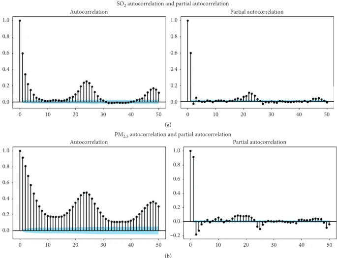
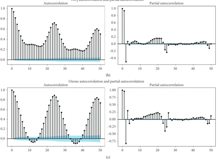
In time-series analysis, lags are considered a backshift in the series and are useful to measure an important phe-nomenon, called series autocorrelation. The selection of appropriate time lags for forecasting is an important step, through the elimination of redundant features. This pro-cedure generally helps improve the overall forecasting model accuracy and gives a better understanding of the underlying process [40]. An exploratory study was conducted using autocorrelation function (ACF) and partial autocorrelation function (PACF), commonly used in time-series analysis, to define the number of lag variables per pollutant and particle. As one can notice in Figures 5 and 6, the ACF plots show a repeating pattern every 24 hours, while the PACF plots present spikes in the first two lags and a decrease for all the others lags. Assuming a confidence level of 80%, only the first and the second lag were considered as relevant for all the pollutants series, resulting in a total of 10 new variables. Finally, the last featured variables regard each pollutant series rolling mean, with a 24 lag time window.
The total extracted features encompass variables related to pollutant and particulate measurements, meteorological conditions, lag features, rolling mean variables, season time, and time-related variables. Finally, the complete dataset contains 46 features, including the ones added in the feature extraction phase. In particular, in the feature extraction phase, the following variables were created: ten lag variables for the pollutant series, five rolling mean variables (one for each pollutant), one variable for the season, four trigono-metric variables (two for the month and two for the hour), one Boolean variable for the weekend, and variables for the date and time.
6.5. Feature Selection. From the 46 features resulting from
the feature engineering process described above, variable selection was performed to reduce dataset dimensionality and eliminate the presence of collinearity. As reported in [41], air pollutant concentration, including ground-level ozone, PM2.5, and NO2, varies depending on meteorological
factors and the local topography. Meteorological conditions, in particular, can impact the concentrations, as they have complex interactions between the various processes such as air pollutant emission, transportation, chemical
transformations, disposition (wet and dry), and dispersion [42]. For this reason, all variables relative to meteorological conditions were kept in the dataset. On the other hand, both filters and embedded methods were used to select all the other features. Filters are methods that perform feature selection regardless of the forecasting model chosen; em-bedded methods perform variable selection based on the chosen learning method (SVR in our case).
With respect to filters, the Pearson correlation-based feature selection was used, as suggested in [43]. This method was employed to verify the existence of collinearity between the available features. We discovered that some pollutants in the dataset present an almost linear relationship between their observations; this is the case for NO2and CO and even
between CO and PM2.5. Based on the strong correlation
between pollutants and their natural dependence, as referred by Cagliero et al. [44], it was decided to keep all pollutants in the dataset. Since pollutants’ respective lag variables hold high variance between them, it was decided only to use the target pollutants’ respective lag features to avoid possible collinearity between features.
Furthermore, although SVR is known to be robust in terms of collinearity and multicollinearity [45], some re-dundant variables were excluded to reduce dataset di-mensionality. In particular, the variable referring to the month number presents a high correlation with some pollutants, the same for month cyclical variables (Month_cos and Month_sin). Thus, we eliminated the variable month. An analogous decision was taken for data concerning hour information, with variables Hour_sin and Hour_cos chosen and variable hour eliminated. The sea-son-related features were also excluded from the dataset, given their linear correlation with Month_cos and Month_sin and features reporting on the meteorological conditions. Also, both quarter and weekday were removed, due to a high correlation with the month cyclic and Is_Weekend features.
The objective of our work is to generate different forecasting models for five different pollutants: CO, NO2,
SO2, ozone, and PM2.5. Table 4 summarizes the features that
were maintained in the dataset for the forecasting of each one of these pollutants (features that were maintained in the dataset are marked with “∗” in the table).
SO2 measurements for california 3.0 2.5 2.0 1.5 1.0 0.5 0.0 2017-03 2017-05 2017-07 2017-09 2017-11 2018-01 2018-03 Datetime GMT
1.0 0.8 0.6 0.4 0.2 0.0 1.0 0.8 0.6 0.4 0.2 0.0 0 10 20 30 40 50 0 10 20 30 40 50
Autocorrelation Partial autocorrelation
SO2 autocorrelation and partial autocorrelation
(a) 1.0 0.8 0.6 0.4 0.2 0.0 1.0 0.8 0.6 0.4 0.2 –0.2 0.0 0 10 20 30 40 50 0 10 20 30 40 50
Autocorrelation PM2.5 autocorrelation and partial autocorrelationPartial autocorrelation
(b)
Figure 5: ACF and PACF plots for SO2and PM2.5in California.
Autocorrelation Partial autocorrelation
1.0 0.8 0.6 0.4 0.2 0.0 –0.2 –0.4 –0.6
CO autocorrelation and partial autocorrelation
0 10 20 30 40 50 0 10 20 30 40 50 1.0 0.8 0.6 0.4 0.2 0.0 (a) Figure 6: Continued.
1.0 0.8 0.6 0.4 0.2 0.0 –0.2 –0.4
Autocorrelation NO2 autocorrelation and partial autocorrelation Partial autocorrelation
0 10 20 30 40 50 0 10 20 30 40 50 1.0 0.8 0.6 0.4 0.2 0.0 (b) 1.00 0.75 0.50 0.25 0.00 –0.25 –0.50 –0.75
AutocorrelationOzone autocorrelation and partial autocorrelation Partial autocorrelation
0 10 20 30 40 50 0 10 20 30 40 50 1.0 0.8 0.6 0.4 0.2 0.0 (c)
Figure 6: ACF and PACF plots for CO, NO2, and ozone in California.
Table 4: Selected variables’ summary per target variable.
Features Pollutants and particulates
CO NO2 SO2 Ozone PM2.5 CO ∗ NO2 ∗ SO2 ∗ Ozone ∗ PM2.5 ∗ Wind speed ∗ ∗ ∗ ∗ ∗ Relative humidity ∗ ∗ ∗ ∗ ∗ Outdoor temperature ∗ ∗ ∗ ∗ ∗ CO roll mean ∗ CO lag features ∗ ∗ ∗ ∗ ∗ SO2_roll_mean ∗ SO2lag features ∗ ∗ ∗ ∗ ∗ NO2_roll_mean ∗ NO2lag features ∗ ∗ ∗ ∗ ∗
Ozone lag features ∗ ∗ ∗ ∗ ∗
Ozone roll mean ∗
PM2.5lag features ∗ ∗ ∗ ∗ ∗ PM2.5roll mean ∗ Is_Weekend ∗ ∗ ∗ ∗ ∗ Hour_sin ∗ ∗ ∗ ∗ ∗ Hour_cos ∗ ∗ ∗ ∗ ∗ Month_sin ∗ ∗ ∗ ∗ ∗ Month_cos ∗ ∗ ∗ ∗ ∗
Table 5: Random search optimal parameter results per pollutant dataset.
Pollutants PCA dataset Normalized dataset
Kernel Opt C Opt ε R2 Kernel Opt C Opt ε R2
CO RBF 3 0.08 0.783 RBF 2 0.033 0.916
NO2 RBF 3 0.025 0.882 RBF 1 0.067 0.948
SO2 RBF 1 0.062 0.712 RBF 2 0.086 0.718
Ozone RBF 2 0.076 0.903 RBF 2 0.02 0.979
PM2.5 RBF 1 0.055 0.765 RBF 3 0.032 0.767
Carbon monoxode boxplot prediction comparision
Normalized data Denormalized data
CO_pt Predicted_CO_PCA (a) (b) Predicted_CO CO_pt_denorm Predicted_CO_PCA_denorm Predicted_CO_denorm 4 3 2 1 0 –1 –2 1.0 0.8 0.6 0.4 0.2
Figure 7: Boxplot of predicted and observed carbon monoxide values.
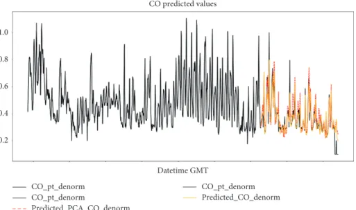
Datetime GMT 1.0 0.8 0.6 0.4 0.2 CO predicted values CO_pt_denorm Predicted_CO_denorm CO_pt_denorm CO_pt_denorm Predicted_PCA_CO_denorm Datetime GMT
Figure 8: Forecasts of carbon monoxide measurements in California using the produced SVR forecasting models. The black line shows the observed values, whereas the red and yellow lines show the produced forecasts.
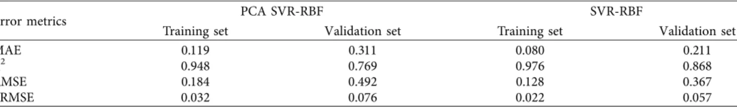
Table 6: Error metrics from CO forecasting models in the training and validation sets.
Error metrics PCA SVR-RBF SVR-RBF
Training set Validation set Training set Validation set
MAE 0.119 0.311 0.080 0.211 R2 0.948 0.769 0.976 0.868 RMSE 0.184 0.492 0.128 0.367 nRMSE 0.032 0.076 0.022 0.057 2018-01-02 2018-01-04 2018-01-06 2018-01-08 2018-01-10 2018-01-12 2018-01-14 1.0 0.8 0.6 0.4 0.2
CO detailed period predictions
Datetime GMT CO_pt_denorm
Predicted_PCA_CO_denorm Predicted_CO_denorm
(a) Carbon monoxide PCA error plot
0.2 0.4 0.6 0.8 1.0 0.2 0.0 –0.2 –0.4 –0.6 Resid uals (p re dic te d-obs er ve d)
Carbon monoxide observed values (b)
Carbon monoxide error plot
0.2 0.4 0.6 0.8 1.0 0.2 0.0 –0.2 –0.4 –0.6 Resid uals (p re dic te d-obs er ve d)
Carbon monoxide observed values (c)
Figure 9: (a) Carbon monoxide forecast detail between the period of the 1st of January and the 15th. Both forecasting methods missed to forecast some of the spikes registered in the series in the beginning of January. (b, c) Two scatter plots with model’s respective errors plotted against observed CO values for the same period.
Given a total of 40 dependent variables for each target pollutant and as per the existence of collinearity between variables, it was also decided to apply principal component analysis (PCA) [46] to reduce the dataset dimensionality. The datasets for each pollutant prediction were reduced in approximately 77.5% of their size through the application of PCA. In the experimental study presented in the next sec-tion, SVR will be applied both to the dataset containing all the 40 dependent variables and to the dataset that was re-duced through PCA.
7. Experimental Study
7.1. Experimental Settings. As discussed above, SVM has
three hyperparameters that need to be user-defined: the kernel type function, the regularization constant C, and the maximum allowed deviation ε. Time-series split combined with random grid search was used to obtain the optimal numbers for both C and ε, similar to what was done in [47, 48]. According to [33], the appropriate range for the C parameter should be between 10 and 100; in order to have a wider exploration of this parameter, the search range for C was extended to [1, 100]. The range defined for ε was between 0.001 and 0.1, with a step of 0.001. The most frequently used kernel functions, as discussed previously, are polynomial and RBF. For that reason, both were used in random grid search.
The number of iterations chosen to run the random search was selected based on [49], reporting that random search needs 60 iterations, on average, to achieve results as good as the ones achieved by the grid-search algorithm. Table 5 shows the results of the random search.
As shown in Table 5, different values of C and ε were obtained for the different pollutants; on the other hand, the RBF kernel consistently returned the best results. For this reason, from now on, only the RBF kernel will be considered. So, in the next section, two types of results will be analyzed and compared between each other: those obtained by SVR with RBF kernel on the dataset without application of the PCA (SVR-RBF from now on) and those obtained by SVR with RBF kernel on the dataset filtered by PCA (PCA SVR-RBF from now on). We utilized the Pearson correlation, the mean ab-solute error (MAE), the root mean squared error (RMSE), and the normalized RMSE (nRMSE) as measures to compare these two models between each other. The models were trained using 70% of the available data, which correspond to the period between 02-01-2018 at 08 : 00 : 00 and 07-08-2017 at 00 : 00 : 00. The validation set is composed of the remaining 30% of the observations, which is relative to the period between 07-08-2017 at 01 : 00 : 00 and 01-03-2018 at 23 : 00 : 00.
7.2. Experimental Results. In this section, we report and
discuss the experimental results achieved by SVR-RBF and PCA SVR-RBF in the forecasting of five different
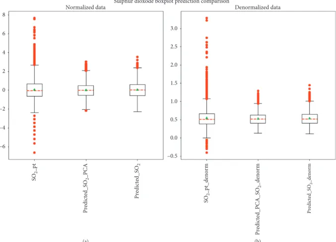
8 6 4 2 0 –2 –4 –6 3.0 2.5 2.0 1.5 1.0 0.5 0.0 –0.5 (a) (b) SO 2 _pt Predicted_SO 2 _PCA Predicted_SO 2 SO 2 _pt_denorm Predicted_PCA_SO 2 _denorm Predicted_SO 2 _denorm
Sulphur dioxode boxplot prediction comparison
Normalized data Denormalized data
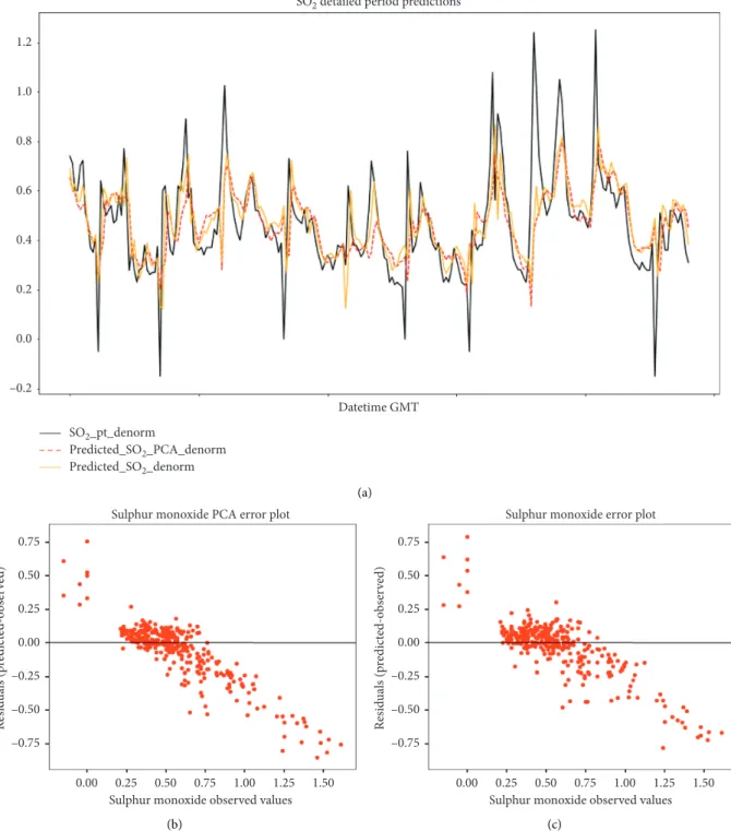
Datetime GMT SO2_pt_denorm Predicted_SO2_PCA_denorm Predicted_SO2_denorm 1.2 1.0 0.8 0.6 0.4 0.2 0.0 –0.2
SO2 detailed period predictions
(a) 0.75 0.50 0.25 0.00 –0.25 –0.50 –0.75 Resid uals (p re dic te d-obs er ve d)
Sulphur monoxide PCA error plot
Sulphur monoxide observed values 0.00 0.25 0.50 0.75 1.00 1.25 1.50 (b) 0.75 0.50 0.25 0.00 –0.25 –0.50 –0.75 Resid uals (p re dic te d-obs er ve d)
Sulphur monoxide error plot
Sulphur monoxide observed values 0.00 0.25 0.50 0.75 1.00 1.25 1.50
(c)
Figure 11: (a) Sulfur dioxide forecasts in California using the produced SVR forecasting models as well as the observed SO2values. The black line shows the observed values and the red line shows the produced forecasts with the PCA model, whereas the yellow line shows the forecast produced with the normalized dataset. (b, c) Two scatter plots with model’s respective errors plotted against observed SO2values for the same period.
Table 7: Error metrics from SO2forecasting models in the training and validation sets.
Error metrics PCA SVR-RBF SVR-RBF
Training set Validation set Training set Validation set
MAE 0.236 0.461 0.229 0.414
R2 0.787 0.023 0.830 0.273
RMSE 0.364 0.752 0.352 0.703
pollutants (CO, NO2, SO2, ozone, and PM2.5, Sections
7.2.1 to 7.2.5, respectively) and the forecasting of the air quality index (AQI) (Section 7.2.6). The software used for performing this experimental phase was developed in Python (version 3.6), mainly using the Pandas and Scikit-learn packages.
7.2.1. Carbon Monoxide (CO). The results obtained for the
forecasting of carbon monoxide are shown in the boxplots of Figure 7. Median, first, and third quantiles and maxi-mum and minimaxi-mum values of the prediction, together with the value of the expected output, are reported. The leftmost plot shows the results obtained before applying the inverse Yeo-Johnson power transformation (indicated as “nor-malized data” in the figure), whereas the right side reports
the data after this transformation (indicated as “denor-malized data” in the figure). Inside both these plots, three boxplots are shown: the leftmost one reports the observed CO values, the one in the middle shows the predicted values returned by PCA SVR-RBF, and the rightmost boxplot reports the predicted values returned by SVR-RBF. The obtained predictions have very close median values to the observed carbon monoxide both for PCA SVR-RBF and SVR-RBF. However, the observed CO values present a higher quantity of extreme observations that the fore-casting models tend to underestimate. Figure 8 shows the forecasted values produced by both PCA SVR-RBF (red line) and SVR-RBF (yellow line). The carbon monoxide forecast error statistics are shown in Table 6. The values predicted by the SV-RBF model are slightly lower than the ones obtained by the PCA SVR-RBF model, although both
3 2 1 0 –1 –2 –3 NO 2 _pt Predicted_NO 2 _PCA Predicted_NO 2 NO 2 _pt_denorm Predicted_NO 2 _PCA_denorm Predicted_NO 2 _denorm 35 30 25 20 15 10 (a) (b) 5 0
Nitrogen dioxode boxplot prediction comparison
Normalized data Denormalized data
Figure 12: Boxplot representation of observed and forecasted nitrogen dioxide values (PCA SVR-RBF and SVR-RBF values, before and after Yeo-Johnson power transformation).
Table 8: Error metrics from NO2forecasting models in the training and validation sets.
Error metrics PCA SVR-RBF SVR-RBF
Training set Validation set Training set Validation set
MAE 0.106 0.229 0.095 0.162
R2 0.975 0.885 0.981 0.937
RMSE 0.150 0.316 0.132 0.238
forecasting models achieved good results on the validation dataset. In Figure 9, both the observed values and obtained predictions for the period between January 1st and January 15th are reported, as well as the obtained errors, which allow us to understand that the highest error values occurred when the highest spikes of carbon monoxide values were registered. Overall, both studied forecasting models achieved good per-formance in predicting the carbon monoxide values observed in California.
7.2.2. Sulfur Dioxide (SO2). The results obtained for sulfur
dioxide by PCA SVR-RBF and SVR-RBF are shown in Figure 10. This figure reveals that both PCA SVR-RBF and
SVR-RBF can predict the observed SO2 values with good
accuracy. PCA SVR-RBF forecasts present a relatively smaller gap between quartiles when compared with SVR-RBF. Also, considering extreme values, the observed values have a higher incidence of outliers when compared with the forecasts, which indicates that both PCA SVR-RBF and SVR-RBF tend to underpredict the observed values slightly. Figure 11 shows forecasts for PCA SVR-RBF (red line) and SVR-RBF (yellow line). The sulfur dioxide forecast error statistics are shown in Table 7.
Similar to carbon monoxide, the residual metrics present lower values for the SVR-RBF model. From Figure 11, it is possible to observe that both models missed predicting the frequent high spikes present in the observed values. This
30 25 20 15 10 5 0 NO2 predicted values Datetime GMT NO2_pt_denorm Predicted_NO2_denorm NO2_pt_denorm NO2_pt_denorm Predicted_PCA_NO2_denorm (a) 5.0 2.5 0.0 –2.5 –5.0 –7.5 –10.0 –12.5
Nitrogen dioxide observed values
5 10 15 20 25 Resid uals (p re dic te d-obs er ve d)
Nitrogen dioxide PCA error plot
(b)
Nitrogen dioxide observed values
5 10 15 20 25 5.0 2.5 0.0 –2.5 –5.0 –7.5 –10.0 –12.5 Resid uals (p re dic te d-obs er ve d)
Nitrogen dioxide error plot
(c)
Figure 13: (a) Nitrogen dioxide observed values (black line) and obtained forecasts with PCA-SVR model (red line) and SVR-RBF model (yellow line). (b, c) Two scatter plots with model’s respective errors plotted against observed NO2values for the same period.
result is also corroborated by the error scatter plots from both forecasting models. The error scatter plots (Figures 11(b) and 11(c)) allow us to understand that most of the errors are between the range of [0.25; −0.25] ppb, al-though there are very high error values which occur mainly for the higher and lower observed values. It is also possible to corroborate that both models tend to underpredict the registered pollutant values, given that we observe the highest concentration of points below zero.
7.2.3. Nitrogen Dioxide (NO2). Figure 12 depicts the boxplot
representations for the observed values and the predicted values with both PCA SVR-RBF and SVR-RBF. The presented
boxplots have approximately the same median values as well as the same data variability. As regards extreme observations, the raw NO2 dataset has more identified outliers above the 3rd
quantile, when compared with the forecasted values. The re-sults concerning MAE, nRMSE, and R2are shown in Table 8. In Figure 13, the observed NO2 values, as well as the obtained
predictions, are reported (top figure plot). Figures 13(b) and 13(c) show the forecasting models’ errors, respectively, plotted against the nitrogen dioxide observed values. As expected, both forecasting models can capture the pollutant behavior very well, although PCA SVR-RBF tends to underpredict the ob-served values spikes. In conclusion, both models trained to forecast nitrogen dioxide achieved good results, with SVR-RBF slightly outperforming PCA SVR-RBF.
Table 9: Forecasting models’ error metrics for ozone measurement in the training and validation sets.
Error metrics PCA SVR-RBF SVR-RBF
Training set Validation set Training set Validation set
MAE 0.083 0.190 0.041 0.088 R2 0.987 0.923 0.996 0.982 RMSE 0.110 0.262 0.060 0.133 nRMSE 0.023 0.050 0.013 0.025 3 2 1 0 –1 –2 0.07 0.06 0.05 0.04 0.03 0.02 0.01 Ozone_pt Predicted_PCA_ozone Predicted_ozone Ozone_pt_denorm Predicted_PCA_ozone_denorm Predicted_ozone_denorm
Ozone boxplot prediction comparision Normalized data
(a) (b)
Denormalized data
Figure 14: Boxplot representation of observed and forecasted ground-level ozone values (PCA and normalized dataset, before and after Yeo-Johnson power transformation).
7.2.4. Ground-Level Ozone. The observed ground-level
ozone values and corresponding predictions are shown in Figure 14. The represented boxplots have approximately the same median values and box size. A small number of outliers were identified in ozone’s observed values, different from the forecasts that have, almost, no outlier observation. Forecast performance metrics are shown in Table 9. In Figure 15, we report the observed ozone values and the obtained predicted values from both PCA SVR-RBF and SVR-RBF during the period between January 1st and January 15th. For this pe-riod, it is possible to observe that the PCA SVR-RBF tends to forecast higher ozone values compared to the observed ones, while the SVR-RBF seems to model the ozone measurements more accurately. Figure 16 reports the forecasting model’s
errors, plotted against the observed ozone values. As ex-pected, based on the results shown in Table 9, ozone measurements were modeled with very good results by both forecasting models, with SVR-RBF scatter plot points more concentrated around null values. In conclusion, both models trained to predict ozone measurements achieved very good results, but SVR-RBF slightly outperformed PCA SVR-RBF.
7.2.5. Particulate Matter 2.5 (PM2.5). The last pollutant
forecast evaluation that we performed concerns particulate matter 2.5. Similar to the evaluation of the other pollutants, in Figure 17, we report the boxplots for both observations and predictions. The boxplots of the medians are
2018-01-02 2018-01-04 2018-01-06 2018-01-08 2018-01-10 2018-01-12 2018-01-14 Datetime GMT
Ozone detailed period predictions
Ozone_pt_denorm Predicted_PCA_ozone_denorm Predicted_ozone_denorm 0.035 0.030 0.025 0.020 0.015 0.010
Figure 15: Observed and predicted ozone values for the period between January 1st and January 15th.
0.015 0.010 0.005 0.000 –0.005 –0.010 Residuals (predicted-observed) 0.005 0.010 0.015 0.020 0.025 0.030 0.035 0.040 Ozone observed values
Ozone PCA error plot
(a) 0.015 0.010 0.005 0.000 –0.005 –0.010 Residuals (predicted-observed) 0.005 0.010 0.015 0.020 0.025 0.030 0.035 0.040 Ozone observed values
Ozone error plot
(b)
Figure 16: (a) PCS SVR-RBF forecasting errors plotted against observed ozone values and (b) SVR-RBF forecasting errors plotted against observed ozone values.
approximately the same for observed and forecast values, but the amount of outlier observations in the raw PM2.5data is
higher, which indicates that both forecasting models are underpredicting observed spikes for this pollutant. Fore-casting errors are shown in Table 10. Both models present slightly bigger values in MAE in the validation set when compared to the results obtained on the training set. In Figure 18, we report the observed values and the forecasts produced by PCA SVR-RBF and SVR-RBF for the period between January 1st and January 15th. From this figure, it is possible to see that both models underpredicted the high values of PM2.5. Figure 19 shows the forecasting model’s
errors plotted against observed PM2.5values. As expected,
the observed PM2.5 values were not correctly modeled
whenever the series of observed events presented an ab-normally high value, as both scatter plots present a positive correlation between the high residual values and high PM2.5
observations. To summarize, both studied models achieved similar performance when predicting particulate matter 2.5, with SVR-RBF outperforming PCA SVR-RBF.
7.2.6. Air Quality Index (AQI). The AQI, as previously
pointed out, is an index used by government agencies to quantify the level of pollution of air. According to the EPA (the United States Environmental Protection Agency), AQI values range from 0 to 500, where the greater the AQI, the greater the pollution. AQI values should be understood according to the classification reported in Table 11.
Based on the observed values of the pollutants and the predicted values, the AQI value per hour was calculated for the training and validation sets. In Tables 12 and 13, we report the confusion matrix that both models (PCA
SVR-Table 10: Forecasting models’ error metrics for particulate matter 2.5 measurements in the training and validation sets.
Error metrics PCA SVR-RBF SVR-RBF
Training set Validation set Training set Validation set
MAE 0.200 0.382 0.144 0.331 R2 0.882 0.563 0.937 0.647 RMSE 0.273 0.576 0.205 0.512 nRMSE 0.041 0.074 0.031 0.066 4 3 2 1 0 –1 –2 –3 50 40 30 20 10 0 PM2_5pt Predicted_PM2_5_PCA Predicted_PM2_5 (a) (b) PM2_5_pt_denorm Predicted_PM2_5_PCA_denorm Predicted_PM2_5_denorm
Particulate matter 2.5 boxplot predictions comparision
Normalized data Denormalized data
Figure 17: Boxplots of observed and forecasted particulate matter 2.5 values (PCA SVR-RBF and SVR-RBF, before and after Yeo-Johnson power transformation).
RBF and SVR-RBF) obtained in the training and the vali-dation datasets, respectively.
The PCA SVR-RBF model achieved an accuracy of 88% on the training set and 92.7% on the validation set, whereas SVR-RBF achieved a slightly better accuracy score for both datasets, with 90.02% on the training set and 94.1% on the validation set.
Considering the obtained results for both models (PCA SVR-RBF and SVR-RBF) for the cases that the AQI
was misidentified, Table 14 shows if the pollutant with the max AQI was correctly identified. For all cases where both the AQI classification and pollutant with the maximum AQI were misidentified, the pollutant with the second highest registered hourly AQI was always the correct one.
Interestingly, we observe that for both PCA SVR-RBF and SVR-RBF, all the AQI misclassifications happened when the observed particulate matter 2.5 values registered the
0 5 10 15 20 25 30 35 40 PM2.5 observed values 10 5 0 –5 –10 –15 –20 Residuals (predicted-observed)
PM2.5 PCA error plot
(a) 0 5 10 15 20 25 30 35 40 PM2.5 observed values 10 5 0 –5 –10 –15 –20 Residuals (predicted-observed) PM2.5 error plot (b)
Figure 19: (a) PCA SVR-RBF forecasting errors plotted against observed PM2.5values and (b) SVR-RBF forecasting errors plotted against observed PM2.5values.
PM2.5 detailed period predictions
2018-01-02 2018-01-04 2018-01-06 2018-01-08 2018-01-10 2018-01-12 2018-01-14 Datetime GMT PM2_5_pt_denorm Predicted_PCA_PM2_5_denorm Predicted_PM2_5_denorm 40 35 30 25 20 15 10 5 0
Table 14: AQI misidentified cases breakdown.
PCA SVR-RBF SVR-RBF
Training set Validation set Training set Validation set
Pollutant correctly identified? True 449 123 370 99
False 29 1 19 1
Table 11: The six AQI categories defined by EPA. Air quality index
value range Levels of health concern Description
0 to 50 Good Air quality is considered satisfactory.
51 to 100 Moderate
Air quality is acceptable; however, for some pollutants, there is a moderate health concern for a small number of people, namely, those that experience
respiratory problems.
101 to 150 Unhealthy for sensitive groups
Although for most of the people, the health concern is moderate, for groups with lung diseases, the elderly, and children, there is a great risk of exposure to
some pollutants and particulates.
151 to 200 Unhealthy Health side effects for all the affected area population. Sensitive groups may
experience more serious effects.
201 to 300 Very unhealthy Health alerts would be triggered as all the affected area population would experience serious health effects.
301 to 500 Hazardous Health alerts with emergency warnings would be triggered. The entire area
population would be severely affected.
Table 12: Confusion matrix for the AQI classifications obtained with both models for the training set.
Training dataset PCA SVR-RBF SVR-RBF
Good Moderate Unhealthy∗ Good Moderate Unhealthy∗
Good 2507 151 0 2549 109 0
Moderate 300 993 0 253 1040 0
Unhealthy∗ 4 23 0 9 18 0
∗Unhealthy for sensitive groups.
Table 13: Confusion matrix for the AQI classifications obtained with both models for the validation set.
Validation dataset PCA SVR-RBF SVR-RBF
Good Moderate Unhealthy∗ Good Moderate Unhealthy∗
Good 1161 59 0 1171 49 0
Moderate 62 420 0 48 434 0
Unhealthy∗ 0 3 0 0 3 0
maximum hourly AQI. In other words, the predictive models were not able to predict abnormal PM2.5 values.
To summarize, both PCA SVR-RBF and SVR-RBF achieved similar performance in forecasting the AQI. Nevertheless, there is an underestimation of the pollution levels when the highest AQI values were registered by PM2.5,
which would imply that pollution alerts would not be sent to the affected population groups in those cases.
8. Conclusions and Future Work
Predicting the air quality is a complex task due to the dy-namic nature, volatility, and high variability in space and time of pollutants and particulates. At the same time, being able to model, predict, and monitor air quality is becoming more and more important, especially in urban areas, due to the observed critical impacts of air pollution for populations and the environment.
This work presented a study of support vector regression (SVR) to forecast pollutants and particulates’ levels and to correctly identify the AQI. The studied method produced a suitable model of the hourly atmospheric pollution, allowing us to obtain, generally, good accuracy in modeling pollutant concentrations like O3, CO, and SO2, as well as the hourly
AQI for the state of California.
As future work, we intend to improve and investigate the usage of SVR to forecast air quality through the following topics:
Dataset and variable selection—considering a large dataset with more parameters and measurements, which can support more accurate predictive models for air pollutants and particulates, in particular, NO2and
PM2.5.
SVR parameter optimization—as SVR model perfor-mance is greatly influenced by the kernel function selection and the penalty parameter C, it would be interesting to explore other methods, different from random search, for hyperparameter optimization such as genetic algorithms or particle swarm optimization. Last but not least, we intend to compare the results obtained by SVR to the ones achieved by other machine learning algorithms of a different nature, like artificial neural networks, Bayesian networks, decision trees, random forests, and genetic programming.
Data Availability
A permanent link to download data used in this paper will be made available after the publication.
Conflicts of Interest
The authors declare that they have no conflicts of interest.
Acknowledgments
This study was supported by national funds by FCT (Fundação para a Ciˆencia e a Tecnologia) through projects
GADgET (DSAIPA/DS/0022/2018), BINDER (PTDC/CCI-INF/29168/2017), and AICE (DSAIPA/DS/0113/2019) and the LASIGE Research Unit (UIDB/00408/2020 and UIDP/ 00408/2020). Mauro Castelli and Aleˇs Popoviˇc acknowledge the financial support from the Slovenian Research Agency (research core funding no. P5-0410).
References
[1] U. A. Hvidtfeldt, M. Ketzel, M. Sørensen et al., “Evaluation of the Danish AirGIS air pollution modeling system against measured concentrations of PM2.5, PM10, and black carbon,” Environmental Epidemiology, vol. 2, no. 2, 2018.
[2] Y. Gonzalez, C. Carranza, M. Iniguez et al., “Inhaled air pollution particulate matter in alveolar macrophages alters local inflammatory cytokine and peripheral IFN pro-duction in response to mycobacterium tuberculosis,” Amer-ican Journal of Respiratory and Critical Care Medicine, vol. 195, p. S29, 2017.
[3] L. Pimpin, L. Retat, D. Fecht et al., “Estimating the costs of air pollution to the National Health Service and social care: an assessment and forecast up to 2035,” PLoS Medicine, vol. 15, no. 7, Article ID e1002602, pp. 1–16, 2018.
[4] F. Caiazzo, A. Ashok, I. A. Waitz, S. H. L. Yim, and S. R. H. Barrett, “Air pollution and early deaths in the United States. Part I: quantifying the impact of major sectors in 2005,” Atmospheric Environment, vol. 79, pp. 198–208, 2013. [5] B. Holmes-gen and W. Barrett, Clean Air Future, Health and
Climate Benefits of Zero Emission Vehicles, American Lung Association, Chicago, IL, USA, 2016.
[6] US Environmental Protection Agency (US EPA), “Criteria air pollutants,” America’s Children and the Environment, US EPA, Washington, DC, USA, 2015.
[7] CERN, Air Quality Forecasting, CERN, Geneva, Switzerland, 2001.
[8] G. E. Box and D. A. Pierce, “Distribution of residual auto-correlations in autoregressive-integrated moving average time series models,” Journal of the American statistical Association, vol. 65, no. 332, pp. 1509–1526, 1970.
[9] C. L. Hor, S. J. Watson, and S. Majithia, “Daily load fore-casting and maximum demand estimation using ARIMA and GARCH,” in Proceedings of the 2006 International Conference on Probabilistic Methods Applied to Power Systems, pp. 1–6, IEEE, Stockholm, Sweden, June 2006.
[10] L. Y. Siew, L. Y. Chin, P. Mah, and J. Wee, “Arima and in-tegrated arfima models for forecasting air pollution index in shah alam , selangor,” The Malaysian Journal of Analytical Science, vol. 12, no. 1, pp. 257–263, 2008.
[11] J. Zhu, “Comparison of ARIMA model and exponential smoothing model on 2014 air quality index in yanqing county, Beijing, China,” Applied and Computational Mathematics, vol. 4, no. 6, p. 456, 2015.
[12] T. M. Mitchell, “Machine learning,” in Proceedings of the IJCAI International Joint Conference on Artificial Intelligence, Pasadena, CA, USA, July 2009.
[13] U. Brunelli, V. Piazza, L. Pignato, F. Sorbello, and S. Vitabile, “Three hours ahead prevision of SO2 pollutant concentration using an Elman neural based forecaster,” Building and En-vironment, vol. 43, no. 3, pp. 304–314, 2008.
[14] G. Bontempi, S. Taieb, Y. Le Borgne, and D. Loshin, “Machine learning strategies for time series forecasting,” in Business Intelligence, pp. 59–73, Springer, Berlin, Germany, 2013. [15] R. Sharda and R. B. Patil, “Neural networks as forecasting
Joint Conference on Neural Networks, pp. 491–494, San Diego, CA, USA, January 1990.
[16] I. Alon, M. Qi, and R. J. Sadowski, “Forecasting aggregate retail sales:,” Journal of Retailing and Consumer Services, vol. 8, no. 3, pp. 147–156, 2001.
[17] L. A. D´ıaz-Robles, J. C. Ortega, J. S. Fu et al., “A hybrid ARIMA and artificial neural networks model to forecast particulate matter in urban areas: the case of Temuco, Chile,” Atmospheric Environment, vol. 42, no. 35, pp. 8331–8340, 2008.
[18] M. Cai, Y. Yin, and M. Xie, “Prediction of hourly air pollutant concentrations near urban arterials using artificial neural network approach,” Transportation Research Part D: Trans-port and Environment, vol. 14, no. 1, pp. 32–41, 2009. [19] J. C. M. Pires, M. C. M. Alvim–Ferraz, M. C. Pereira, and
F. G. Martins, “Prediction of PM10 concentrations through multi-gene genetic programming,” Atmospheric Pollution Research, vol. 1, no. 4, pp. 305–310, 2010.
[20] S. Tikhe Shruti, “Forecasting criteria air pollutants using data driven \nApproaches; an Indian case study,” IOSR Journal Of Environmental Science, Toxicology And Food Technology (IOSR-JESTFT), vol. 3, no. 5, pp. 01–08, 2013, http://www. iosrjournals.org/iosr-jestft/pages/v3i5.html.
[21] M. Castelli, I. Goncalves, P. Ales, and L. Trujillo, An evolu-tionary system for ozone concentration forecasting, pp. 1123– 1132, Springer Science+Business Media, New York, NY, USA, 2016.
[22] H. Drucker, C. J. C. Burges, L. Kaufman, A. Smola, and V. Vapnik, “Support vector regression machines,” Advances in Neural Information Processing Dystems, vol. 1, pp. 155–161, 1997.
[23] K.-R. M¨uller, A. J. Smola, G. R¨atsch, B. Sch¨olkopf, J. Kohlmorgen, and V. Vapnik, “Predicting time series with support vector machines,” Lecture Notes in Computer Science, vol. 1, pp. 999–1004, 1997.
[24] L. Cao, “Support vector machines experts for time series forecasting,” Neurocomputing, vol. 51, pp. 321–339, 2003. [25] W.-C. Wang, K.-W. Chau, C.-T. Cheng, and L. Qiu, “A
comparison of performance of several artificial intelligence methods for forecasting monthly discharge time series,” Journal of Hydrology, vol. 374, no. 3-4, pp. 294–306, 2009. [26] W.-Z. Lu and W.-J. Wang, “Potential assessment of the
“support vector machine” method in forecasting ambient air pollutant trends,” Chemosphere, vol. 59, no. 5, pp. 693–701, 2005.
[27] S. Arampongsanuwat and P. Meesad, “Prediction of PM 10 using support vector regression,” International Conference on Information and Electronics Engineering, vol. 6, pp. 120–124, 2011.
[28] C. M. Vong, W. F. Ip, P. K. Wong, and J. Y. Yang, “Short-term prediction of air pollution in Macau using support vector machines,” Journal of Control Science and Engineering, vol. 2012, Article ID 518032, 11 pages, 2012.
[29] A. Sotomayor-Olmedo, M. A. Aceves-Fern´andez, E. Gorrostieta-Hurtado, C. Pedraza-Ortega, J. M. Ramos-Arregu´ın, and J. E. Vargas-Soto, “Forecast urban air pollution in Mexico city by using support vector machines: a kernel performance approach,” International Journal of Intelligence Science, vol. 3, no. 3, pp. 126–135, 2013.
[30] W. Li, D. Kong, and J. Wu, “A new hybrid model FPA-SVM considering cointegration for particular matter concentra-tion forecasting: a case study of Kunming and Yuxi, China,” Computational Intelligence and Neuroscience, vol. 2017, Article ID 2843651, 11 pages, 2017.
[31] C. Cortes and V. Vapnik, “Support-vector networks,” Ma-chine Learning, vol. 20, no. 3, pp. 273–297, 1995.
[32] A. Smola, C. Burges, H. Drucker et al., “Regression Estimation with Support Vector Learning Machines,” Technische Uni-versit¨at M¨unchen, M¨unchen, 1996.
[33] L. Cao and F. Tay, “Financial forecasting using support vector machines,” Neural Computing & Applications, vol. 10, no. 2, 2001a.
[34] D. Basak, S. Pal, and D. C. Patranabis, “Support vector re-gression,” Neuronal Information Processing-Letters and Re-views, vol. 11, no. 10, pp. 203–224, 2007.
[35] R. G. Brereton and G. R. Lloyd, “Support vector machines for classification and regression,” The Analyst, vol. 135, no. 2, pp. 230–267, 2010.
[36] S. B. Kotsiantis, P. E. Pintelas, and D. Kanellopoulos, “Data preprocessing for supervised leaning,” International Journal of Computer Science, vol. 1, no. 1, 2006.
[37] G. E. A. P. A. Batista and M. C. Monard, “An analysis of four missing data treatment methods for supervised learning,” Ap-plied Artificial Intelligence, vol. 17, no. 5-6, pp. 519–533, 2003. [38] I.-K. Yeo and R. A. Johnson, “A new family of power
transformations to improve normality or symmetry author (s),” Biometrika, vol. 87, no. 4, pp. 954–959, 2000.
[39] S. G. Gocheva-Ilieva, A. V. Ivanov, D. S. Voynikova, and D. T. Boyadzhiev, “Time series analysis and forecasting for air pollution in small urban area: an SARIMA and factor analysis approach,” Stochastic Environmental Research and Risk As-sessment, vol. 28, no. 4, pp. 1045–1060, 2014.
[40] G. H. T. Ribeiro, P. S. G. M. De Neto, G. D. C. Cavalcanti, and I. R. Tsang, “Lag selection for time series forecasting using Particle Swarm Optimization,” in Proceedings of the Inter-national Joint Conference on Neural Networks, pp. 2437–2444, San Jose, CA, USA, July 2011.
[41] D. Dominick, M. T. Latif, H. Juahir, A. Z. Aris, and S. M. Zain, “An assessment of influence of meteorological factors on PM10 and NO2 at selected stations in Malaysia,” Sustainable Environment Research, vol. 22, no. 5, pp. 305–315, 2012. [42] M. Demuzere, R. M. Trigo, J. Vila-Guerau de Arellano, and
N. P. M. Van Lipzig, “The impact of weather and atmospheric circulation on O3 and PM10 levels at a rural mid-latitude site,” Atmospheric Chemistry and Physics, vol. 9, no. 8, pp. 2695–2714, 2009.
[43] H. X. Zhao and F. Magoul´es, “Feature selection for support vector regression in the application of building energy pre-diction,” in Proceedings of the 9th IEEE International Sym-posium on Applied Machine Intelligence and Informatics, pp. 219–223, Smolenice, Slovakia, January 2011.
[44] L. Cagliero, T. Cerquitelli, S. Chiusano, P. Garza, G. Ricupero, and X. Xiao, “Modeling correlations among air pollution-related data through generalized association rules,” in Proceedings of the 2016 IEEE International Conference on Smart Computing, SMARTCOMP 2016, St. Louis, MO, USA, May 2016. [45] P. S. Gromski, E. Correa, A. A. Vaughan, D. C. Wedge,
M. L. Turner, and R. Goodacre, “A comparison of different chemometrics approaches for the robust classification of electronic nose data,” Analytical and Bioanalytical Chemistry, vol. 406, no. 29, pp. 7581–7590, 2014.
[46] A. Azid, H. Juahir, M. E. Toriman et al., “Prediction of the level of air pollution using principal component analysis and artificial neural network techniques: a case study in Malaysia,” Water, Air, and Soil Pollution, vol. 225, no. 8, 2014. [47] Q. Huang, J. Mao, and Y. Liu, “An improved grid search
algorithm of SVR parameters optimization,” in Proceedings of the International Conference on Communication Technology
Proceedings, ICCT, pp. 1022–1026, Chengdu, China, No-vember 2012.
[48] P. Hajek and V. Olej, “Predicting common air quality index -the case of Czech microregions,” Aerosol and Air Quality Research, vol. 15, no. 2, pp. 544–555, 2015.
[49] J. Bergstra and U. Yoshua Bengio, “Random search for HyperParameter optimization,” Journal of Machine Learning Research, vol. 13, p. 281305, 2012.