Acoustic field calibration for noise prediction: the CALCOM'10 data set

Acoustic field calibration for noise prediction: the

CALCOM’10 data set

N´elson Martins, Paulo Felisberto and S´ergio M. Jesus

University of Algarve 8005-139 Faro, Portugal

Emails: {nmartins, pfelis, sjesus}@ualg.pt

Abstract—Wave energy is one of the marine renewable energies that are becoming increasingly explored. One of the concerns about the respective ocean plants is the noise generated by the mechanical energy converters. This noise may affect the fauna surrounding the energy plant, what induces the idea of planning the location of a prospective plant, optimum in terms of noise minimization. Naturally, in such an approach, the plant noise can be predicted, using information concerning the ocean geometric, water column and bottom properties, if available. This information can be fed to an acoustic propagation code, to solve an acoustic forward problem. Inevitably, this knowledge is often incomplete, and the use of guesses or inferences from nautical charts can lead to erroneous noise predictions. This paper presents a noise prediction tool which can be divided into two steps. The first step consists of characterizing the candidate ocean area, in terms of the environmental properties relevant to acoustic propagation. In the second step, the environmental characteristics are fed to a computational acoustic propagation model, which provides estimates of the plant-noise generated in the candidate area. The first step uses at-sea measured acoustic data, during the CALCOM’10 sea trial (in Portugal), to solve an acoustic inverse problem, which gives environmental estimates. This procedure can be seen as a “field model calibration”, in that the estimated environmental properties are tailored to model the acoustic data. The second step uses the estimates in a forward modeling problem, with the same propagation code. In numerical terms, differences greater than 4.4 dB in the median of the modeled transmission loss difference have been observed, upto ≈ 1.6 km from the acoustic source. The results show that the field calibration is important to better model the data at hand, and thus act as a noise prediction tool, as compared to a procedure in which only a partial a priori knowledge of the candidate oceanic area is available. The results are promising, in terms of the application of the present method in the project of ocean power plants.

I. INTRODUCTION

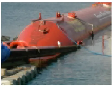
Nowadays, there is an increasing demand for renewable energy sources. In this context, the number of energy installations in the ocean, off-shore wind mills and wave energy farms will likely grow in the future. Fig. 1 shows a wave energy generator known as “pelamis”. Such power plants, composed by several generators, will produce considerable acoustic noise which propagates through the ocean, and will likely affect the oceanic environment and fauna to some extent[1], [2], [3]. In November 2007, the Wave Energy Acoustic Monitoring (WEAM) project was initiated, aiming at developing, testing and validating a monitoring system for determining underwater acoustic noise generated by wave generators, and their impact

Fig. 1. Wave energy converter Pelamis.

in the sea fauna. Another objective of this project is to develop a methodology to predict the noise distribution on a candidate area for installation of a wave energy farm. The development of such a methodology will give rise to tools that will allow the developer/engineering team in an early phase of the project to predict the influence of such an installation in the environment, or decide about the optimal configuration in order to mitigate it (“best practice” tool). An initial model of the noise distribution can be obtained by combining archival data, both hydrologic and geologic, with outputs from oceanographic and acoustic modeling tools. However, this initial acoustic noise model should be refined with actual measurements in the interest area, even in case a large archival data set is available. Although several approaches can be considered to minimize the modeling errors, for instance based on frequent sound speed profile measurements, bottom surveys and cores and more powerful modeling tools, they are costly, and herein, an alternative method is considerd. This alternative method, named (acoustic) field calibration, consists of integrating re-sults obtained from acoustic inversions for acoustic-sensitive parameters, like bathymetric and geoacoustic parameters, in the final acoustic noise distribution predictions. Since the goal is to accurately model the acoustic field, one could consider a method in which a ship would probe the area with acoustic signals, and measure the point-to-point transmission loss, to construct a map. Nevertheless, it would be necessary to do a prohibitively large survey in the three-dimensional ocean. Instead, and taking into account that there are environmental properties which do not change in time (e.g. geological prop-erties), the procedure here is to use remote acoustic sensing

to infer the values of these properties. Then, these values can be used in a laboratory, to predict the field for any source-receiver configuration required in the project. The idea is that the information about the environment, obtained by acoustic inversions, is sufficient and irreplaceable to attain an acoustic noise model for the area[4]. This idea has been used in the past, in the field of geology[5]. The field calibration method is a low cost method when compared with other methods which require detailed hydrological and seafloor surveys of the area of interest.

This paper is organized as follows. Next, the problem is formulated in mathematical terms. In sec. III, it is described the experimental setup of the sea trial. The inversion results, and subsequent noise prediction lying on the former, are presented in sec. IV, followed by the conclusions.

II. PROBLEM STATEMENT AND BACKGROUND

Let us consider an oceanic area, in which the acoustic field due to an acoustic source is to be predicted. Here, the concept of “prediction” should be understood as “modeling”, as opposed to the estimation of future quantities. In the context of the present work, the acoustic source represents a given wave energy generator, whose acoustic signature, in terms of signal power over frequency is known by the user, either from technical descriptions from the manufacturer, or from direct measures made in the past. The resultant acoustic field at a generic point P is a function of several environmental proper-ties, as well as the acoustic source and the point coordinates. Thus, we can write the acoustic field Y at P , at each frequency f , as:

Y (f ) = φf(θ0), (1)

where θ0 represents all the environmental and system (emit-ter/receiver) properties relevant to acoustic propagation. In the problem at hand, the objective is to estimate the field Y at any user-defined frequency f , in an area for which the properties θ0 are not known in full detail. The premise of the present work is that, if some acoustic observations X are taken in the same area, in a training phase, then, valuable information can be obtained, for example, about the time-invariant properties (bottom properties, bathymetry, etc.). That information can easily be included in the planning phase of a wave energy farm, in which the designer will do a series of acoustic forward modeling runs, varying the positions of the acoustic source and point P , thus having a complete map of the noise in the area, produced by the wave energy converter. Since the goal is to accurately model the acoustic field, the training phase consid-ered here consists of probing the area with acoustic signals, and estimating the environmental properties values that best model the observed fields. This is the concept of acoustic in-version, which has been largely studied since the 1970’s. Many works like the ones of Baggeroer[6], Collins[7], Gerstoft[8], Richardson[9], Jesus[10] and Elisseeff[11], showed successful results of environmental estimation using acoustic signals. These approaches, though having as target the estimation of

ET

EI

EP

X

Y

Fig. 2. Acoustic field dependencies on environmental properties EI

(time-invariant), and ET and EP (time-variant). The field measured for calibration

is represented by X, and the field to model, by Y.

the environment, are favorable to the objective at hand, since they optimize for the modeled acoustic field.

In the present approach, in schematic terms, it is assumed that the field samples observed in the ‘training phase’, X, are a function of the time-invariant properties EI and time-variant properties ET, and the field Y observed in the case that a source was placed in the area of interest, is also a function of EI, and the time-variant properties EP, at the time of the project phase —see fig. 2. The present approach can be structured as:

1) Use the acoustic field samples X, to estimate the prop-erties ET and EI;

2) Use the estimated properties to estimate the acoustic field Y.

The next section develops on the inversion methods used in step 1).

A. Acoustic inversion

As said previously, in the context of the CALCOM’10 sea trial, the training phase consisted of using acoustic field observations to estimate environmental properties. This task resorted to matched field processing, whose principle is to look for the environmental properties that, when fed to an acoustic propagation model, conduce to a simulated field very close to the observed one, in terms of spatial correlation. This procedure can be interpreted as a problem of acoustic signal detection, propagated in a medium with unknown properties. This is an optimization problem, in which a cost function — the processor— involving an acoustic field correlation, is to be maximized, as a function of the environmental properties. One of the popular matched-field processors is the broadband incoherent Bartlett processor, defined by:

PB(θ) = 1 K K X k=1 wH(fk, θ) ˆRXX(fk, θ0)w(fk, θ), (2) where w(θ), function of the candidate environment θ, is a vec-tor of (complex) acoustic pressures at an array of sensors, and

−130 −128 −128 −128 −126 −126 −126 −124 −124 −124 −124 −124 −122 −122 −122 −120 −120 −120 −118 −118 −118 −116 −116 −116 −114 −114 −114 −112 −112 −112 −110 −110 −110 Water depth [m] Longitude [°W] Latitude [ ° N] 8.038 8.036 8.034 8.032 8.03 8.028 8.026 36.865 36.87 36.875 36.88

Fig. 3. Bathymetry of the CALCOM’10 sea trial site, with the acoustic source (◦) and receivers (X) superimposed on. The start and end positions of the acoustic instrumentation is represented by the green and red colors, respectively.

ˆ

RXX(θ0) is an estimate of the hydrophone data correlation matrix at frequency fk.

III. EXPERIMENTAL RESULTS

A. The experimental setup

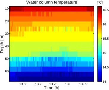
One of the objectives of the CALCOM’10 sea trial was to gather data to support the field calibration concept. The chosen area is in the continental shelf of the southern coast of Portugal, a prospective region to install wave energy farms in the future. The CALCOM’10 experiment took place off the southern coast of Portugal, about 12 nmi southeast of Vilamoura, from 22nd to 24th June 2010, in an area with the bathymetry shown in fig. 3. The data analyzed herein was acquired on 24th June along the continental steep slope to the deeper ocean, fig. 3. The source was towed, and the signals were acquired by an Acoustic Oceanographic Buoy (AOB)[12], from which 15 hydrophones were selected for analysis, deployed in a free drifting mode. The positioning information is given by the GPS installed in the buoy and on the boat. Pressure and temperature sensors were installed in the towfish to estimate the source depth and temperature. Fig. 4 shows the source depth recorded on 24th June. The field calibration signals analyzed here started at 1:36 PM and finished at 1:53 PM. The AOB has an array of 15 low resolution (0.5◦C) temperature sensors collocated with the hydrophones. Fig. 5 shows the temperature data acquired by the AOB during the considered period. For field calibration purposes, the transmitted probe signals transmitted included a 15-s long mixture of eleven tones (multitones) covering the 500–2000 Hz band. Those sequences were repeated in periods of 10–20 minutes, and are analyzed in the following. Figure 6 shows a spectrogram of an acoustic data sample (packet)

13.6 13.65 13.7 13.75 13.8 13.85 13.9 13.95 6.5 7 7.5 8 8.5 9 9.5 10 10.5 Time [h] Source depth [m]

Fig. 4. Source depth estimate from the water level sensor attached to the source towfish.

Time [h]

Depth [m]

Water column temperature

13.65 13.7 13.75 13.8 13.85 10 20 30 40 50 60 [°C] 14 14.5 15 15.5 16 16.5

Fig. 5. Water column temperature given by the AOB temperature sensors, between 10.3 and 66.3 m.

acquired on 24th June, at 1:36 PM, on the hydrophone at 6.3 m, at an approximate source-receiver range of 1.6 km. B. Data processing

The tones received in the AOB were processed, according to the processor in eq. (2). The matrix estimates in the processors were obtained with 10 data snapshots. The estimation of the source depth and source-receiver range was done with tight search intervals, to compensate for modeling/sensor errors. The search resorted to a continuous-variable genetic algorithm, with 2 populations running independently. The acoustic for-ward modeling was carried out with the BELLHOP Gaussian beam tracing model[13].

Time [s]

Frequency [Hz]

Spectrogram of received tones

2 4 6 8 10 12 14 400 600 800 1000 1200 1400 1600 1800 2000 Amplitude 0 20 40 60 80 100

Fig. 6. Spectrogram of the received tones acquired on 24th _{June, at 1:36}

PM, on the hydrophone at 6.3 m, at a approximate source-receiver range of 1.6 km.

IV. RESULTS

A. Acoustic inversion

The acoustic data inversion results are presented next, and the reader can refer to fig. 7, which shows the baseline and estimated values of the environmental model parameters. Prior to interpret the results in the figure, one has to take into account that the acoustic field is, in general, highly sensitive to changes in geometric parameters, moderately sensitive to changes in water column parameters, and moderately-to-weakly sensitive to changes in geoacoustic parameters. The figure shows time-varying results for all the estimates. For the deepest and shallowest sound speed value in the water column, this can indicate that the real values actually changed over the ≈ 30 min period. The parameter hydrophone array vertical shift is a nuisance parameter, useful to compensate for modeling errors (e.g. of not considering surface waves). The bottom compressional speed estimates suggest that the source insonified a medium with space-variant properties, over time. The bathymetry vertical shift suggests that it is necessary to subtract < 2 m to the prior bathymetry. As expected, the bottom density and compressional attenuation estimates are not stationary. Nevertheless, the range of values for the 3 bottom parameters suggest that the bottom, even if being a silty bottom as assumed, is more acoustically absorbing than expected.

The natural question is now to use the inversion results to construct an environmental model for the area. By assuming that the acoustic field realizations obtained over time are statistically independent, and by modeling the environmental parameters, except the source depth and source-receiver range as space-invariant, it is possible to obtain a posterior density of every parameter, conditioned on all the observed acoustic data, by multiplying the posterior densities corresponding to each

13.6 13.7167 13.8333

1450 1500 1550

Deepest sound speed value [m/s]

13.6 13.7167 13.8333

1500 1600 1700

Bottom compressional speed [m/s]

13.61 13.7167 13.8333 1.5 2 2.5 3 Bottom density [g/cm3 ] 13.60 13.7167 13.8333 1 2

Bottom compressional attenuation [dB/λ]

5 10 15 Time [h] Source depth [m] −2 0 2 Time [h]

Hydrophone array vertical shift [m]

0 1 2 Time [h] Source−receiver range [km] 1450 1500 1550 Time [h]

Shallowest sound speed value [m/s]

−2 0 2

Time [h]

Bathymetry vertical shift [m]

Fig. 7. Inversion results along time for the considered environmental parameters, using 11 tones in the band [500, 2000] Hz. The baseline and estimated values (maximum of the Bartlett cost in eq. (2)) are shown in green and blue colors, respectively.

14900 1500 1510 1520 0.5

1

Deepest sound speed value [m/s]

1520 1540 1560 1580 1600 0

0.5 1

Bottom compressional speed [m/s]

1.2 1.4 1.6 1.8 2 0 0.5 1 Bottom density [g/cm3_] 0.6 0.8 1 1.2 0 0.5 1

Bottom compressional attenuation [dB/λ]

−1 0 1

0 0.5 1

Hydrophone array vertical shift [m]

1514 1516 1518 1520

0 0.5 1

Shallowest sound speed value [m/s]

−1 −0.5 0 0.5 1

0 0.5 1

Bathymetry vertical shift [m]

Fig. 8. Marginal posterior densities for the estimated environmental param-eters, defined as the product of the posterior densities obtained for each of the 18 acoustic inversions.

TABLE I

BASELINE ANDBAYESIAN ESTIMATES OF THE ENVIRONMENTAL

PARAMETERS,EXCLUDING THE ACOUSTIC SYSTEM PARAMETERS

(SOURCE DEPTH AND SOURCE-RECEIVER RANGE).

Parameter Baseline MAP≡Median Mean

Deepest sound speed [m/s] 1508 1516 1513

Bottom comp. speed [m/s] 1575 1520 1528

Bottom density [g/cm3] 1.70 1.33 1.33

Bottom comp. att. [dB/λ] 1 0.797 0.797

Sensor array vertical shift [m] 0 1.14 1.14

Shallowest sound speed [m/s] 1514 1516 1516

Bathymetry vertical shift [m] 0 -0.376 -0.377

inversion. By proceeding this way, the obatined densities are as shown in fig. 8. The obtained marginal probability density functions are narrow, as a result of the redundancy on the observation of an assumed space- and time-variant area.

The definition of a single marginal density for every of the 7 parameters as in fig. 8 leads naturally to Bayesian estimates of the parameters, namely the maximum a posteriori (MAP), median and mean. These estimates are given in tab. I, along with their corresponding prior (baseline) values, where “comp.”, “att.” stand for “compressional” and “attenuation”, respectively. For the assumed discretizations, the MAP and median estimates coincide.

B. Noise prediction

The estimates obtained by acoustic inversion were used to compute acoustic fields, and these fields were compared to the observed ones, using the acoustic fit measure defined by the Bartlett processor in (2). The fit over time is shown in fig. 9. As we can see, in most of the 18 cases, the acoustic fit corresponding to environmental values coming from acoustic inversion is larger than the one corresponding to the baseline values. The exceptions correspond to the cases in which the instantaneous values shown in fig. 7 are more appropriate to model the field.

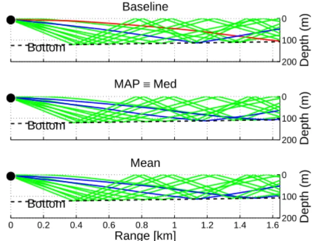
In terms of propagation paths, the gain of acoustic inversion can be seen in the ray tracing in fig. 10. The figure shows

13.6 13.65 13.7 13.75 13.8 13.85 13.9 0.1 0.2 0.3 0.4 Time [h] Acoustic fit Baseline Mean Median≡MAP

Fig. 9. Acoustic fit (Bartlett power, defined in (2)) corresponding to the baseline and estimated parameters.

0 100 200 _{Depth (m)} Baseline Bottom 0 100 200 _{Depth (m)} MAP ≡ Med Bottom 0 0.2 0.4 0.6 0.8 1 1.2 1.4 1.6 0 100 200 Range [km] Depth (m) Mean Bottom

Fig. 10. Gaussian beam tracing sample (11 Gaussian beams between -16 and 16◦) corresponding to the baseline environment and the ones estimated by acoustic inversion.

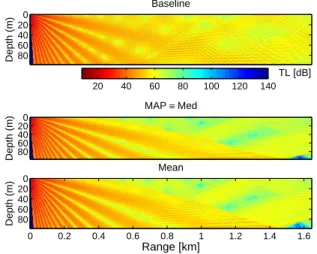
that the baseline parameter values lead to a water column which is more insonified near the surface, than the values obtained from inversion. This can be explained by a baseline lower shallowest sound speed of 1514 m/s, as opposed to 1516 m/s from inversion —see tab. I. Moreover, the larger baseline value for the bottom compressional speed leads to a smaller attenuation of acoustic energy at the water-bottom interface, and consequently to a less attenuated field over range from the acoustic source. These statements are illustrated with a plot of the acoustic transmission loss in fig. 11, corresponding to the ray tracing in fig. 10. Histograms of the differences between the transmission loss corresponding to the baseline parameters and the ones corresponding to the inverted ones were computed, and are shown in fig. 12. The median of the histograms is less than 5 dB, which is not a high value. Even though, this value was computed as a small distance from the source (< 2 km), and large values may be obtained at tens of km, due to cumulative effects, and being significant for the purposes at hand.

V. CONCLUSION

A noise prediction tool has been presented, which incorporates acoustic measures in the area of interest, acoustic inversion and acoustic forward modeling. Having as target the prediction of the noise generated by a wave energy converter, the present

Depth (m) Baseline 0 20 40 60 80 TL [dB] 20 40 60 80 100 120 140 Depth (m) MAP ≡ Med 0 20 40 60 80 Range [km] Depth (m) Mean 0 0.2 0.4 0.6 0.8 1 1.2 1.4 1.6 0 20 40 60 80

Fig. 11. Transmission losses corresponding to the baseline and estimated environmental parameters. 0 20 40 0 0.5 1 1.5 2 2.5 3 3.5 4x 10 −3 |Nominal − MAP| [dB] Frequency Median = 4.9 dB 0 20 40 0 0.5 1 1.5 2 2.5 3 3.5 4x 10 −3 |Nominal − Mean| [dB] Frequency Median = 4.4 dB

Fig. 12. Histograms of the differences between the transmission loss field corresponding to the baseline parameter values, and the transmission losses corresponding to each of the estimates, shown in fig. 11.

work described the prediction tool, giving emphasis to the acoustic inversion phase. The inverted data was acquired in the CALCOM’10 sea trial, in Portugal, in 2010, and allowed to construct an environmental model for a prospective area of wave energy farms. The inversions used medium-high frequency signals in the band 500–2000 Hz, and were carried for 18 data packets during ≈ 30 min. The construction of probability densities for the estimated parameters, conditioned in all the acoustic data, allowed the parametrization of the oceanic area with a single environmental vector. The com-parison of synthetic fields generated with this environmental vector, to the measured ones, shows promising results in terms of field calibration.

Future work will include the definition of space or time domains of validity of the obtained environmental parameters, and/or the definition of sampling needs in a field calibration experiment.

ACKNOWLEDGMENT

This work was partially supported by FCT, Portugal (ISR/IST plurianual funding), through the PIDDAC Program funds, through project FCT WEAM (PTDC/ENR/70452/2006) and through the scholarship FCT SFRH/BD/9032/2002.

REFERENCES

[1] J. Tougaard, O. D. Henriksen, and L. A. Miller, “Underwater noise from three types of offshore wind turbines: Estimation of impact zones for harbor porpoises and harbor seals,” J. Acoust. Soc. Am. , vol. 125, no. 6, pp. 3766–3773, 2009.

[2] J. Nedwell, A. Turnpenny, J. Langworthy, and B. Edwards, “Measure-ments of underwater noise during piling at the red funnel terminal, southampton, and observations of its effect on caged fish,” Subacoustech Ltd, Tech. Rep. 558 R 0207, October 2003.

[3] J. Nedwell, J. Langworthy, and D. Howell, “Assessment of sub-sea acoustic noise and vibration from offshore wind turbines and its impact on marine wildlife; initial measurements of underwater noise during construction of offshore windfarms, and comparison with background noise,” Subacoustech Ltd, Tech. Rep. 544 R 0424, May 2003. [4] N. Martins, C. Soares, and S. Jesus, “Environmental and acoustic

assessment: The aob concept,” Journal of Marine Systems, vol. 69, pp. 114–125, 2008.

[5] William A. Jury and Garrison Sposito, “Field calibration and validation of solute transport models for the unsaturated zone,” Soil Sci. Soc. Am. J., vol. 49, no. 6, pp. 1331–1341, November 1985. [Online]. Available: https://www.soils.org/publications/sssaj/abstracts/49/6/1331

[6] A. Baggeroer, W. Kuperman, and H. Schmidt, “Matched-field process-ing: Source localization in correlated noise as an optimum parameter estimation problem,” J. Acoust. Soc. Am. , vol. 80, pp. 571–587, 1988. [7] M. Collins and W. Kuperman, “Focalization: Environmental focusing and source localization,” J. Acoust. Soc. Am. , vol. 90, pp. 1410–1422, 1991.

[8] P. Gerstoft, “Inversion of acoustic data using a combination of genetic algorithms and the gauss-newton approach,” J. Acoust. Soc. Am. , vol. 97, pp. 2181–2190, 1995.

[9] A. Richardson and L. Nolte, “A posteriori probability source localization in an uncertain sound speed deep ocean environment,” J. Acoust. Soc. Am., vol. 89, pp. 2280–2284, 1991.

[10] S. Jesus, “Normal-mode matching localization in shallow water: environ-mental and system effects,” J. Acoust. Soc. Am. , vol. 90, pp. 2034–2041, 1991.

[11] P. Elisseeff, H. Schmidt, M. Johnson, D. Herold, N.R. Chapman, and M.M. McDonald, “Acoustic tomography of a coastal front in Haro Strait, British Columbia,” J. Acoust. Soc. Am. , vol. 106, No. 1, pp. 169–184, 1999.

[12] A. Silva, F. Zabel, and C. Martins, “Acoustic oceanographic buoy: a telemetry system that meets rapid environmental assessment require-ments,” Sea Technology, vol. 47, no. 9, pp. 15–20, 2006.

[13] M. Porter and H. Bucker, “Gaussian beam tracing for computing ocean acoustic fields,” J. Acoust. Soc. Am. , vol. 82, no. 4, pp. 1349–1359, 1987.