UNIVERSIDADE DE LISBOA
FACULDADE DE CIÊNCIAS
DEPARTAMENTO DE GEOLOGIA
Factors impacting multi-layer plume distribution in CO2 storage
reservoirs
Andrea Callioli Santi
Mestrado em Geologia
Especialização em Estratigrafia, Sedimentologia e Paleontologia
Dissertação orientada por:
Professor Doutor Nuno Lamas de Almeida Pimentel
Dr. Philip Ringrose, Equinor Energy AS, Norway
Acknowledgements
First of all I wish to express my deepest gratitude to Philip Ringrose for the incredible opportunity of developing a master’s thesis with Equinor in such an exciting topic and the valuable guidance and support throughout this year.
I would like to thank the Sleipner CO2 storage team in Equinor Anne-Kari Furre, Peter Zweigel, Bamshad Nazarian and Britta Paasch for the expert insights and interesting discussions. Grethe Tangen and Odd Andersen from SINTEF for the feedback and support of the modelling work performed on this project.
I am grateful to Professor Nuno Pimentel for the technical inputs and guidance in developing this master’s thesis with the Department of Geology of the Faculty of Science of the University of Lisbon from Norway.
Thanks to Equinor Energy AS and the Sleipner partnership for the dataset and permission to publish this material. Also to Halliburton for granting an academic license for the Permedia CO2 toolkit software for the development of this thesis.
Abstract
The Sleipner Carbon Capture and Storage project in the North Sea has been injecting CO2 underground into a saline formation for permanent storage for over 22 years. Equinor Energy AS, the field operator, and the license partners have injected about 18 million metric tons (Mt) of CO2 by the end of 2018 into the Utsira Formation at depths around 800 to 1100 m below sea level.
The Sleipner CO2 storage reservoir comprises mostly unconsolidated sands with high porosities (36%) and high permeabilities (Darcy range) under near hydrostatic pressure conditions. An intensive geophysical monitoring program has been implemented since CO2 injection commenced in 1996. Nine bright reflections were already identified in the first time-lapse repeat survey in 1999 indicating that the CO2 ascended more than 200m vertically from the injection point to the caprock. The CO2 plume is evidently layered and asymmetric with a vertical stack distribution indicating that it encountered and breached a series of thin shale barriers (about 1m thick) within the storage site. The thin shale layers within the Utsira Formation acting as baffles to the CO2 migration were identified on well data but too thin to be resolved on seismic. Core and cutting samples of the caprock above the storage reservoir have indicated threshold pressures around 1.7 MPa. In order for the CO2 to break through the shale layers within the reservoir and form a vertical stack of thin plume layers, their threshold pressures need to be significantly smaller than the sampled caprock.
Despite the high quality time-lapse seismic surveys imaging of the areal distribution of the CO2 plume in Sleipner, to date no published dynamic model has accurately replicated the layered morphology or flow behaviour of the plume. This is due to challenges around the underlying flow physics of CO2 and uncertainties in geological assumptions. Equinor has previously released benchmark reservoir models of Sleipner focusing on the uppermost plume layer (Singh et al., 2010). This master’s thesis objective was to define the full Sleipner multi-layer reservoir model in order to analyse the key factors controlling gravity-dominated flow in CO2 storage reservoirs, based on assumptions from Cavanagh et al. (2015).
Fundamental aspects of the plume remain uncertain such as layer thickness, plume temperature profile (which impacts CO2 densities) and gas saturations for the plume layers. These uncertainties are inherited from the remote geophysical monitoring of the CO2 storage reservoir and the broadly constrained fields of pressure, temperature and saturation (Cavanagh and Haszeldine, 2014).
Two main reservoir models were built in the Permedia software for the Sleipner CO2 storage in this study, a simple and a map-based approaches. The simple approach defined constant values for the reservoir properties and the map-based assigned lateral distributions to the reservoir properties corresponding to the areal distribution of the CO2 layers observed in seismic. Invasion percolation was applied to simulate the CO2 migration which assumes a flow domain dominated by gravity and capillary forces over viscous forces, similar to the expected in Sleipner.
Using iterative experimentation in an Invasion Percolation (Permedia tool) simulator, values of shale threshold pressure (Pth) were modified until a satisfactory match was achieved.It was established that the multi-layer plume was very sensitive to the choice of Pth and the best match was obtained by using lower threshold pressures which could indicate pore sizes associated with silt-rich shales. A sensitivity analysis of the poorly constrained parameters, temperature (and related CO2 densities) and gas saturations, was performed to assess their impact on the CO2 migration simulation. Other models are also possible, such as incorporation of chimneys (leakage points), which need to be investigated in future studies.
Key-words: Geological carbon storage; Sleipner; invasion percolation simulation; threshold pressures; multi-layered CO2 plume.
Resumo
A captura e armazenamento geológico de dióxido de carbono é considerada uma solução essencial para atingir os objetivos do Acordo de Paris sobre as alterações climáticas, visando manter o aumento da temperatura média mundial bem abaixo dos 2℃ em relação aos níveis pré-industriais. De acordo com a International Energy Agency (IEA), a captura e armazenamento de carbono – CCS (sigla em inglês para Carbon Capture and Storage) é a única tecnologia com capacidade para reduzir as emissões de CO2 em larga escala, necessária para alcançar os objetivos de longo prazo na mitigação do aquecimento global. O CCS consiste na captura de CO2 de grandes fontes estacionárias, como centrais termo-elétricas e instalações industriais, seguida de sua compressão, transporte por gasodutos ou navios e injeção para armazenamento geológico em formações rochosas com alta porosidade.
O campo de Sleipner está localizado a cerca de 250 km da costa da Noruega, na parte central do Mar do Norte. O projeto de captura e armazenamento é combinado com o desenvolvimento e produção deste campo de gás. O campo é dividido em Sleipner Oeste e Leste, sendo que a produção do Sleipner Oeste apresenta conteúdos altos de CO2 para o mercado consumidor. O CO2 é entretanto separado e injetado numa grande formação salina localizada acima do campo Sleipner Leste, a cerca de 800 metros abaixo do fundo oceânico. O CO2 tem sido injetado para armazenamento permanente por mais de 22 anos em Sleipner, sendo este o primeiro projeto de captura e armazenamento de CO2 em larga escala no mundo. A Equinor Energy AS, empresa operadora, e empresas parceiras injetaram na Formação Utsira (depósitos marinhos do Miocénico) cerca de 18 milhões de toneladas métricas (Mt) de CO2 até ao final de 2018. A sequência de lutitos (shales) do Grupo Nordland depositada acima da Formação Utsira foi comprovada como uma rocha selante efetiva para o reservatório de armazenamento de CO2 (Singh et al., 2010).
O reservatório Sleipner de armazenamento de CO2 é composto principalmente por arenitos mal consolidados com excelentes propriedades - porosidades em torno de 36% e permeabilidades em torno de 1 a 5 Darcy. Este reservatório está sob condições de pressão próximas a hidrostáticas, com salinidade das águas intra-formacionais com valores similares aos da água do mar. Desde o início do projeto em 1996, um programa intensivo de monitorização geofísica foi implementado. O Sleipner foi monitorizado com levantamentos geofísicos aproximadamente a cada 2 anos, o que permitiu a delineação de uma imagem detalhada da distribuição e dinâmica da pluma de CO2. No primeiro levantamento sísmico 4D (time-lapse seismic) em 1999, apenas 3 anos após o início da injeção, foram identificados 9 refletores com fortes contrastes de impedância acústica (bright reflectors), o que indica que o CO2 ascendeu verticalmente mais de 200 metros, do ponto de injeção até a rocha selante (caprock). A distribuição vertical da pluma de CO2 é evidentemente assimétrica e em camadas, indicativa do encontro e migração através de uma série de finas barreiras de shales (com cerca de 1 metro de espessura) dentro do reservatório. Estas finas camadas de shales que agiram como barreiras semi-permeáveis (baffles) à migração de CO2 foram identificadas em dados de poço mas, com exceção da unidade Thick Shale (com cerca de 6.5 metros de espessura) que separa a Formação Utsira da unidade arenosa Sand Wedge localizada logo abaixo da rocha selante, não foi possível realizar uma correlação devido às grandes distâncias entre os poços nem identificá-los na sísmica devido à resolução. Estima-se que cada camada de CO2 apresentará espessuras entre 7 e 20 metros, com extensão lateral de 1 a 3 quilómetros (Cavanagh et al., 2015). Cada camada de CO2 apresenta um pronunciado
alongamento na direção norte-sul, indicativo da forte influência da topografia da rocha selante e da unidade Thick Shale.
A migração vertical do CO2 é resultante do grande contraste entre as densidades da água (presente nos poros da formação rochosa, brine) e do CO2. Quando o CO2 atinge uma barreira com rochas de baixa permeabilidade, ele acumula-se abaixo desta barreira, com o preenchimento de pequenas armadilhas ou estruturas (traps) em conformidade com sua topografia. O CO2 migra através destas barreias de baixa permeabilidade quando a pressão exercida pelo fluido de CO2 supera a pressão limite para invasão do CO2 (threshold ou displacement pressures) da rocha de baixa permeabilidade. Amostras de testemunho e cuttings da rocha selante (caprock) acima do reservatório indicaram pressões limite para invasão do CO2 de cerca de 1.7 MPa. Para o CO2 conseguir migrar através das camadas de shales do reservatório e formar uma pluma composta por um empilhamento vertical de camadas finas, as pressões limite para invasão do CO2 precisam de ser significativamente menores que o valor indicado pelas amostras da rocha selante.
Apesar da alta qualidade das imagens da distribuição espacial da pluma de CO2 em Sleipner, adquiridas por levantamentos sísmicos 4D, até hoje nenhum modelo dinâmico publicado reproduziu com sucesso a morfologia em camadas ou o comportamento do fluxo da pluma de CO2. Isto é devido aos desafios relacionados com a física inerente aos fluxos de CO2 e às incertezas relacionadas com as interpretações geológicas. A Equinor publicou anteriormente modelos do reservatório Sleipner de armazenamento de CO2, para referência da comunidade científica, com foco na camada superior da pluma, uma vez que as interpretações das estruturas correspondentes ao topo do reservatório foram realizadas no levantamento sísmico 3D, com menos incertezas relacionadas com os efeitos do CO2 (Singh et al., 2010). A presente Tese de Mestrado definiu o modelo do reservatório completo com a incorporação das 9 camadas de CO2 para analisar os fatores principais que controlam o fluxo dominado por gravidade em reservatórios de armazenamento de CO2, com base em suposições de acordo com Cavanagh et al. (2015).
Alguns aspectos fundamentais da pluma permanecem incertos, tais como a espessura das camadas (dependentes das pressões limite para invasão do CO2 das unidades shale), o perfil de temperatura da pluma (o qual impacta as densidades do CO2) e a saturação em gás das camadas da pluma (parâmetro difícil de distinguir acima de 30%). Estas incertezas são devidas às características intrínsecas da monitorização sísmica remota e da ampla variação possível dos parâmetros pressão, temperatura e saturação num reservatório (Cavanagh & Haszeldine, 2014).
O desenvolvimento desta Tese de Mestrado incorporou a construção de dois modelos principais do reservatório de CO2 Sleipner no software Permedia, um com uma abordagem simples e o outro baseado em mapas. A abordagem simples consistiu na definição de valores constantes para as propriedades do reservatório, enquanto a abordagem por mapas definiu distribuições laterais para as propriedades das rochas do reservatório conforme a distribuição espacial das camadas de CO2 observada em sísmica com significativo alongamento norte-sul. O método de percolação por invasão (invasion percolation) foi aplicado para simular a migração de CO2, o qual assume um fluxo dominado pelas forças da gravidade e da capilaridade sobre a viscosidade, de modo similar ao processo interpretado para o reservatório Sleipner.
As pressões limite para invasão do CO2 (threshold ou displacement pressures) foram estimadas por experimentação, através da sistemática redução do valor medido nas amostras da rocha selante até que a distribuição das 9 camadas de CO2 empilhadas verticalmente fosse reproduzida. As pressões limite para invasão do CO2 (threshold ou displacement pressures) efetivas para as unidades intra-shales e as correspondentes permeabilidades indicaram que seus valores reduzidos poderiam ser devidos a uma maior dimensão da generalidade das gargantas dos poros (pore throat sizes), associada à presença de shales mais ricas em silte. Uma análise de sensibilidade dos parâmetros com alta incerteza - temperatura (e consequentes
densidades de CO2) e saturações do CO2 - foi realizada para avaliar os seus impactos na migração de CO2 e identificar os fatores-chave que contribuem para a distribuição da pluma de CO2 em múltiplas camadas. Estudos futuros devem investigar outros modelos possíveis, especialmente com a incorporação de áreas com alta permeabilidade interpretadas como “chaminés” (chimneys, leakage points) em sísmica.
Contents Acknowledgements ... i Abstract ... ii Resumo ... iii Figures ... vii I. Introduction ... 1
1. Why CO2 storage? ... 1
2. Project Scope and Objectives ... 3
3. Field Location and History ... 4
II. Geological Framework and CO2 Storage ... 6
1. Regional Geology ... 6
1.1. South Viking Graben ... 6
1.2. Utsira Formation ... 8
2. Sleipner CO2 Storage ... 9
2.1. Storage Reservoir ... 9
2.2. Observed CO2 Plume Distribution ... 11
3. CO2 Flow Dynamics ... 14
3.1. CO2 Storage Flow Dynamics ... 14
3.2. Sleipner CO2 Flow Behaviour ... 16
III. Dataset ... 17 1. Seismic Data ... 18 2. Well Data ... 20 2.1. Reservoir Properties ... 20 2.2. Fluid Properties ... 22 2.3. Injected volumes ... 22
2.4. Previous Sleipner Benchmark Models ... 23
IV. Modelling Methodology ... 24
1. Geological Controls on CO2 Migration ... 24
2. Conceptual Model ... 27
3. Geomodel Grid Design ... 29
4. Property Modelling ... 31
5. CO2 Migration Simulation ... 36
1. Reservoir Modelling Approaches ... 39
2. Plume Temperature Scenarios ... 42
3. CO2 Saturations Scenarios ... 44
VI. Analysis and Discussion ... 47
1. Reservoir Modelling Approaches ... 47
2. Plume Temperature Scenarios ... 53
3. CO2 Saturations Scenarios ... 54
VII. Conclusions ... 56
VIII. References ... 57
Appendix 1 – Input Parameters (SPE 134891) ... 62
Figures Figure 1- Global CO2 emissions from 1800 to 2014 from combustion of fossil fuel, cement manufacture, gas flaring and global population (Sources: carbon emissions data from cdiac.ornl.gov, with years 2012 – 2014 based on data from BP statistical review; population data from www.census.gov In Ringrose, 2017). To convert the CO2 emissions from million metric tonnes of carbon to mass of CO2 multiply by the molecular ratio 3.667. ... 1
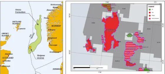
Figure 2– Left: Location map showing areal extent of the Utsira Formation and the Sleipner licence. Right: Sleipner field (West/Vest and East/Øst) license – PL046, block 15/9 (courtesy of the Norwegian Petroleum Directorate - NPD). ... 5
Figure 3- Simplified diagram of the Sleipner CO2 Storage Project (IPCC, 2005). CO2 is removed from the well stream at Sleipner T and injected into the Utsira Formation via a dedicated injection well (15/9-A-16) at Sleipner A facility. ... 5
Figure 4 - Regional structure map of the northern North Sea and Norwegian continental margin, with the outline of Sleipner field (modified from Kennett, 2008). ... 6
Figure 5- Stratigraphic correlation chart for the Cenozoic Hordaland and Nordland Groups. Sequence stratigraphic schemes: NNS = Northern North Sea; ENS = Eastern North Sea; CNS = Central North Sea (Fyfe et al., 2003). ... 7
Figure 6– Regional 2D seismic line across the North Sea basin showing the Utsira Sand and the caprock succession. Vertical yellow lines represent well-bore profiles, and the vertical blue lines represent gamma-ray well-log traces (Hermanrud et al., 2010). ... 8
Figure 7 – Left: Two-way travel time structure map to Top Utsira Sand. Right: Utsira Sand isopach map, showing the two main depocentres. CO2 injection well 15/9-A-16 displayed on both maps (Kirby et al., 2001 In Kennett, 2008). ... 9
Figure 8 – Gamma ray and sonic wireline log response through the Utsira Formation and the caprock shale. Reservoir characterized by the Sand Wedge, the Thick Shale and the main Utsira Sand units (modified from Kennett, 2008). ... 10
Figure 9 – Vertical seismic sections across the reservoir representing the 1994 baseline and the CO2 plume growth differences in 2001 and 2008, respectively (courtesy of Equinor). ... 12
Figure 10 – CO2 plume in map view based on time-lapse seismic difference reflection amplitude maps, cumulative for all layers. Expansion of the plume in all directions is observed, as well as intensified reflections in the central part of the plume (Eiken et al., 2011). ... 13
Figure 11 – CO2 layers lateral expansion as a function of time up to 2008, layers 1 to 9 from base to top of the reservoir. Warmer and colder colour show stronger and weaker amplitudes, respectively; solid black dot shows injection point (Boait et al., 2012). ... 14
Figure 12 – Effectiveness of geological storage in a saline formation increase with time as the physically trapped CO2 plume reacts with to brine becoming more immobile until it gets converted to solid minerals (IPCC, 2005). ... 16
Figure 13 – Illustration of the dynamics of CO2 storage. The injected CO2 will migrate upwards due to buoyancy and eventually fill a structural trap. Some residual trapping of CO2 may be left behind the migrating plume. There will be some convective mixing of CO2 with brine resulting in dissolved phase trapping of CO2 (Ringrose, 2018). ... 16
Figure 14 – CO2 phase behavior for the Sleipner storage reservoir (WH=Well Head, BH= Bottom-hole) and at surface (vapour around 20 degrees and 1 bar). The injected CO2 is very close to the critical point but still in the dense phase (modified from Eiken et al., 2011). ... 17
Figure 15 – Top Utsira TWT and wells in the area. Yellow rectangle shows the coverage of the released seismic data and yellow circle is the location of the injection point (well 15/9-A-16) (courtesy of Equinor). ... 18 Figure 16 – Top: Baseline seismic survey N-S section (1994) - blue reflector corresponds to an increase in acoustic impedance, and a red reflector corresponds to a decrease. Projection of the injection well path 15/9-A-16 (black line). ... . 19
Figure 17 – Depth converted surfaces provided for this thesis. From left to right: Top Sand Wedge, Top Utsira Formation, Base Utsira Formation. Colors scale get warmer with increase in depth. Injector well 15/9-A-16 is displayed and injection point (red circle). ... 19
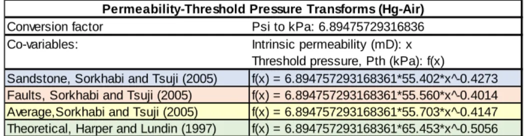
Figure 18 – Permeability-Threshold Pressure Transforms (Hg-Air system) based on Sorkhabi and Tsuji (2005) and Harper and Lundin (1997). ... 21
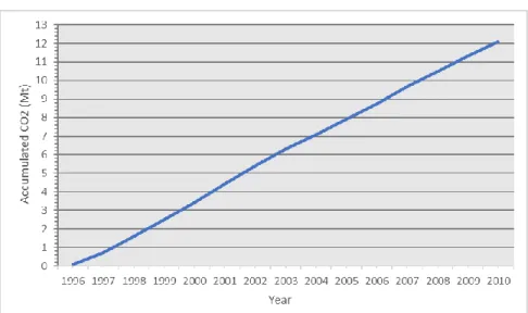
Figure 19 – Cumulative distribution of injected CO2 into Sleipner from 1996 to 2010. ... 23 Figure 20 – Pressure acting on top of an accumulation against a seal (ℎ =column height). The column pressure (buoyancy pressure or capillary pressure of the invading phase) must exceed the capillary pressure of the seal in order for breakthrough to occur (Hantschel and Kauerauf, 2009). ... 25
Figure 21 – Pore scale capillary trapping. The density contrast between CO2 and brine drives CO2 upwards through the reservoir (large pore throats) and it accumulates underneath rocks with small pore throats (high capillary entry pressures) (Hermanrud et al., 2009). ... 25
Figure 22 – Permeability-Threshold Pressure Transforms in Hg-Air system based on Sorkhabi and Tsuji (2005) and Harper and Lundin (1997) converted to the CO2-brine system of the Sleipner reservoir. ... 27
Figure 23 – Input data observed in 3D view in the Permedia software (VE= vertical exaggeration). High resolution input seismic surfaces Top Sand Wedge L9, Top Utsira Formation L8 and Base Utsira Formation, injector well 15/9-A16 and injection point. ... 29
Figure 24 - The intrashales depths within the Utsira Formation were estimated based on the cross-section provided by Cavanagh et al. (2015) and calculated conforming to the Top L8 structure depth. ... 30
Figure 25 – Geomodel grid design 3D view (left) and cross-section (right). (a) Nine reservoir zones divided by laterally continuous shale barriers. (b) Three-dimensional grid with cell dimensions 50mx50mx0.5m. ... 31
Figure 26 – Permeability-Threshold Pressure Average Transform in Hg-Air (yellow) and CO2-brine system (blue) for caprock input values. ... 32
Figure 27 – Map-based approach for Sand Wedge (L9). I. Isochore map from Williams and Chadwick (2017) with red polygon outlining the 20m isochore. II. Isochore map for the Sand Wedge L9 interval based on current input seismic depth surfaces. III. Permeability map with 8 D within thickness > 24m (red) and 3 D outside (blue). ... 33
Figure 28 – Map-based approach for the Sand Wedge (L9) unit – property maps created from the isochore (porosity, horizontal permeability and threshold pressure). ... 33
Figure 29 – Map-based approach for the Utsira Formation unit. Left: Top Utsira Formation seismic structure used to define a polygon trend. Right: Map created from polygon with high porosity and permeability zone (red) and lower outside (blue). ... 34
Figure 30 – Map-based approach for the Utsira Formation unit – property maps created from the isochore (porosity, horizontal permeability and threshold pressure). ... 34
Figure 31 - Map-based approach for the intrashales and caprock. Left: Porosity distribution map and histogram for the intrashales and caprock. Middle: Threshold pressures distribution map and histogram for the intrashales L1-L4 and L6-L8. Right: Threshold pressures distribution map and histogram for the intrashale L5. ... 35
Figure 32 - Map-based approach for the caprock. Threshold pressures distribution map and histogram for the caprock. ... 36
Figure 33 – CO2 dashboard generated graphs considering the Sleipner storage environment inputs... 37 Figure 34 - CO2 dashboard generated graphs considering the Sleipner storage environment inputs for the cold plume scenario (31˚C at the reservoir top as observed on the Geothermal Profile graph on the top left). ... 38
Figure 35 - CO2 dashboard generated graphs considering the Sleipner storage environment inputs for the warm plume scenario (37˚C at the reservoir top as observed on the Geothermal Profile graph on the top left). ... 38
Figure 36 - Simple approach migration simulation results in 2010 (12.08 Mt). (a) and (b) CO2 plume distribution in 3D view (vertical exaggeration 10x). (c) CO2 mass accumulated per layer. ... 40
Figure 37 - Map-based approach Pthz property for the intrashales, Utsira Sand (US) and Sand Wedge (SW). ... 41
Figure 38 - Map-based approach migration simulation results in 2010 (12.08 Mt). (a) and (b) CO2 plume distribution in 3D view (vertical exaggeration 10x). (c) CO2 mass accumulated per layer. ... 42
Figure 39 - Cold plume scenario migration simulation results in 2010 (12.08 Mt). (a) and (b) CO2 plume distribution in 3D view (vertical exaggeration 10x). (c) CO2 mass accumulated per layer. ... 43
Figure 40 - Warm plume scenario migration simulation results in 2010 (12.08 Mt). (a) and (b) CO2 plume distribution in 3D view (vertical exaggeration 10x). (c) CO2 mass accumulated per layer. ... 44
Figure 41 - Saturations sensitivity scenario 1 (SC1) migration simulation results in 2010 (12.08 Mt). (a) and (b) CO2 plume distribution in 3D view (vertical exaggeration 10x). (c) CO2 mass accumulated per layer. ... 45 Figure 42 - Saturations sensitivity scenario 2 (SC2) migration simulation results in 2010 (12.08 Mt). (a) and (b) CO2 plume distribution in 3D view (vertical exaggeration 10x). (c) CO2 mass accumulated per layer. ... 46
Figure 43 - Saturations sensitivity scenario 3 (SC3) migration simulation results in 2010 (12.08 Mt). (a) and (b) CO2 plume distribution in 3D view (vertical exaggeration 10x). (c) CO2 mass accumulated per layer. ... 47 Figure 44 - CO2 mass accumulated per layer (in kg) per year for the simple approach (note that X axis scale varies with the total CO2 accumulated mass injected). ... 49
Figure 45- CO2 mass accumulated per layer (in kg) per year for the map-based approach (note that X axis scale varies with the total CO2 accumulated mass injected). ... 49
Figure 46 - CO2 Mass accumulation (kg) per layer for the Simple (blue) and the Map-based (orange) approaches (2010, 12.08 Mt). ... 50
Figure 47 – Effective ranges for intrashales threshold pressures and their corresponding permeabilities based on the Pth-K Average Transform for the modelled results and Cavanagh et al. (2015) in Hg-Air and CO2-brine systems. ... 50
Figure 48 – Permeability anisotropy approximation for different lithologies (from Permedia). ... 51 Figure 49 - Horizontal to vertical permeability ratios (kh/kv) at 60 MPa effective stress per sample with grain sizes from fine silt to muddy siltstone. Sample 17 shows an extreme ratio of ~50,000 which is attributed to greater mineralogical layering (Armitage et al., 2011). ... 52
Figure 50- Grain size distribution measured on the caprock core samples (Springer and Lindgren, 2006). ... 53 Figure 51 - Comparison of density variation per layer (L9 at the top – 8123 MPa) for the warm and cold scenarios and the reference case. ... 53
Figure 52 - Comparison between the total CO2 mass accumulated and total column height for the uppermost layer L9 for the warm and cold scenarios and the reference case (top plot). Uppermost CO2 layer L9 density variation with temperature (bottom plot). ... 54
Figure 53 - Comparison between the reference case (CO2 saturation 89%, blue) and SC1 (CO2 saturation 40%, green) per layer for the same injected CO2 mass of 12.08 Mt (2010). ... 55
Figure 54 - Total CO2 volume comparison between reference case (critical CO2 saturation 2%, blue) and SC2 (critical CO2 saturation 20%, yellow) for the uppermost CO2 layer L9. ... 55
Figure 55 - Total CO2 volume accumulated per layer for the 3 saturation scenarios and the reference case. ... 56
I. Introduction
1. Why CO2 storage?
It is a worldwide consensus that reduction in global greenhouse gas emissions is crucial for the sustainable development of modern human civilization (Ringrose, 2017). The consumption of fossil fuels started with the industrial revolution in the beginning of the 19th century and rapidly increased after 1950 (Figure 1), resulting in substantial emissions of carbon dioxide (CO2). High rates of CO2 emissions to the atmosphere is a well-known significant contributor to global warming and ocean acidification (Cavanagh and Haszeldine, 2014).
Economic development of human society has been driven by energy from fossil fuels with current global fossil fuel consumption around 82% of the world energy supply according to the International Energy Agency (IEA, 2016a In Ringrose,2017). Considering that two-thirds of the current greenhouse gas emissions come from the energy sector, a transition to low-carbon energy systems is therefore an urgent priority.
Figure 1 - Global CO2 emissions from 1800 to 2014 from combustion of fossil fuel, cement manufacture, gas flaring and global population (Sources: carbon emissions data from cdiac.ornl.gov, with years 2012 – 2014 based on data from BP statistical
review; population data from www.census.gov In Ringrose, 2017). To convert the CO2 emissions from million metric tonnes of carbon to mass of CO2 multiply by the molecular ratio 3.667.
Carbon Capture and Storage (CCS) is a technology proposed by the G8 and the International Energy Agency as an essential solution to reduce CO2 emissions in order to mitigate climate change (Cavanagh and Haszeldine, 2014). It consists on the capture of CO2 from large stationary sources (power stations, industrial plants) which is then compressed, transported by pipeline or ships and injected for geological storage into porous rock formations deep below the land or sea surface (Cavanagh and Haszeldine, 2014). Saline aquifers and depleted oil and gas fields are considered the most viable injection targets (Bandilla et al., 2014). Deployment of CCS with CO2 used for enhanced oil recovery (EOR) is also an important option for large scale storage given the potential benefit of increased revenues (Senior et al., 2010). CCS technology has been largely applied to remove CO2 from natural gas processing, coal-fired power plants, as well as ethanol, fertilizer and hydrogen production plants (Ringrose, 2017). It is now also emerging as a primary mean to
decarbonize industrial processes, especially cement and steel manufactures. In addition, when combined with biomass-fired power plants it provides a major pathway into negative emissions (GCCSI, 2017).
The Paris Agreement limits the increase in global average temperature to well below 2°C above pre-industrial levels. The European Union has called for CO2 emissions reductions of 80% below 1990 levels by 2050, which is equivalent to 80 Gt (metric gigaton) of CO2 being kept out of the atmosphere. In order to reach this target, a transition into a low-carbon energy system will be required which consists of a combination of renewables, increased efficiency and Carbon Capture and Storage. CCS alone is expected to account for 12.2 Gt of CO2 emissions avoided by 2050, which implies average injection rates of 400 Mt/year (Gasda et al., 2016).
There are currently 18 large-scale CCS projects in operation worldwide with a collected capacity to capture and store about 32 Mtpa (million metric tonnes per annum) of CO2 according to the Global CCS Institute project database (https://www.globalccsinstitute.com/projects/large-scale-ccs-projects). This capacity should increase to 100 Mtpa by 2030, taking into account the CCS projects currently in the planning stages. This is still way beyond what would be required in order to meet the large-scale greenhouse reduction goal set by the Paris Agreement. Therefore, strategies to scale up CCS deployment have an urgency in development by governments, policy makers and private sectors (Ringrose et al., 2017).
The Sleipner Carbon Capture and Storage project in the North Sea was the first commercial CO2 storage site in the world. CO2 has been captured from the produced gas and re-injected it into an underlying saline formation since 1996. Equinor (formerly Statoil), the field operator, and Sleipner partners have injected about 18 million metric tons (Mt) of CO2 by the end of 2018 into the Utsira Formation, a Miocene aged shallow marine sandstone formation, at a depth of 800-1100 m below sea level in the Sleipner area. Overlying the sandstones is the Nordland Group shale sequence that has proven to be an effective seal for the CO2 storage site (Singh et al., 2010).
Sleipner has been monitored with geophysical surveys approximately every 2 years as well as gravimetric and electromagnetic surveys, defining a detailed image of the CO2 plume distribution and dynamics (Cavanagh, 2013). From 1996 to 1999, the CO2 plume ascended more than 200 m vertically from the injection point, breaching a series of thin shale barriers within the storage site, forming nine vertically stacked CO2 layers, each estimated about 7-20 m thick and extending laterally for a few hundred meters (Cavanagh et al., 2015). These intraformational shales within the main Utsira Sand unit are too thin to be resolved seismically (about 1 m thick) except for the uppermost barrier about 6.5 m thick. This thick shale barrier is overlain by a shallower sand unit beneath the caprock. Each CO2 layer has a pronounced north-south elongation appearing to be strongly influenced by the mapped topography of the caprock and underlying thick shale barrier, in a similar manner to the flat oil-water contacts of many hydrocarbon fields.
Cavanagh and Haszeldine (2014) and Cavanagh et al. (2015) published a successful match to the observed CO2 multi-layered plume distribution with a basin modelling approach which simulated the gravity-dominated migration of a buoyant fluid using a capillary percolation method. The invasion percolation approach considers that the CO2 backfills against each shale barrier and breaks through when the buoyant force of the CO2 exceeds the capillary threshold of the shale barrier. This thesis defines the storage reservoir model capturing the multi-layer plume distribution for the latest Sleipner published data (up to 2010) assuming a flow domain dominated by capillary and gravity forces. There are significant aspects of the plume which are poorly understood due to the uncertainties inherent in remote geophysical monitoring of gas plumes. The impact of these factors’ possible ranges on the CO2 plume migration within the storage reservoir is assessed in this study.
2. Project Scope and Objectives
The work hereby presented corresponds to the final thesis for the Master in Geology with specialization in Stratigraphy, Sedimentology and Palaeontology of the Department of Geology of the Faculty of Science of the University of Lisbon.
This master’s thesis goal was to define the full Sleipner multi-layer model to analyse the key factors controlling gravity-dominated flow in CO2 storage reservoirs. The dataset utilized is published and provided by Equinor Energy AS. The reservoir storage modelling work was fully performed in the Permedia CO2 toolkit software. The Permedia Research Group is part of Halliburton and provided a single-user academic license for the development of this project.
The MSc thesis development timeframe is summarized on Table 1 based on the main tasks and technical reviews at the Equinor office which are described as follows. The project started in January 2018 with the evaluation of previous modelling work performed in the field (PR) and the scientific basis for this study (SB). Familiarization with the Permedia CO2 software (PE) was achieved by reviewing online tutorials available and contacting the Permedia software support team via email to clarify specific questions and concerns. The Sleipner dataset was delivered remotely in March for initial input and QC in Permedia (IN). More detailed information of the field and dataset was provided at the Equinor office in Trondheim, Norway on the 16th April (E1).
A 3D model was built (MO) consisting of a geological framework extending from the base of the Utsira Formation below the injection point to the caprock with nine alternating sandstone and shales intervals based on assumptions made in previous studies (Cavanagh and Haszeldine, 2014 and Cavanagh et al., 2015). Data analysis of the input reservoir and fluid properties (DA) was carried out in order to define a vertical stack of CO2 plume layers as a result of percolation. The reservoir model was calibrated by adjusting the threshold pressures of the intraformational shales in order to represent the distribution observed on the time-lapse seismic (CA).
Different reservoir modelling approaches were applied and tested considering the input data available, software functionalities and published studies of the field (AP). A sensitivity analysis of key factors of the plume that have limited data constrain was performed to define their impacts on CO2 migration in a multi-layer model (SE).
The interpretation of the results required the review of field reports and papers on threshold pressures and permeability anisotropies for low permeability rocks (RE). These results were also compared to previous CO2 storage modelling studies performed in Sleipner (CO).
The project progress and results were presented for review by technical experts at the Equinor office on the 28th June (E2), an intensive work week from the 6th to the 10th August (E3) and on the 24th August (E4) as shown on Table 1. After each review, the project was updated before moving on to the next task based on the feedback provided. The task of writing the thesis (WR) was developed mainly after the bulk modelling work was finalized.
Table 1- MSc thesis development weekly timetable with milestones (technical reviews at the Equinor office in Trondheim and project delivery) displayed with diamonds. WR corresponds to the task of writing the thesis. Some tasks were performed in parallel to other tasks.
3. Field Location and History
The Sleipner field is located in the central part of the North Sea about 250 km off the coast of Norway, close to the border with the UK (Norwegian block 15/9, Production License 046) (Figure 2). The Sleipner West gas field was discovered in 1974 and put on stream in 1996, in a combined development with the Sleipner East condensate gas field which was proven in 1981 and started production in 1993. The decision made by Equinor Energy AS (field operator – formerly Statoil) and the license partners (LOTOS E&P Norway AS, ExxonMobil E&P Norway and KUFPEC Norway AS) to store geologically the captured CO2 was based on willingness to mitigate air pollution, implement new technology, CO2 tax incentive and state requirements (Furre et al., 2017).
The Carbon Capture and Storage project is part of the gas field development. The CO2 content of the gas stream in Sleipner East is within market specifications (less than 2.5 %) but Sleipner West gas has a CO2 content in the range of 4-9%, which must be reduced to meet customer requirements. The CO2 from the Sleipner West gas field is therefore separated and then injected into a large saline formation above the Sleipner East field, about 800m below the seafloor (Figure 3). The Sleipner A production and drilling platform is at 80m water depth. The Utsira Formation was chosen due to its extensive size, excellent reservoir properties, shallow depth and consequent low well and topside costs. The seal to the reservoir is provided by a 700m thick caprock. The carbon dioxide injection at the Sleipner field was the world’s first industrial scale CO2 injection project designed specifically as a greenhouse mitigation measure.
1 2 3 4 5 6 7 8 9 10 11 12 13 14 15 16 17 18 19 20 21 22 23 24 25 26 27 28 29 30 31 32 33 34 35 36 37 38 39 40 41 42 43 44 45 46 47 48 Main Tasks 1-5 8-12 15-19 22-26 29-2 5-9 12-16 19-23 26-2 5-9 12-16 19-23 26-30 2-6 9-13 16-20 23-27 30-4 7-11 14-18 21-25 28-1 4-8 11-15 18-22 25-29 2-6 9-13 16-20 23-27 30-3 6-10 13-17 20-24 27-31 3-7 10-14 17-21 24-28 1 -5 8-12 15-19 22-26 29-2 5-9 12-16 19-23 26-30 1. PR 2. SB 3. PE 4. IN 5. E1 6. MO 7. DA 8. E2 9. CA 10. E3 11. AP 12. SE 13. CO 14. RE 15. E4 16. WR
Jul Aug Sep Oct Nov
Figure 2– Left: Location map showing areal extent of the Utsira Formation and the Sleipner licence. Right: Sleipner field (West/Vest and East/Øst) license – PL046, block 15/9 (courtesy of the Norwegian Petroleum Directorate - NPD).
The CO2 is injected via a deviated well (15/9-A-16), near horizontal at the injection point, in a dense phase at a depth of about 1012m below sea level. Injection commenced in 1996 with a roughly stable annual rate of about 0.9 Mt. Approximately 18 million tonnes (Mt) of carbon dioxide have been injected by the end of 2018. Initial development plans for Sleipner West estimated the amount of CO2 to be injected over the field’s expected life of 25 years to be about 25 Mt. Since 2014, CO2 from the Gudrun gas field (about 50km to the North) which is tied-back to Sleipner A has also been processed via the Sleipner CCS facility providing an additional 100,000-200,000 tonnes of CO2 per annum.
Extensive geophysical and environmental monitoring programmes have been deployed without indication of any CO2 release from the storage unit (Furre et al., 2017). Due to costs and added risks, early on the project it was decided not to drill a dedicated monitoring well but to focus on the use of remote geophysical monitoring methods. The monitoring of the CO2 plume growth within the Utsira Formation includes a baseline 3D seismic survey and eight time-lapse (4D) seismic surveys, four seabed micro gravimetric surveys, one electromagnetics survey and two seabed imaging surveys.Wellhead pressure and flow rate is monitored continuously and have remained stable from production start-up (Furre et al., 2017).
Figure 3- Simplified diagram of the Sleipner CO2 Storage Project (IPCC, 2005). CO2 is removed from the well stream at
II. Geological Framework and CO2 Storage
1. Regional Geology
1.1. South Viking Graben
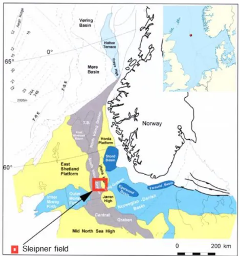
The North Sea Basin is composed of several major Mesozoic graben and highs, dominated by the Viking graben to the north and the Central graben to the south (Gregersen et al., 1997). The Sleipner field is located on the eastern flank of the south Viking Graben, northern North Sea (Figure 4).
Figure 4 - Regional structure map of the northern North Sea and Norwegian continental margin, with the outline of Sleipner field (modified from Kennett, 2008).
From the Permian and throughout the Mesozoic, extensional tectonism dominated the northern North Sea (Gregersen et al., 1997). The north to south trend of the asymmetric Viking graben was developed due to the spread of rifting from arctic areas southwards into the North Sea during the Late Jurassic (Kennett, 2008). This extensional phase was characterized by rapid fault-controlled subsidence, the formation of a series of graben and half-graben basins and clastic syn-rift sedimentation (Fyfe et al., 2003). According to Gregersen et al. (1997), extensional tectonism died out in the Early Cretaceous with the North Sea basin entering a prolonged period of post-rift thermal subsidence and sediment filling supplied by the surrounding
topographic highs. Deposition of thick mud-rich clastic sequences dominated the post-rift sedimentary basin fill corresponding to the Shetland, Rogaland, Hordland and Nordland Groups (Ziegler, 1981).
The Cenozoic era presented six phases of uplift affecting the basin margin and surrounding British and Scandinavian land-shelf areas. These uplifts enhanced erosion of surrounding provenance which resulted in major episodes of siliciclastic sedimentation, mainly during the Palaeocene, Eocene, Oligocene and Miocene, which Galloway et al. (1993) interpreted as onlap defined megasequences. From the Oligocene to Middle Miocene, the northern North Sea basin continued to subside forming a shallow marine sag-basin with deposition of the mud-dominated Hordaland Group (Figure 5) (Head et al., 2004). Three sand-dominated units are also present in the Hordland Group, the Frigg, Grid and Skade formations. Only the Skade Formation is observed in the Hordaland succession in the Sleipner area.
According to Ziegler (1981), the regionally extensive Middle Miocene Unconformity (MMU) marks the top of the Hordaland Group and is particularly prominent on the eastern flank of the basin. It has been interpreted to be a response to uplift of the western Norwegian margin and tilting of the Horda platform, with consequent sub-aerial exposure of the basin margins and a temporary hiatus in sediment supply (Fyfe et al., 2003; Gregersen at al., 1997). A glacial-eustatic sea level fall associated with polar ice cap expansion is interpreted at this time by these authors. Connection between the Norwegian-Greenland Sea and the North Sea became restricted with shallowing and denudation of the uplifted areas resulting in deposition of sand from the rivers draining the Shetland platform to the west and the Norwegian North Sea margin to the east (Fyfe et al., 2003). These sands are the main component of the Utsira Formation in the Viking graben, corresponding to the basal part of the mud-dominated Nordland Group (Gregersen et al. 1997; Fyfe et al., 2003).
Subsidence of the basin during the Pliocene with input from European delta systems from the south-east resulted in large deposition of argillaceous sediments and re-establishment of connection to the Norwegian-Greenland Sea (Fyfe et al., 2003). The Quaternary was dominated by high subsidence and deposition of glaciomarine sediments (Justwan, 2006).
Figure 5- Stratigraphic correlation chart for the Cenozoic Hordaland and Nordland Groups. Sequence stratigraphic schemes: NNS = Northern North Sea; ENS = Eastern North Sea; CNS = Central North Sea (Fyfe et al., 2003).
1.2. Utsira Formation
The Utsira Formation was first defined by Deegan and Scull (1977) and is interpreted as a basin-restricted deposit which constitutes the basal part of the Upper Cenozoic Nordland Group in the northern North Sea (Gregersen et al., 1997; Zweigel et al., 2004), unconformably overlying the Hordaland Group shales (Figure 6). It is mostly composed by mature, well-sorted, fine to medium grained sands which downlap onto underlying mudstones (Fyfe et al., 2003). They are characterized by quartz with subordinate feldspar, rich in bioclastic debris and glauconite which are indicative of marine deposition. The Utsira Sand is clearly identified in well logs with a block low-gamma ray response and presents interbedded clays separating thick sand units. The deposition of the Utsira Formation ranges from late Middle Miocene (c. 11 Ma) to earliest Late Pliocene (c. 3 Ma) as determined based on biostratigraphic data from an exploration well to the south of the Sleipner field (Eidvin et al, 1999).
Regional mapping of the Utsira Formation shows an elongated north-south trending deposit that extends more than 450 km north-south and between 50 and 100 km east-west, which gives an approximate formation area of 26000 km2 (Chadwick et al., 2004a). Its eastern and western limits are defined by stratigraphic onlap onto the Middle Miocene Unconformity and the northern and southern limits are defined by a facies transition into more shaly sediments (Gregersen & Johannessen, 2007). The top of the Utsira Sand surface generally varies smoothly within the depth range of 55-1500m, around 800-900m near Sleipner. Formation thickness maps define two main depocentres (Figure 7), one in the south around Sleipner with thickness reaching 300 m, and one about 200 km to the north, with thickness approaching 200m (Chadwick et al., 2004a). It is interpreted that the deposition of the Utsira Sand was largely sourced from the uplifted East Shetland Platform to the west, with a significant component of Scandinavian-derived material in its northern part (Rundberg and Eidvin, 2002 In Head et al., 2004).
Figure 6– Regional 2D seismic line across the North Sea basin showing the Utsira Sand and the caprock succession. Vertical yellow lines represent well-bore profiles, and the vertical blue lines represent gamma-ray well-log traces (Hermanrud et al., 2010).
The Utsira Sand sediments are defined as basin-restricted marine lowstand deposits but there are a range of interpretations regarding their depositional environment. Some of the work carried out to date have suggested: tidal sand-ridge complexes (Rundberg, 1989); a linked strandplain and sandy shelf shoal deposits (Galloway, 2002); or an amalgamated submarine fan complex (Gregersen et al., 1997). Biostratigraphic data analysed by Eidvin et al. (1999) determined lower rates of sedimentation for the Utsira Sand than of
the overlying shales and considerably lower than the shaly deposits in the Central North Sea which are correlative to the Utsira Sand. Therefore, it has been interpreted by Zweigel et al. (2004) that favourable depositional models should include intensive sediment reworking in a broad channel connecting the Central North Sea and the North Atlantic as well as simultaneous deposition of finer grained or mixed material in the Central North Sea.
The predominant shale sediments of the Hordaland Formation underlain the Utsira Formation. They exhibit severe deformation by soft sediment mobilization and polygonal faulting (Zweigel et al., 2004) which have altered the seismic character of the Hordaland sediments and deformed its top surface (i.e. the Middle Miocene Unconformity - MMU). Hence, mud diapirs and mud volcanoes are present at the base of the Utsira Formation resulting in significant local thickness variations.
The overburden of the Utsira Sand is about 250m thick in the Sleipner area and consists of clay-rich sediments of the Nordland Group (Zweigel et al., 2004). This caprock succession can be divided in three main units (Figure 6): Lower Seal, a shaly basin-restricted unit about 50-100m thick; Middle Seal, prograding sediment wedges of Pliocene age shale-rich in the basin centre but coarsening both upwards and towards the basin margins; Upper Seal, Quaternary sediments mostly glacio-marine clays and glacial tills (Chadwick et al., 2004a).
Figure 7 – Left: Two-way travel time structure map to Top Utsira Sand. Right: Utsira Sand isopach map, showing the two main depocentres. CO2 injection well 15/9-A-16 displayed on both maps (Kirby et al., 2001 In Kennett, 2008).
2. Sleipner CO2 Storage 2.1. Storage Reservoir
In Sleipner, the Utsira Formation is at a depth of 800-1100m below sea level. The CO2 is injected via the deviated well 15/9-A-16 over a 38m perforation interval at about 1012m depth. The high-quality reservoir presents an average porosity of 36%, a permeability range of 1 to 5 Darcy and a net to gross of 98% (Singh et al., 2010).
The Utsira Formation is identified on wireline logs from its low gamma-ray, sonic velocity and neutron density response. The reservoir consists of two units: a lower Utsira Sand unit and an upper Sand Wedge unit which are separated by a 6.5m thick shale unit (Figure 8). The Sand Wedge unit thickens to the east and pinches out to the west. A number of thin spikes of higher gamma-ray, velocity and density log values
are present within the Utsira Sand unit, similar in values to those of the overlying Nordaland shale, corresponding to thin intra-formational shale beds (typically about 1m thick). These thin shale layers constitute important permeability barriers within the reservoir and have proven to have a significant effect on the CO2 plume entrapment and migration.
There is no evidence for faults in the interior of the Utsira Sand (Zweigel et al., 2004). Exceptions are reverse faults at the margins of some mud edifices and more rarely faults from the polygonal faulting pattern of the underlying Hordaland Formation which can be present at the lowermost part of the Utsira Sand, close to its base and below the injection point.
Figure 8 – Gamma ray and sonic wireline log response through the Utsira Formation and the caprock shale. Reservoir characterized by the Sand Wedge, the Thick Shale and the main Utsira Sand units (modified from Kennett, 2008).
Rock samples from the Utsira Sand are almost exclusively ditch cuttings. Limited core data of the Utsira Sand is available from nearby exploration well which consist of weakly consolidated sand that disintegrate when shaken in unfrozen conditions (Zweigel et al., 2004). Thin sections show a homogeneous, fine to medium grained, moderately to well sorted sand with high content of quartz and only minor amounts of cement. Microscopy reveal scarce grain contacts and almost no deformation of the grains confirming the unconsolidated state of the sediment.
The top of the Utsira Sand has been mapped based on wireline logs and 3D seismic surveys corresponding to depths of 750-900m in the injection area. It has a general southward dip on local scale and in detail is gently undulatory with small domes and valleys. The base of the Utsira Sand constitutes an unconformity at depths of 900-1100 m in the Sleipner area. It is structurally more complex with presence of numerous mounds, interpreted as mud edifices (mud diapirs and mud volcanoes) caused by localized mobilization of the underlying Hordaland Shale (Zweigel et al., 2000). Local depressions in the top Utsira level are observed in 3D seismic surveys above mounds at the base Utsira level which can be attributed to preferential compaction of the mud edifices during burial (Zweigel et al., 2004). Therefore, the presence of mud edifices at the base of the Utsira Formation has resulted in significant local thickness variations across the reservoir.
The clay-rich sediments of the Nordland Group Lower Seal are about 250 m thick in the Sleipner area and extend more than 50 km west and 40km east beyond the injection area, corresponding to the primary sealing unit (the caprock). Cutting samples of the caprock from wells in the vicinity of Sleipner indicated grey clay silts or silty clays, generally dominated by illite with minor kaolinite and traces of chlorite and smectite. Caprock core was acquired in 2002 around 20-25 m above the Utsira Sand reservoir and subjected to a detailed testing programme. The core material is typically grey to dark grey silty mudstone, uncemented and plastic, generally homogeneous with weak indications of bedding (Arts et al., 2008). Gas transport testing on core material (Harrington et al., 2008) indicated that the Sleipner caprock has favourable sealing capacities with the ability to hold supercritical CO2 columns in excess of 100 m even up to 400 m depending on the CO2 density, which in turn is sensitive to pressure and temperature at the reservoir top. This is much higher than the buoyancy pressures likely to occur in the Utsira reservoir, where maximum confined column heights are usually less than 10m (Arts et al., 2008).
2.2. Observed CO2 Plume Distribution
An extensive monitoring programme has been carried out over the CO2 injection area. A total of ten 3D seismic surveys and four gravity surveys have been acquired in Sleipner to date to monitor the CO2 behaviour in the storage unit (Furre et al., 2017). A Controlled Source Electromagnetic (CSEM) test line was conducted in 2006 but the resolution was inferior at the time making it challenging to detect the CO2 plume, consequently this study was not repeated. Sea bottom imaging surveys and sampling of sediments and water column have been conducted to investigate possible escape release structures and increased CO2 levels, respectively. None of the monitoring techniques have showed any signs of leakage into the overburden (Arts et al., 2008; Eiken et al., 2011; Furre et al., 2017).
Prior to injection, a baseline 3D seismic survey acquired in 1994 was used to delineate the reservoir geometry. Repeated seismic acquisition to monitor the plume was performed in 1999, 2001, 2002, 2004, 2006, 2008, 2010, 2013 and 2016, respectively. These initial and repeated seismic surveys provide a detailed image of the CO2 plume distribution and dynamics within the storage site.
CO2 is injected into the reservoir in dense (supercritical) state which results in a large contrast in acoustic properties between the brine and the CO2 and favourable conditions for seismic monitoring (Furre et al., 2017). The seismic response from this large acoustic impedance contrast can be observed on the vertical sections of time-lapse seismic surveys as shown in Figure 9. Nine bright reflections were already identified in the first time-lapse repeat survey in 1999, only 3 years after the injection started, indicating that the CO2 ascended more than 200m vertically from the injection point to the caprock. The CO2 plume is evidently layered and asymmetric with a vertical stack distribution indicating that it encountered and breached a series of thin shale barriers (about 1m thick) within the storage site. The thin shale layers acting as baffles to the CO2 migration were identified on well data but, with the exception of the Thick Shale unit that separates the Utsira Sand and Sand Wedge units, it was not possible to correlate them between wells, due to the wide spread of the wellbores (>1km), nor to identify them in the baseline seismic considering its limited vertical resolution (given dominant frequency bandwidth of 20-50 Hz).
A distinct stack of broken reflectors with reduced amplitude strength has become apparent on the time-lapse seismic near the injection point, as can be observed on Figure 9. This vertical feature has been interpreted as a possible main vertical conduct of CO2 in the plume and denoted CO2 chimney (Chadwick et al., 2004b; Bickle et al., 2007). Since it was not possible to identify it on the baseline seismic, its origin, whether it’s a pre-existing feature associated with sand injections from the underlying Hordaland Group
Skade Formation soft-sedimentary deformation (Kennett, 2008; Watsend, 2012) or related to the injection process (Hermanrud et al., 2009), is still debatable. The analysis and incorporation of high permeability chimney features through the intrashales of the Utsira Formation is outside the scope of this thesis.
Figure 9 – Vertical seismic sections across the reservoir representing the 1994 baseline and the CO2 plume growth differences in 2001 and 2008, respectively (courtesy of Equinor).
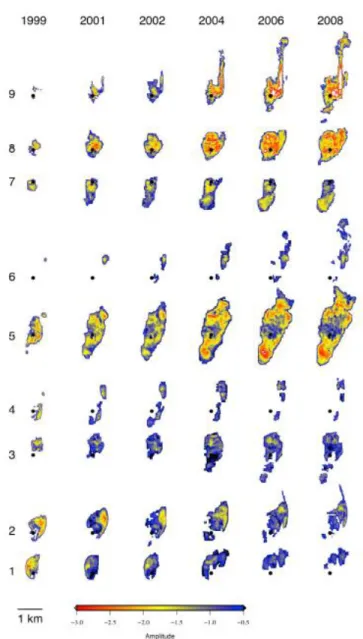
The mapped plume area has reached about 3 km2 by 2008 and time-lapse seismic surveys have shown it has been growing steadily since 1999 (Figure 10) (Eiken et al., 2011). Each of the nine vertically stacked CO2 layers have a pronounced north-south elongation and are estimated about 10-20m thick and a lateral extent of 1-3 km. The nine CO2 accumulations have been interpreted and mapped on the seismic time-lapse datasets, with the lowest observable CO2 layer referred to as layer 1 (L1) and the uppermost CO2 layer as layer 9 (L9). The CO2 layers 1 to 8 are accumulated within the Utsira Sand unit beneath the intraformational thin shales except for L8 which is trapped beneath the Thick Shale unit, and the CO2 L9 is accumulated beneath the caprock within the Sand Wedge unit. The growth and areal distribution of each CO2 layer from 1999 to 2008 can be seen on Figure 11, which is based on amplitude maps through time-lapse seismic data interpreted by Boait et al. (2012). The time-lapse seismic data also indicate that the uppermost CO2 layers tend to follow topographic highs, closely conforming to the mapped topography of the caprock and underlying Thick Shale (Cavanagh et al., 2015).
Figure 10 – CO2 plume in map view based on time-lapse seismic difference reflection amplitude maps, cumulative for all layers. Expansion of the plume in all directions is observed, as well as intensified reflections in the central part of the plume
(Eiken et al., 2011).
The CO2 signatures in the early years of the shallower layers were spatially small and deeper reflectors were easier to interpret. With plume growth throughout the years, shallower layers have become larger, brighter and easier to interpret, impacting the definition of the deeper reflectors. Furre et al. (2017) has attributed the degradation of the deeper signals to a combination of inelastic attenuation, transmission loss of signal through the CO2 layers and CO2 migration and/or dissemination, which reduce the impedance contrast between sandstone and mudstone layers.
Identification of small CO2 saturations in the reservoir as well as potential leakages is very successful in repeated seismic data but quantification of CO2 saturation is difficult. This is because velocities change significantly as the fluid changes from pure brine to a brine with low CO2 saturation, but much less as CO2 saturation increases further (Furre et al., 2017; Boait et al., 2012). Gravity monitoring provide measurements of density changes and consequently of saturation, as density is linearly related to saturation. A baseline for gravity monitoring was acquired in 2002 over the CO2 plume at Sleipner and subsequent surveys were performed in 2005, 2009 and 2013. Based on the gravimetric measurements and the plume geometry from seismic data, a mean in situ CO2 density of 720±55 kg/m3 is estimated, neglecting the effects of dissolution of CO2 into brine (Furre et al., 2017). The amount of supercritical CO2 in the Utsira Formation detected from gravity monitoring is the same as the injected amount of CO2. It is possible to combine the free CO2 mass change and the plume geometry, acquired from gravimetric and seismic data respectively, to make an estimate of CO2 dissolution in water. Considering the temperature estimates for the reservoir, the CO2 brine dissolution rate was estimated between 0% and 2.7% per year, in accordance with measurement uncertainty. This is an important process as it reduces the long-term risk of leakage since the brine with dissolved CO2 is heavier than pure brine and will sink to the bottom of the formation (Eiken et al., 2011).
Figure 11 – CO2 layers lateral expansion as a function of time up to 2008, layers 1 to 9 from base to top of the reservoir. Warmer and colder colour show stronger and weaker amplitudes, respectively; solid black dot shows injection point (Boait et al.,
2012).
3. CO2 Flow Dynamics
3.1. CO2 Storage Flow Dynamics
Carbon dioxide is a gas with density slightly higher than air at surface under atmospheric conditions. At pressure and temperature conditions reached at depths of 800m or deeper, CO2 takes the form of a dense (supercritical) phase in which much larger amounts of mass can be stored per given volume and its density remain much smaller than the resident brine (Andersen, 2017). A storage formation should therefore be at least 800m deep in order to avoid the storage of CO2 in the gas phase which would be very inefficient. This is also the depth at which it is known that geological storage seals are generally effective as gas fields have been contained for millions of years at similar depths.
The injection of CO2 increases the pressure near the well which forces the CO2 to enter the pore spaces initially occupied by in situ formation fluids. The CO2 behaviour in the reservoir is determined by the pressure gradients created by the injection well(s), original hydraulic gradients, and the buoyancy force relative to the original formation fluids (Valberg, 2014). The pressure build-up caused by injection will depend on the rate of injection, permeability and thickness of the reservoir as well as the presence of permeability barriers within it (IPCC, 2005).
In a supercritical state, the CO2 has the density of a fluid but the compressibility of a gas (Arts et al., 2004). This liquid or liquid-like supercritical dense phase of CO2 injected in deep saline formations is immiscible in water (IPCC, 2005). Therefore, it forms a separate mobile dense phase (the CO2 plume) which invades the medium and displaces the formation water that is present in the pore space. Since CO2 is much less viscous than water (by an order of magnitude or more), its mobility is much higher than the brine and this contrast can result in viscous fingering, i.e. CO2 bypassing much of the pore space with only some of the water formation being displaced, depending on the heterogeneity and anisotropy of rock permeability (Flett et al., 2005; IPCC, 2005).
In saline formations, the large difference in density between CO2 and brine (30-50%) creates strong buoyancy forces which drives CO2 upwards until it reaches a baffle or barrier. A lower permeability layer will act as a barrier making the CO2 migrate laterally filling any stratigraphic or structural trap it encounters. Thus, the CO2 plume distribution is strongly affected by formation heterogeneities.
As CO2 migrates through a formation, and their volume fraction reduces below a certain level, they can be retained in the pore space of the formation by capillary forces which may immobilize (store permanently) significant amounts of CO2 and is referred to as residual trapping (Figure 12). Over time, much of the trapped CO2 dissolves into the formation water through a process called solubility trapping. This is a relatively fast process if the brine and CO2 share the same pore space, but once the formation fluid is saturated with CO2, the rate of dissolution slows and is controlled by diffusion and convection rates, which happen as the water saturated with CO2 becomes slightly denser than the original formation water. These processes may take several thousand years to immobilize the CO2 as a dissolved phase in brine. The solubility of CO2 in brine decreases with increasing pressure, decreasing temperature and increasing salinity (IPCC, 2005). The most permanent form of geological storage is mineral trapping, when dissolved CO2 may be converted to stable carbonate minerals, which is a comparatively slow process taking thousands of years or longer. The migration process of CO2 will cease when all the injected CO2 has been permanently immobilized by trapping mechanisms or otherwise leaked back out (Hermanrud et al., 2009). A simple sketch illustrating the dynamics of CO storage can be seen on Figure 13.
Three forces are commonly assumed to determine hydrocarbon flow in the subsurface (Hubbert, 1953 In Hantschel and Kauerauf, 2009). These forces are buoyancy, originated from gravity and density contrast between the hydrocarbon and water; capillary pressure, due to the interfacial tension between the hydrocarbon and water; and friction of the moving fluid, described by viscosity and mobility (Hantschel and Kauerauf, 2009). The reservoir conditions and dynamics between oil and gas production and injection of CO2 for storage are fundamentally different.CO2 storage represents the injection of a non-wetting fluid that displaces the in situ brine which is a drainage process, as opposed to imbibition in hydrocarbon production by aquifer driver or waterflood. This drainage displacement is more typical of regional basin modelling and percolating oil and gas migration (Cavanagh et al., 2015). Therefore, near the CO2 injection well the migration of the non-wetting fluid into the pore space of the rock formation will be due to the pressure gradient under a viscous dominated regime but as the CO2 moves away from the well, gravity and capillary forces will tend to dominate the migration of the buoyant fluid.
Figure 12 – Effectiveness of geological storage in a saline formation increase with time as the physically trapped CO2 plume reacts with to brine becoming more immobile until it gets converted to solid minerals (IPCC, 2005).
Figure 13 – Illustration of the dynamics of CO2 storage. The injected CO2 will migrate upwards due to buoyancy and
eventually fill a structural trap. Some residual trapping of CO2 may be left behind the migrating plume. There will be some
convective mixing of CO2 with brine resulting in dissolved phase trapping of CO2 (Ringrose, 2018).
3.2. Sleipner CO2 Flow Behaviour
CO2 is just at the phase transition between gas and fluid (two-phase flow) at the Sleipner well head. During the 22 years of injection, the well head temperature has been controlled to be stable at 25 degrees Celsius, with pressure consequently also stable at the phase transition around 62-65 bar (Eiken et al., 2011). There are no down-hole pressure gauges as this technology was not readily available when CO2 injection started in Sleipner in 1996 (Furre et al., 2017). However, based on the stable injection rate and 4D seismic imaging showing vertical flow and topography control, it is possible to assume that any pressure build-up is small, implying pressures would only be marginally above hydrostatic. The lack of down-hole data has raised uncertainty in the initial temperature of the Utsira Formation but temperature measurements from a
water producing well at the Volve field, about 10 km north of Sleipner, has narrowed down this uncertainty (Alnes et al., 2011).
The injected CO2 in Sleipner will have temperatures and pressures close to critical point but still in the dense phase in the subsurface (Figure 14). The Sleipner reservoir temperature at the injection point (about 1012m below sea level), based on the nearby well data and on regional knowledge of the temperature gradient, is estimated to be 41 degrees Celsius (Arts et al., 2008). In the North Sea, for geological formations down to about 1500 m below sea level, the pressure is typically hydrostatic.
Figure 14 – CO2 phase behavior for the Sleipner storage reservoir (WH=Well Head, BH= Bottom-hole) and at surface
(vapour around 20 degrees and 1 bar). The injected CO2 is very close to the critical point but still in the dense phase (modified
from Eiken et al., 2011).
The CO2 plume in Sleipner is likely to have ascended due to gravity segregation, given the strong density contrast between CO2 and brine, the high permeability of the Utsira Formation sandstones and the elongated shape of the CO2 plume layers conforming to the caprock and shale topography as observed on time-lapse seismic (Singh et al., 2010; Cavanagh and Haszeldine, 2014; Cavanagh et al., 2015).
III. Dataset
All the data analysed in this master’s thesis is from latest public release from the Sleipner CO2 storage reservoir provided by Equinor. Many research institutes worldwide have worked on Sleipner CO2 monitoring data in the past and a large number of publications exist. Equinor and the Sleipner partners are favourable to the public awareness of the project and its positive effect on the development of CCS in general.
The latest release data package of 4D seismic data covers the CO2 plume in a 3.4 km by 6.1 km area (Figure 15) for the vintages 1994, 1999, 2001, 2002, 2004, 2006, 2008 and 2010. It includes the amount of CO2 injected up to 2010 and coordinates of the injection well perforation (15/9-A-16), as described in more details below.
Figure 15 – Top Utsira TWT and wells in the area. Yellow rectangle shows the coverage of the released seismic data and yellow circle is the location of the injection point (well 15/9-A-16) (courtesy of Equinor).
1. Seismic Data
The 1994 baseline seismic and time-lapse surveys up to 2010 are included in the latest release of the Sleipner CO2 storage data available to the scientific community. The large contrast in acoustic properties between the CO2 and formation brine gives a strong time-lapse response (Figure 16).
The depth converted seismic horizons provided by Equinor for this master’s thesis are Top Sand Wedge, Top Utsira Formation ad Base Utsira Formation (Figure 17). They were interpreted on the 2007 processing of the 1994 baseline seismic data tied to Top Utsira Formation picks in wells 15/9-13 (exploration) and 15/9-A-16 (injector).