Short Term Persistence in Mutual Fund Market Timing
and Stock Selection Abilities
Evangelos Benos and Marek Jochec
∗May 1, 2009
Abstract
Using daily return data from 448 actively managed mutual funds over a recent 9-year period, we look for persistence, over two consecutive quarters, in the ability of funds to select individual stocks and time the market. That is, we decompose overall fund performance into excess returns resulting from stock selection and timing abilities and we separately test for persistence in each ability. We find persistence in the ability to time the market only among well performing funds and in the ability to select stocks only among the very best and worst performers. The existing literature patterns appear only when funds are ranked by their overall performance, which includes stock selection, market timing and fees. With respect to overall performance, there is persistence among most poorly performing and only the top well performing funds. Furthermore, the profitability of a winner-picking strategy depends on the rebalancing frequency and potentially the size of the investment. Small investors cannot profit, whereas large investors can take advantage of the class A share fee structure and realize positive abnormal returns by annually rebalancing their portfolios.
JEL classification: G2
Keywords: mutual fund performance, market timing, stock selection
1
Introduction and Literature Review
Mutual funds are an increasingly popular investment vehicle. As of 2006, they held about 31% of all publicly traded US common stock, up from 4.6% in 1980 and 10.5% in 1990 (French (2007)). Most of these funds are actively managed, with passive funds accounting for only about 13% of all mutual fund holdings in the same year. Furthermore, active fund management is a sizeable industry. Based on the figures reported in French (2007), we calculate the incremental cost of active mutual fund investing to be around $44 billion as
∗The authors are Ph.D students in Economics and Finance respectively at the University of Illinois at
Urbana-Champaign. They can be reached at [email protected] and [email protected]. We would like to thank George Deltas, George Pennacchi, Anne Villamil, Jay Wang and participants of the finance depart-mental seminar at the University of Illinois for helpful comments. All errors are ours.
of 20061. The apparent question is if all this money is well spent and there is a sizeable literature that attempts to answer it.
Active mutual fund management is compensated for seeking to earn positive abnormal returns by attempting to predict returns of individual stocks and/or by attempting to predict the movement of the market or some other systematic risk factor with which stock returns may covary. In the latter case, the fund purchases stocks with a positive factor sensitivity prior to an upward factor movement; otherwise, it either holds cash or purchases stocks with a negative or zero factor sensitivity2.
The early mutual fund literature has empirically established that on average, actively managed mutual funds underperform passive ones3. This perhaps is not a big surprise as there is a well known equilibrium accounting argument to support it: Since passive funds do not trade much, there are small if any net transfers of wealth between active and passive managers. This means that the potential gain of an active manager is the loss of another active manager (the counter-party in the transaction) and thus the average gain among active managers is zero4. Considering that active management is costly and therefore charges higher fees, such funds are bound to yield on average lower returns than passive ones. The difference should be approximately equal to the difference in fees charged by the two types of funds.
Although actively managed funds are on average unprofitable, there is still a possibility that some of them are consistently profitable. In other words, some funds could always generate abnormal gains and others abnormal losses. This is theoretically possible because, as Gruber (1996) points out, mutual funds trade at Net Asset Value. Thus, unlike closed-end funds, ability is not priced. In other words, fund share prices do not adjust to reflect the opinion of the market on a given fund. Another consequence of this is that future performance can be predicted based on past performance. We are quick to point out that this does not necessarily imply that markets are inefficient. The efficiency of the market depends on the possibility to generate abnormal returns; even if a winner-picking strategy is possible, it may not be profitable because of transaction costs and fees.
A number of studies have shown that there is no relative persistence over long time horizons5. This lack of persistence in the long run could potentially be attributed to several factors. One is the diminishing investment opportunities of well performing funds. This scenario is analyzed in Berk and Green (2004)6. The idea is that a manager can exploit a good investment opportunity with only a limited amount of money. Otherwise she will start to have a market impact and the opportunity will be arbitraged away. Another possibility is that management fees rise over time so as to capitalize on a good performance record. Alternatively, once managers have established a good reputation they may be less keen to perform well. Finally, well performing managers may simply wish to exploit their reputation and find a more lucrative job, perhaps in a hedge fund.
1See Appendix 1 for the details of this calculation.
2Mutual funds are restricted to taking long positions in the stock market. Thus, anticipated factor
movements cannot be exploited by short-selling stocks.
3e.g. Jensen (1968)
4See French (2007) for empirical evidence of this.
5e.g. Elton et.al. (1992), Treynor and Mazuy (1966) and Henriksson (1984).
6The Berk and Green (2004) model predicts however that actively managed funds will have zero excess
returns after fees and expenses, which is not supported empirically.
As far as shorter horizons are concerned, there seems to be more evidence for relative persistence in performance. A common conclusion in the literature, however, is that except for the very best fund managers, persistence primarily exists among poor performers7. Market efficiency is easier to support in studies of short-term persistence because of the recurring shareholder fees that a winner-picking strategy requires. In most of the studies of short term persistence, any abnormal returns are eliminated by these fees.
Our paper revisits the issue of short-term persistence in fund managers’ ability. We contribute to the literature by decomposing fund managers’ overall performance into stock picking and market/factor timing abilities. We measure the excess returns resulting from each kind of ability, controlling for excess returns that may be due to other factors, and we investigate if and to what extent these abilities persist over two consecutive quarters. For these persistence tests we follow the same procedure as in Bollen and Busse (henceforth BB) (2004). We first rank funds independently in a given quarter with respect to stock picking and factor timing excess returns and then we see whether the funds preserve their ranking in the subsequent quarter. The quarterly ranking and post-ranking periods force us to use daily return observations so as to efficiently estimate model parameters.
We show that to measure a fund’s ability to time the market, one has to control for the effect of alpha and of potential excess returns that may result from timing or mis-timing the other risk factors of the Carhart (1997) model. When these effects are controlled for, market timing excess returns turn out to follow a different pattern than previously thought: market timing ability is persistent among good performers over two consecutive quarters and the associated excess returns are relatively large. The strong persistence among poor performers as well as the smaller magnitudes of the excess returns that other studies document [e.g. BB (2004)], are due to the effect of alpha and of timing effects from the other risk factors. In the process, we also show that fund managers demonstrate no persistence in timing the other risk factors.
Furthermore, we measure individual stock picking ability by adding back operating ex-penses to the intercept (alpha) of a four-factor Carhart model augmented with convex re-gressors that are intended to control for market/factor timing ability. We find that there is persistence in stock picking ability over two quarters only among the very best and worst fund managers. In terms of overall performance, which is determined by the combination of market timing and stock picking abilities as well as management fees, there is persistence among most poorly performing funds. That is, bad managers are consistently bad. Among well performing funds (i.e. funds with above median performance) only the top decile exhibits persistence.
Finally, we look at the issue of economic significance by testing whether a winner-picking strategy can generate abnormal returns. The marginal investor cannot profitably exploit past information; her returns are eroded by the shareholder fees that are due every time she rebalances her portfolio. This is consistent with the findings of BB (2004). Large investors however can realize profits relative to the Carhart (1997) four-portfolio benchmark by utilizing the breakpoint fee structure of class A shares. Class A shares do not charge shareholder fees for amounts that exceed $1 million and for holding periods that exceed one year. Thus, we repeat our persistence tests for one-year periods and class A shares exclusively and find
that a winner-picking strategy yields an abnormal return of about 1.7% annually. This is in agreement with the results of Hendricks et.al. (1993). Overall, we think that these results lend support to Gruber’s (1996) clientele hypothesis. It seems that although investors in actively managed funds lose money on average, larger and more sophisticated investors have a potential for profit to the detriment of the small and unsophisticated ones. Furthermore, the existence of a profitable strategy is inconsistent with semi-strong market efficiency and this may partly explain why so much money is consistently invested with actively managed funds.
In the rest of the paper we describe our data set (Section 2), we explain our methodology (Section 3), we present the results (Section 4) and conclude (Section 5).
2
Data and Summary Statistics
Our main data set consists of daily returns of 448 actively managed mutual funds. The returns are net of fund operating expenses. Thus, they include management and distribution fees, but not sales loads8. We obtain these observations from the CRSP mutual fund daily database. We also use fund names and investment objectives which we obtain from the CRSP mutual fund annual database. The funds in both databases are identified by a “CRSP-FUNDNO”9. Our time range is a 9-year period starting on January 1st, 1999 and ending on December 31, 2007 10.
To obtain this data, we apply several filters on our initial set of observations. Since we are interested in fund managers’ stock selection and timing abilities we restrict our attention to domestic equity funds. The Lipper fund classes included are the following: EIEI (Equity Income Funds), G (Growth Funds), LCCE (Large-Cap Core Funds), LCGE (Large-Cap Growth Funds), LCVE (Large-Cap Value Funds), MCCE (Mid-Cap Core Funds), MCGE (Mid-Cap Growth Funds), MCVE (Mid-Cap Value Funds), MLCE (Multi-Cap Core Funds), MLGE (Multi-Cap Growth Funds), MLVE (Multi-Cap Value Funds), SCCE (Small-Cap Core Funds), SCGE (Small-Cap Growth Funds) and SCVE (Small-Cap Value Funds). The Lipper objective codes however still include funds that are not actively managed and/or are not invested in domestic equity and/or are restricted in specific industries11. To eliminate these funds, we search for keywords in the fund names that would indicate an undesired category (such as “government”,“real estate”, “international”, etc.) and drop from the sample all funds whose name contains such a keyword. In addition, we require that the funds have more than a year (252 trading days) of daily returns, more than $20 million of average annual Total Net Assets (TNA) during the fund’s life and a turnover ratio above 10%. We also require that they have non-missing returns for at least 95% of trading days for the period when the fund is listed in the daily database. Finally, we eliminate all younger share classes of those funds that have multiple share classes12.
8For a detailed description of the mutual fund fee structure see “http://www.sec.gov/answers/mffees.htm”. 9Starting from May 2008, CRSP dropped the ICDI identifier and introduced the “CRSP-FUNDNO”. 10Daily returns in the CRSP mutual fund daily database start from September 1998; however, Lipper fund
investment objectives are reported from 1/1/1999. To determine fund objectives in 1998 we could have used Strategic Insight’s investment codes, but to keep things simple we excluded the four months of 1998.
11Examples include real estate funds, money market funds, government securities funds etc.
We end up with a total of 10,232 fund-quarters and 644,616 daily observations. The average life of a fund in our dataset is 6.5 years (23 quarters). Of the total 448 funds, 162 of them survive for the whole time period of our study, 139 funds were present in the beginning but later dropped, 124 funds entered at some later point and made it to the end of the sample time and the remaining 23 funds entered and exited our sample in between the beginning and end of the time period we examine. Table 1 shows annual statistics for the turnover ratio, the expense ratio, management fees and loads. It also reports the number of funds in our dataset every year and their average Total Net Assets (TNA).
3
Methodology
Overall Manager Performance
We measure a manager’s overall performance by Carhart’s alpha. This is the estimated intercept from the regression:
Rpt− Rf t = αp+ β1p(Rmt− Rf t) + β2pSMBt+ β3pHMLt+ β4pMOMt+ upt (1) where Rpt is the manager’s realized return in period t, Rf t is the risk-free rate and Rmtis the market return over the same period. SMBtand HMLtare the values of the the Fama-French (1993) size and book-to-market factors and MOMtis the period t value of the Carhart (1997) momentum factor.
Being the intercept of model (1), Carhart’s alpha measures managers’ overall performance because it picks up any returns in excess to those predicted by the systematic risk factors. These excess returns are determined by the ability of managers to select individual stocks, by their ability to time the market or some other risk factor, and by management fees.
The risk factors used in (1) have been shown to have explanatory power in the cross-section of stock returns and are included in the calculation of the benchmark return so as not to reward managers for taking advantage of well-known systematic anomalies in the stock market. Since most of the funds in our sample have specific investment objectives which they meet by holding specific asset classes, using the four factor model is essential in accurately measuring managers’ ability.
Market/Factor Timing Ability
A manager who wishes to time a systematic risk factor will purchase stocks that have a sig-nificant and positive sensitivity to that factor in anticipation of an upward factor movement. In the case of an anticipated downward factor movement, the manager will either switch to stocks with a small (or negative) sensitivity to the factor, or will simply hold cash. This will cause the manager’s conditional realized returns to be a convex function of the risk factors. Thus, as is common in the literature, we measure a manager’s ability to time some risk factor by a term that captures this convexity of the realized returns. For each mutual fund p and for
strip everything after the semicolon, sort by the remaining portion of fund name and inception date, and keep the earliest record.
a multi-factor model of stock returns, the following specification is estimated over N trading days: Rpt− Rf t = αp0 + 4 X i=1 βipfit+ 4 X i=1 γipg(fit) + ²pt, t = 1, 2, ..., N (2) where fitis the value of factor i at time t and i = 1, 2, 3, 4 denotes each of the four risk factors in the order they appear in equation (1). The function g(.) is in our case either g(fit) = fit2 or g(fit) = fitI[fit≥0]. We should mention that it is important to control for timing ability
in all risk factors even when one is only interested in measuring the ability to time a single factor. Otherwise, it is impossible to tell apriori if the estimated coefficient captures the timing ability of the particular factor. Unless g(fit) ⊥ g(fjt) ∀j 6= i, a model that includes a single timing factor will yield inconsistent estimates, since the estimated coefficient will also capture any timing effects from the other factors.
The average daily excess return that results from timing factor i over these N trading days, is given by:
ri,p = ˆγip 1 N N X t=1 g(fit) (3)
where ˆγip is estimated from (2). The average daily excess return that results from timing all factors is: rp = 1 N 4 X i=1 N X t=1 ˆ γipg(fit) (4)
Finally, we also report the daily total excess return that includes individual stock picking and factor timing excess returns as well as management fees:
rc,p = ˆα0p+ 1 N 4 X i=1 N X t=1 ˆ γipg(fit) (5) ˆ α0
p is also estimated from (2) and can be interpreted as the cost of implementing a timing strategy. The total excess return rc,p should generally be similar in magnitude to the four-factor alpha from model (1) because both measures capture overall manager ability. If there are any differences between the two, these should be caused by mis-specification of the timing effects in model (2).
Individual Stock Picking Ability
In addition to market timing, a mutual fund manager may possess the ability to select individual stocks that perform well regardless of market/factor movements. We attempt to measure this ability as well.
Since fund returns are net of management fees and other operating expenses and since factor timing effects are controlled for in model (2), the intercept ˆα0
p captures a manager’s individual stock picking ability net of management fees and other expenses. Thus, to obtain a measure of stock picking ability we need to add operating expenses back to ˆα0
p. The reported fund operating expenses are however average expenses across fund share classes which means that we cannot simply use the oldest share class for each fund. Instead, we
need to first calculate for each fund the daily TNA-weighted returns over all share classes. We then estimate model (2) for each fund-quarter anew and add the daily expense ratio13 to the estimated intercept. The daily expense ratio is just the annual expense ratio divided by the number of trading days. Thus, the daily excess return due to stock picking ability for fund p over a given quarter is:
rs,p = ˆα0p+ ExpRatiop/252 (6)
where ˆα0
p has been estimated using the TNA-weighted returns of all fund share classes.
Testing for Persistence in Managers’ Ability
The issue of persistence in managers’ ability to select stocks and time risk factors has two dimensions. First, one can ask if some managers who did particularly well or poorly over the past quarter continue to do so in the next. That is, one can examine if there is persistence in a particular performance subgroup of fund managers. The second question is if managers exhibit persistence in general. That is, no matter what the performance over the previous quarter was, it remains unchanged in the next. In this paper we address both of these issues. To test for persistence in ability in different manager performance subgroups, we follow the procedure in BB (2004). For each fund and over consecutive quarterly periods (63 trading days), we use daily fund and factor returns to estimate Carhart’s alpha, the excess returns in (3) and (4) that result from factor timing, the total excess return (5) and the stock picking excess returns in (6). We then rank the funds according to their alphas and excess returns and form decile portfolios based on these rankings. Since we work with both functional forms of g(.), we do a total of 15 independent rankings for each quarter. We then calculate average decile portfolio alphas and excess returns (these are just the simple averages of the alphas and excess returns of the funds in the particular decile portfolio) and report the time-series average alphas and timing excess returns over all quarters, for each decile portfolio. The last step is to re-estimate the alphas and timing/stock picking excess returns again, for each decile portfolio, in the subsequent quarter. If well/poorly performing deciles preserve their ranking and generate significant returns in the subsequent post-ranking quarter, then we have evidence of short-term persistence in ability for the particular subgroup.
Bootstrap Tests
There is a potential problem with the post-ranking tests of excess return significance. If there is persistence in ability for one or more subgroups of managers, then for a given fund in such a subgroup, the alphas and excess returns estimated over a quarter will be correlated to the alphas and excess returns estimated over other quarters as well. Thus, the independence assumption, required for a parametric test of whether the mean of alphas/excess returns in a decile portfolio equals zero, may be violated.
To address this issue, we calculate bootstrap p-values as follows: We first re-sample (with replacement) the observations in each fund-quarter of a decile portfolio and re-estimate the
13The expense ratio is the ratio of the fund’s annual operating expenses to the average annual TNA. It
fund-quarter alpha and excess returns. Doing this for all fund-quarters enables us to calculate a single bootstrap mean alpha/excess return. This procedure is repeated 1000 times and gives rise to the empirical distribution of the alpha/excess return means. We finally assess the significance of the original mean alpha and excess return of a particular decile portfolio based on this empirical distribution.
Average Persistence
To test for persistence on average, we regress, for each quarter and across funds, a given performance measure on its value in the previous quarter:
Perfp,t = at+ btPerfp,t−1+ ²p,t p = 1, 2, ... (7)
where Perfp,t is any of the performance measures (alphas, stock picking/factor timing excess returns) that we have considered so far. With this, we obtain a time-series of estimated coefficients {ˆat, ˆbt}36t=1, one for each quarter. Then, we test if the time-series averages of the coefficients (¯ˆa,¯ˆb) are statistically different from zero. A significantly positive ¯ˆb would indicate that fund managers on average exhibit persistence with respect to a particular performance measure.
Survivorship Bias Considerations
In principle our data does not suffer from survivorship bias because we include the funds that ultimately disappear. However, we do restrict our sample to include quarters for which all 63 daily observations are available. This means that if a fund survives for 5.5 quarters, the observations of only the first five quarters will be retained and those of the last half quarter will be discarded. A fund may disappear either because it goes out of business or because it merges with another fund. In the first case, the elimination of the last days of a fund’s life does not necessarily bias our results in any direction. This is because we are concerned with excess returns whereas the survival (or not) of a fund is more likely related to its raw returns. This may not be true however in the case of a merger. Ding (2008) finds that the funds that get absorbed tend to under-perform (i.e. have negative alphas) prior to being acquired. To the extent that there is persistence in performance in the short run, this likely biases the results against the persistence hypothesis. This is because funds that would have otherwise under-performed in (say) two consecutive quarters and thus would have exhibited persistence in negative performance, in our case merge in the second quarter and thus exit our sample.
4
Results
Persistence Among Mutual Fund Subgroups
We start by examining if there is short-term persistence in ability, among performance sub-groups of mutual fund managers. Table 2 shows average daily abnormal returns over all ranking quarters, for the 10 decile portfolios. We report Carhart’s alpha as a measure of
overall performance and factor timing excess returns as a measure of factor timing ability. For the latter, we report excess returns for both the quadratic and piecewise linear functional forms of g(.). We also report total excess returns (defined in (5)). To the extent that the quadratic and piecewise linear factors of model (2) accurately capture market/factor timing effects, total excess returns should be similar in magnitude the four-factor alpha.
The top decile portfolio exhibits a daily overall abnormal return of 0.0878% and the bottom decile portfolio a return of -0.0915%. These numbers correspond to 5.7% and -5.6% respectively over the quarter (24.8% and -20.6% over the year). Notice that the average alpha across decile portfolios is negative. This is consistent with much of the earlier mutual fund literature and is the main reason why the profession has come to conclude that on average mutual fund managers do not create value.
Regarding total excess returns, the variability between the top and bottom decile port-folios is also large. Contrary to BB (2004), the two specifications give substantially different results with the piecewise linear one generating much more contrast than the quadratic spec-ification. However, we think that the quadratic specification is more accurate. The reason is that the piecewise linear specification assumes that a market timer can tell when the market (or potentially some other risk factor) will register positive or negative returns as it places the “kink” of the realized returns at zero. It is however more plausible to assume that tim-ing ability is imperfect, in that managers can only predict if the market will register higher or lower returns relative to a historical average. In this case, the “kink” in the manager’s realized returns will not be located at the origin, although the general pattern of realized returns will still be quadratic. This means that a piecewise linear model will be misspecified, whereas a quadratic model, which makes no assumptions about the location of the kink, will not. This intuition is confirmed by the fact that the quadratic specification total excess returns are much closer to Carhart’s alpha than are the total excess returns of the piecewise linear specification.
For both specifications, the average market timing excess return is positive and larger than the other risk factor excess returns. This suggests that managers do attempt to time the market at least in a quarterly time frame and on average they are successful. In doing so, they seem to mis-time SMB and HML and thus the combined factor timing excess return (rp) is smaller in magnitude. However, when one also takes into account stock picking and management fees, the total excess return is on average negative for both specifications. Overall, Table 2 provides a benchmark for assessing the magnitude of excess returns in the post-ranking quarters.
Table 3 presents the results of the tests for persistence in overall performance and tim-ing abilities, among ranktim-ing quarter performance subgroups. It shows the average daily four-factor alphas in the post-ranking quarters as well as the excess returns resulting from market/factor timing. Since the funds that populate each decile were selected over the previ-ous quarter, any significant abnormal returns that preserve the ranking in these post-ranking quarters are indicative of persistence in performance for the particular fund subgroup. Sta-tistical significance is determined by bootstrap standard errors.
The post-ranking alphas are significant and with the same sign as the ranking alphas only for the single best performing and the bottom half deciles. This suggests that good overall performance persists only among the very best stock pickers while persistence in poor overall performance is much more widespread. Regarding magnitudes, the top and bottom
decile excess returns amount to 0.70% and -0.82% over the quarter respectively. The sign reversals for deciles 3 to 5 suggest that some of the positive alphas in the ranking quarter were probably spurious. In general, the post-ranking alphas are similar in magnitude to those of other studies (e.g. BB (2004)) and they are also in agreement with earlier work showing poor performance to be more persistent (e.g. Carhart (1997)).
Turning to the timing ability excess returns, a look at Table 3 reveals that there is persistence in market timing primarily among well performing fund managers: the top deciles exhibit the highest positive market timing excess returns, while the excess returns of the bottom half deciles are smaller. The excess returns of the top deciles are 0.86% and 1.79% on a quarterly basis for the quadratic and the piecewise linear specification respectively, although, as we explained earlier, we have more faith in the results of the quadratic specification. These market timing excess returns are much larger than the ones reported by BB (2004). This is apparently because we control for the effect of alpha which is on average negative14. On the contrary, the excess returns resulting from timing the SMB, HML and momentum factors are for both specifications either of the opposite sign relative to the ranking quarters, or statistically insignificant15.
When the combined effect of all the risk factors is considered, there is no persistence in the total factor timing excess return rp. We conjecture that when managers engage in market timing, they load their portfolios with stocks that are poorly timed with respect to SMB, HML and momentum. Thus, so far the evidence suggests that some mutual fund managers possess market timing ability, which persists for at least two quarters, but they have no ability or intent to time the other systematic risk factors. Furthermore, although good market timers exhibit persistence over two consecutive quarters, their poor stock selection ability and/or high management fees almost completely eliminate their market timing excess returns: although the average market timing excess return is positive, the average overall excess return (Carhart’s alpha) is negative.
As we mentioned earlier, our market timing excess returns are larger than the ones re-ported by BB (2004). This is because they report excess returns that result from both stock picking, market timing and operating expenses. In particular, BB (2004) estimate:
Rpt− Rf t = αc,p+ 4 X
i=1
βpifit+ γ1,pg(f1,t) + ²pt, t = 1, 2, ..., N (8) and then report:
rBB1,p = ˆαc,p+ ˆγ1,p 1 N N X t=1 g(f1t) (9)
where f1t = Rmt − Rf t and both ˆαc,p and ˆγ1,p are estimated from (8). However, there are two potential problems with this approach. First, the excess return rBB
1,p can be heavily influenced by ˆαc,p. This means that we do not know ex-ante if the market timing excess return is itself significant and persistent, or if the significance and persistence is driven by alpha.
14Later on, we show that it is important to remove the effect of alpha if one is to accurately estimate factor
timing excess returns.
15For SMB in particular, there seems to be a significant performance reversal of the best performing funds
Second, the market premium quadratic term may capture potential quadratic variations of the other factors which would render ˆγ1,p biased. The first problem has potentially more serious consequences. To illustrate this, we estimate (8) for g(fi,t) = fi,t2, each time using a different risk factor for the quadratic term16. We then calculate rBB
i,p , rank funds by this metric, and create decile portfolios in the ranking and post-ranking quarters in the exact same fashion as before. The results are in Table 4. Panel A lists the average (across funds and quarters) excess returns of the decile portfolios in the ranking quarter and Panel B lists the excess returns over the post-ranking quarters. The most striking feature of Table 4 is that the excess returns are similar both in magnitude and persistence patterns, no matter which risk factor is used for the quadratic term in specification (8). Thus, if one replicated the BB (2004) procedure using some risk factor other than the market premium, one would have concluded that there is persistence among the poorly performing timers of the particular risk factor. To facilitate comparison, the rightmost column shows the results of the BB (2004) paper.
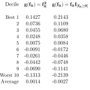
We next test if there is persistence in the ability of mutual fund managers to select individual stocks. As a measure of this ability we use rs,p (defined in (6)), the estimated intercept of model (2) with operating expenses added back. Table 5 shows the average daily values of rs,pfor the ten decile portfolios, for both specifications, during the ranking and post-ranking quarters. Although the two specifications yield results that differ in magnitude, there seems to be persistence among the best and worst stock pickers. For the worst performers in particular (funds in decile 10) , both models yield similar results in terms of magnitude and statistical significance.
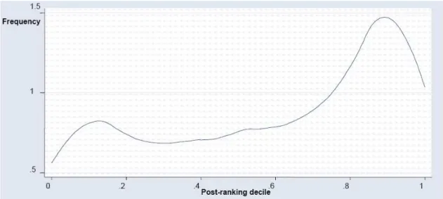
To illustrate how the funds in the top and bottom ranking quarter percentiles behave in the post-ranking period, we plot in Figures 1-6 the distributions of post-ranking quarter rankings for three performance measures: Carhart’s alpha, the market timing excess return
r1,p and the stock picking excess return rs,p. The first thing to observe is that there are funds that migrate even to the complete opposite performance percentile in the post-ranking quarter. However, for all performance measures, the mode and most of the mass of the distribution lies on the ranking quarter percentile suggesting that there is short-term per-sistence in performance. It is also interesting to notice that for most performance measures a significant probability mass lies above the extreme opposite performance percentile, thus rendering these conditional distributions bimodal.
Finally, in Table 6, we show the relationship between measures of overall performance, stock picking and market timing abilities on one hand, and such fund attributes as turnover and management fees on the other. We rank funds every quarter by each of the performance measures and then report the average (across quarters) management fee and turnover ratio of each decile. Management fees and turnover ratios are correlated and vary significantly across deciles. The best and worst performers are the most active traders. It seems that successful stock picking and market timing requires a fair amount of active trading but the opposite is not true: active traders are not necessarily good stock pickers or market timers. Management fees seem not to reward performance but trading. As a consequence, the best and worst performers charge the highest fees. Although this relationship was known to exist
16The results for g(f
for measures of overall performance17 it seems that it also exists for the measures of market timing and stock picking abilities as well.
Persistence Among Mutual Funds on Average
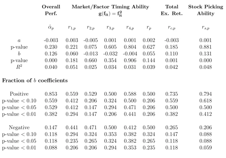
In this short section we examine if there is persistence on average in mutual fund managers’ overall performance and their stock picking and market timing abilities. In Table 7 we show the results of regression (7) for the quadratic functional form of g(fit)18. The coefficient of interest is b with positive and significant values implying that there is persistence on average with respect to a particular performance measure.
The results suggest that there is strong aggregate persistence in overall performance as measured by alpha. The point estimate of b is positive at 0.126 and statistically significant at 1%. The fact that b < 1 implies that the post-ranking quarter excess return is lower than the ranking quarter excess return, which is also evident from Table 3. A similar persistence argument can be made for the total excess return rc,p. It seems however that this persistence is primarily driven by managers’ stock selection ability. The coefficient b for rs,p is positive and highly significant, whereas that of rp is not. That is, there is no persistence in the individual and total factor timing excess returns as suggested by the high p-values of b. Apparently, for these returns there are on average too many sign reversals from the ranking quarters to the post-ranking ones so that no average persistence can be established. For rc,p,
rs,p and for Carhart’s alpha, the fraction of significantly positive b coefficients is also much larger than that of the significantly negative ones.
Potential Biases in the Estimation of Timing Coefficients
There are at least two factors that could potentially bias the timing coefficient estimates ˆγi,p in model (2). Here we discuss them and assess their implications.
One potential issue is the cash flow bias described in Warther (1995). The idea is that when the market does well, funds attract more capital and - to the extent that they have limited investment opportunities - their cash holdings increase. The increased cash holdings lower their sensitivity to the market, in these good times, and thus their realized returns. As a result, the estimated timing coefficients will be biased downward and will understate the manager’s true timing ability. Although we cannot correct this bias, it does not negate our results because it is in the opposite direction of what we want to show. Had it not exist, our timing ability coefficients would have been larger in magnitude and probably more significant.
A more serious concern is that the estimated timing coefficients of model (2) may be spurious if the funds hold portfolios that are more option-like than the market proxy portfolio. This point is made in Jagannathan and Korajczyk (1986). To illustrate, consider a fund manager who has no timing ability. If this manager does have the ability to pick stocks with a call-option-like sensitivity to the market, then estimation of model (2) will still yield positive and significant coefficients for the quadratic terms. This is an upward bias and we have to account for it.
17e.g. Grinblatt and Titman (1994)
For this, we repeat our tests using synthetic funds in the spirit of BB (2001). The goal is to construct funds that imitate the actual ones in terms of style but which by construction exhibit no timing abilities. If the timing excess returns of the synthetic funds are significantly smaller than the those of the actual ones, then we can conclude that the timing excess returns of the actual funds are not the result of the above bias. Appendix 2 details the construction of the synthetic funds.
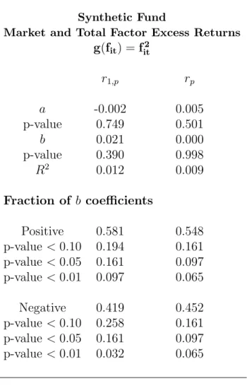
The results of the synthetic fund tests appear in Tables 8 and 9. In Table 8 we show the ranking and post-ranking quarter estimates of r1,p and rp, the market and total timing excess returns19. Clearly, the hypothesis of persistence over two quarters is rejected as no decile portfolio exhibits statistically significant excess returns. Furthermore, the ranking of the decile portfolios is not preserved. Table 9 shows the results of regression (7) for the synthetic funds. Again, the coefficient of interest, b, is insignificant indicating that there is no persistence whatsoever. This suggests that our earlier findings are not spurious and cannot be attributed to mismeasurement of timing ability.
Economic Significance
Since the top performing mutual funds exhibit persistence over two consecutive quarters, it is valid to ask if an investor could exploit this and realize economically significant excess returns. The strategy an investor would have to follow would be a “winner-picking” one, whereby every quarter the investor would rank funds by performance and purchase the top performing ones. Thus, the mutual fund portfolio would have to be rebalanced every quarter. This means that any stock picking and/or market timing excess returns could be eroded by shareholder fees that are paid every time a fund share is purchased20.
The daily value of Carhart’s alpha for the top performance decile portfolios in the post-ranking quarters is 0.0111%, or 0.70% per quarter. We need to compare this number to the cost of executing a winner-picking strategy. Although our data consists of funds that belong to different share classes with varying loads, a minimum load of 1% is often charged by all share classes for holding fund shares less than a year, regardless of the amount being invested21. However, the quarterly cost of executing a winner-picking strategy also depends on the fraction of funds in the top decile portfolio that need to be rebalanced from quarter to quarter. We estimate the average of this fraction over all quarters in our data to be 81%. Thus, the quarterly cost of executing a winner-picking strategy is 0.81% and exceeds the quarterly abnormal return of 0.70%. The conclusion is that it is not possible to execute a profitable winner-picking strategy that involves quarterly rebalancing.
Large investors could potentially make a profit by executing a winner picking strategy with annual rebalancing, using exclusively class A fund shares. Class A shares charge front-end fees which are proportional to the amount invested; for amounts that exceed one million dollars, investors are usually excused from any fees provided they hold the fund shares for at
19Here we report results from the quadratic specification. The results for the piecewise linear specification
as well as the excess returns of the other risk factors are qualitatively similar and we omit them.
20Fund returns are already net of operating expenses.
21There are of course funds that are truly “no load” and charge no shareholder fees regardless of the holding
period. It is not clear however if a winner-picking strategy could be executed using these funds as there may not be many of them. Here we take a more conservative approach and generally assume a 1% load.
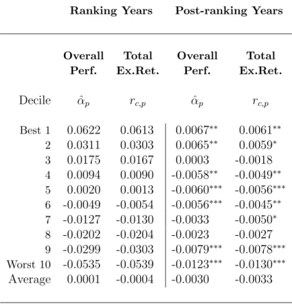
least a year. To see whether such a strategy would be profitable, we repeat our persistence tests using this time annual ranking and post-ranking periods. In Table 10 we report average daily Carhart’s alphas and total excess returns in the ranking and post-ranking years. The top decile post-ranking alpha is 0.0067% on a daily basis or 1.7% annually. This time the investor is not faced with any loads and thus she reaps the entire excess return. Thus, there seems to exist a winner-picking strategy that is profitable. It requires an amount that exceeds $1 million, annual rebalancing and investment in class A fund shares.
The fact that a winner-picking strategy is profitable is inconsistent with semi-strong market efficiency, since information on past returns can be exploited to consistently yield positive abnormal returns.
5
Summary and Conclusion
In this paper we use a data set of 448 actively managed US equity mutual funds to re-examine short term persistence in their performance. In particular, we decompose overall manager performance into stock picking and market/factor timing abilities, we measure each component and we test for persistence over two quarters.
By controlling for the effect of alpha and for mistiming of the other risk factors, we show that managers’ ability to time the market persists strongly among well performing market timers. Furthermore, there is no sign of persistence in timing the other risk factors of the Carhart (1997) model. We also show that unless one controls for the effect of alpha and of the other risk factors in calculating factor timing excess returns, the results are biased and as a result one can show timing persistence not only for the market but for every factor indi-vidually. We measure the ability of managers to select individual stocks by adding operating expenses back to the intercept (alpha) of a model that already controls for timing ability. We find that only the very best and worst managers exhibit persistence in the ability to select stocks.
In terms of overall performance, our analysis confirms earlier findings in the literature. Funds exhibit persistence in their overall performance and this is much more pronounced for poorly performing funds. Among well performing funds, only the top performers exhibit such persistence. The gains from a winner-picking strategy that a typical small investor would expect to realize are eliminated by sales charges. This is largely because these charges are paid at least four times a year since a winner-picking strategy requires quarterly rebalancing. On the other hand, a large investor who chases winners by utilizing the breakpoint fee structure of class A shares and rebalances the portfolio every year, realizes a 1.7% excess return. Thus, our results are inconsistent with semi-strong market efficiency. The fact that large investors can profit from this inefficiency and small ones cannot, lends support to a clientele hypothesis (as in Gruber (1996)) whereby unsophisticated investors invest in actively managed funds regardless of performance and sophisticated investors take advantage of this.
Appendix 1
Here we calculate the incremental cost of active mutual fund management in 2006. All the numbers used are from French (2007). The incremental cost of active management in mutual funds equals the actual amount spent on active management less the amount that would be spent had all the money invested in active funds been invested in passive funds instead. In 2006, the combined market capitalization of US stocks listed on NYSE, Nasdaq and AMEX was about $15,450 billion. Of this, 30.5% (or $4,712.25 billion) was held by all mutual funds and of this, 87.4% (or $4,119 billion) was held by actively managed ones.
The cost of fund management as a percentage of asset value is the sum of a fund’s expense ratio and its annuitized load. French does not explicitly report the cost of active mutual fund management but he does report the average cost of all mutual funds (active and passive) in 2006 which is 100 bps, as well as that of passive funds only (6.5 bps). From these two numbers and the respective equity holdings one can back out the cost of active fund management by solving:
87.4% × ActMgmCost + 12.6% × 6.5bps = 100bps
The cost of active management is thus 113 bps or $46.5 billion (1.13% × $4, 119billion). If the $4,119 billion were invested in passive funds instead, the management cost would have been $2.7 billion (0.065% × $4, 119billion). The difference between the cost of active and passive management (incremental cost) in 2006 is thus about $43.8 billion.
Appendix 2
We pair each mutual fund with a synthetic one that is intended to mimic its style but exhibits by construction no timing ability. The first step in this process is to calculate daily risk-factor values. We start from the CRSP universe and apply a number of filters. We exclude stocks with fewer than 12 monthly returns and/or 252 daily returns, missing prices and numbers of shares outstanding, prices smaller or equal to $1 on any given day, missing or negative book values, and share codes other than 10 or 11 (to exclude foreign stocks, ADRs, shares of beneficial interest, depository partnership units and receipts, trusts, closed-end funds, and REITs). The risk factors are the daily returns of six B/M-size and two momentum portfolios. The six B/M-size portfolios are formed by the intersection of two size and three B/M portfolios constructed by independent sorts. The two momentum portfolios consist of the top and bottom 30% of all stocks sorted by last year’s raw returns.
The next step is to determine the sensitivity of a fund to these factors. For that, we express the fund returns as:
Rp,t= 8 X
i=1
bp,iri,t+ ²p,t (10) where ri,t is the day t value of risk factor i. We estimate the bp,is by minimizing the variance of ²p,tsubject to a non-negativity constraint for the estimated coefficients. For this estimation we use all the daily returns available over the fund’s life.
Once the sensitivities of a fund to the risk factors have been estimated, we construct the mimicking synthetic fund by randomly selecting 100 stocks from the eight factor portfolios in proportions determined by the estimated sensitivities. Thus, the proportion of stocks selected
from factor portfolio i is ˆbp,i/ P8
i=1ˆbp,i. The synthetic fund is initially an equally weighted portfolio of these 100 stocks, but its returns evolve according to a buy-and-hold strategy. To account for the possibility that some of the selected stocks change characteristics over time and are thus no longer representative of the initial factor portfolio, we replace these stocks at random intervals. The average time each of the stocks spends in the synthetic fund is about one year.
References
Berk Jonathan and Richard Green, 2004, “Mutual Fund Flows and Performance in Rational Markets”, Journal of Political Economy, Vol. 112, No. 6, 1269-1295.
Bollen Nicolas and Jeffrey Busse, 2001, “On the Timing Ability of Mutual Fund Managers”,
Journal of Finance, 56, 1075-1094.
Bollen Nicolas and Jeffrey Busse, 2004 “Short-Term Persistence in Mutual Fund Perfor-mance”, The Review of Financial Studies, 18, 569-597.
Carhart Mark, 1997, “On Persistence in Mutual Fund Performance”, Journal of Finance, 52, 57-82.
Ding William, 2008, “Mutual Fund Mergers: A Long Term Analysis”, working paper
Elton Edwin, Gruber Martin, Das Sanjiv and Matthew Hlavka, 1993, “Efficiency with Costly Information: A Reinterpretation of the Evidence for Managed Portfolios”, Review of
Finan-cial Studies, 6, 1-22.
Fama Eugene and Kenneth French, 1993, “Common Risk Factors in the Returns on Stocks and Bonds”, Journal of Financial Economics, 33, 3-56.
French Kenneth, 2007, “The Cost of Active Investing”, working paper.
Grinblatt Mark and Sheridan Titman, 1994, “A Study of Monthly Mutual Fund Returns and Performance Evaluation Techniques”, The Journal of Financial and Quantitative
Anal-ysis, No. 3, 419-444.
Gruber Martin, 1996, “Another puzzle: The Growth in Actively Managed Mutual Funds”,
Journal of Finance, 51, 783-810.
Hendricks Darryll, Jayendu Patel and Richard Zeckhauser, 1993, “Hot Hands in Mutual Funds: Short-Run Persistence of Mutual Fund Performance, 1974-1988”, Journal of Finance, 93-130.
Henriksson Roy, 1984, “Market Timing and Mutual Fund Performance: An Empirical Inves-tigation”, Journal of Business, Vol. 57, No. 1, pt. 1, 73-97.
Jagannathan Ravi and Robert Korajczyk, 1986, “Assessing the Market Timing Performance of Managed Portfolios”, Journal of Business, 59, 217-235.
Jensen Michael, 1968, “The Performance of Mutual Funds in the Period 1945-1964”, Journal
Securities and Exchange Commission (SEC) website: www.sec.gov
Treynor Jack and Kay Mazuy, 1966, “Can Mutual Funds Outguess the Market?”, Harvard
Business Review, 44, 131-136.
Warther Vincent, 1995, “Aggregate Mutual Fund Flows and Security Returns”, Journal
Table 1: Cross-fund averages of various fund characteristics for each of the years of our sample. The Turnover Ratios, the Expense Ratios, the Management Fees and the Loads are expressed as % of Total Net Assets. Total Net Assets (TNA) are in millions of dollars.
Year No. of Funds Turnover Expense Management Front Rear TNA
Ratio Ratio Fee Load Load ($ million)
1999 328 92 1.2 0.68 3.8 2.3 898 2000 308 101 1.2 0.64 4.2 2.3 849 2001 322 100 1.2 0.74 4.7 2.3 680 2002 337 92 1.3 0.75 4.7 2.0 488 2003 348 85 1.3 0.76 4.7 1.9 631 2004 349 84 1.2 0.77 4.8 1.9 698 2005 335 81 1.2 0.75 4.4 1.8 733 2006 313 85 1.2 0.76 4.2 1.5 800 2007 292 86 1.3 0.79 4.2 1.5 901 Average 326 90 1.2 0.74 4.4 1.9 742
Table 2: Average daily four-factor alphas, factor timing excess returns and total excess returns (in %) of mutual fund decile portfolios during the ranking quarters. All funds are independently ranked by each performance measure. The results for both the quadratic and piecewise linear specifications are reported. The parameters for each fund are estimated every quarter and the excess returns are averaged over both funds and quarters. ˆαp is estimated from (1) while ri,p, rp, and rc,p are defined in (3), (4)
and (5) respectively.
Overall Market/Factor Timing Ability Total
Perf. g(fit) = fit2 Ex.Ret. Decile αˆp r1,p r2,p r3,p r4,p rp rc,p Best 1 0.0878 0.0979 0.0705 0.0952 0.0900 0.1126 0.0898 2 0.0428 0.0534 0.0347 0.0515 0.0465 0.0600 0.0441 3 0.0251 0.0341 0.0209 0.0338 0.0287 0.0387 0.0256 4 0.0123 0.0202 0.0107 0.0203 0.0157 0.0225 0.0125 5 0.0011 0.0083 0.0010 0.0088 0.0043 0.0085 0.0012 6 -0.0090 -0.0027 -0.0086 -0.0022 -0.0067 -0.0049 -0.0092 7 -0.0197 -0.0133 -0.0191 -0.0132 -0.0191 -0.0199 -0.0201 8 -0.0319 -0.0262 -0.0318 -0.0261 -0.0320 -0.0368 -0.0325 9 -0.0487 -0.0433 -0.0467 -0.0440 -0.0492 -0.0588 -0.0490 Worst 10 -0.0915 -0.0841 -0.0823 -0.0924 -0.0891 -0.1145 -0.0943 Average -0.0032 0.0044 -0.0051 0.0032 -0.0011 0.0007 -0.0032
Market/Factor Timing Ability Total g(fit) = fitI[fit≥0] Ex.Ret. Decile r1,p r2,p r3,p r4,p rp rc,p Best 1 0.1674 0.1320 0.1717 0.1672 0.2263 0.1088 2 0.0932 0.0667 0.0878 0.0902 0.1250 0.0555 3 0.0622 0.0410 0.0542 0.0587 0.0816 0.0338 4 0.0377 0.0219 0.0301 0.0359 0.0494 0.0184 5 0.0176 0.0046 0.0092 0.0151 0.0214 0.0053 6 -0.0010 -0.0124 -0.0128 -0.0048 -0.0049 -0.0070 7 -0.0195 -0.0312 -0.0352 -0.0261 -0.0334 -0.0207 8 -0.0409 -0.0526 -0.0593 -0.0510 -0.0680 -0.0368 9 -0.0692 -0.0790 -0.0924 -0.0829 -0.1115 -0.0590 Worst 10 -0.1401 -0.1421 -0.1757 -0.1536 -0.2153 -0.1133 Average 0.0108 -0.0051 -0.0023 0.0049 0.0071 -0.0015
Table 3: Average daily four-factor alphas, factor timing excess returns and total excess returns (in %) of mutual fund decile portfolios during post-ranking quarters. The pa-rameters for each fund are estimated every quarter and the excess returns are averaged over both funds and quarters. The funds that populate each decile have been deter-mined in the ranking quarters by a separate ranking for each performance measure. We report the results for both the quadratic and piecewise linear specifications. ˆαp is
estimated from (1) while ri,p, rp, and rc,p are defined in (3), (4) and (5) respectively.
Standard errors are calculated using the bootstrap. *, ** and *** denote significance at 10%, 5% and 1% respectively.
Overall Market/Factor Timing Ability Total
Perf. g(fit) = fit2 Ex.Ret. Decile αˆp r1,p r2,p r3,p r4,p rp rc,p Best 1 0.0111∗∗∗ 0.0136∗∗∗ -0.0070∗∗∗ 0.0014 0.0023 0.0038 0.0102∗∗∗ 2 0.0034∗ 0.0060∗∗∗ -0.0070∗∗∗ -0.0021 -0.0014 0.0033 0.0014 3 -0.0021 0.0065∗∗∗ -0.0026∗ 0.0021 -0.0028 0.0039∗ -0.0002 4 -0.0036∗∗ 0.0018 -0.0050∗∗∗ 0.0021 -0.0012 0.0024 -0.0044∗∗∗ 5 -0.0065∗∗∗ 0.0012 -0.0048∗∗∗ 0.0035 0.0013 0.0027 -0.0064∗∗∗ 6 -0.0051∗∗∗ 0.0010 -0.0013 0.0031 -0.0006 0.0023 -0.0053∗∗∗ 7 -0.0051∗∗∗ 0.0032∗ -0.0056∗∗∗ 0.0002 0.0005 -0.0014 -0.0060∗∗∗ 8 -0.0069∗∗∗ 0.0059∗∗∗ -0.0057∗∗∗ 0.0023 0.0023 0.0015 -0.0061∗∗∗ 9 -0.0075∗∗∗ 0.0034 -0.0053∗∗ 0.0054 0.0046∗∗ 0.0022 -0.0056∗∗∗ Worst 10 -0.0131∗∗∗ -0.0012 -0.0046 0.0079∗ -0.0010 -0.0031 -0.0134∗∗∗ Average -0.0035 0.0041 -0.0049 0.0026 -0.0001 0.0018 -0.0036
Market/Factor Timing Ability Total g(fit) = fitI[fit≥0] Ex.Ret. Decile r1,p r2,p r3,p r4,p rp rc,p Best 1 0.0281∗∗∗ -0.0130∗∗∗ -0.0061 0.0102∗ 0.0193∗∗∗ 0.0057 2 0.0117∗∗∗ -0.0160∗∗∗ -0.0019 0.0123∗∗∗ 0.0117∗ -0.0010 3 0.0107∗∗∗ -0.0025 -0.0015 0.0023 0.0064 0.0010 4 0.0130∗∗∗ -0.0068∗∗∗ 0.0067 0.0031 0.0015 -0.0065∗∗ 5 0.0078∗∗ -0.0026 0.0026 0.0042 0.0142∗∗∗ -0.0054∗∗ 6 0.0064∗ -0.0022 -0.0038 0.0089∗∗∗ 0.0043 -0.0004 7 0.0031 -0.0009 -0.0057 0.0020 0.0110∗∗∗ -0.0030 8 0.0098∗∗∗ -0.0019 -0.0020 0.0051∗ 0.0072 -0.0041 9 0.0108∗∗∗ -0.0035 -0.0083∗∗ 0.0084∗∗∗ 0.0091 -0.0023 Worst 10 -0.0030 -0.0006 -0.0091 0.0098∗∗ 0.0012 -0.0061∗ Average 0.0099 -0.0050 -0.0029 0.0066 0.0086 -0.0022
Table 4: Average daily excess returns (in %) of mutual fund decile portfolios calculated in the fashion of Bollen and Busse (2004) and defined in (9). The parameters for each fund are estimated every quarter using (8) and the excess returns are averaged over both funds and quarters. The results of the ranking quarters are in Panel A and those of the post-ranking quarters in Panel B. We only report the results from the quadratic specification. For the purpose of comparison, we also include the estimates of the original BB (2004) study in the rightmost column. Standard errors are calculated using the bootstrap. *, ** and *** denote significance at 10%, 5% and 1% respectively.
Market Timing: g(fit) = fit2
Panel A: Ranking Quarters .
Decile rBB 1,p rBB2,p r3,pBB rBB4,p rBB1,p :BB(2004) Best 1 0.0865 0.0864 0.0871 0.0862 0.0761 2 0.0397 0.0397 0.0403 0.0395 0.0376 3 0.0226 0.0226 0.0231 0.0225 0.0218 4 0.0105 0.0106 0.0111 0.0104 0.0108 5 0.0007 0.0008 0.0012 0.0006 0.0014 6 -0.0082 -0.0081 -0.0077 -0.0083 -0.0078 7 -0.0179 -0.0178 -0.0175 -0.0180 -0.0171 8 -0.0294 -0.0293 -0.0291 -0.0296 -0.0287 9 -0.0458 -0.0456 -0.0454 -0.0461 -0.0442 Worst 10 -0.0887 -0.0884 -0.0885 -0.0892 -0.0839
Panel B: Post-Ranking Quarters .
Decile rBB 1,p rBB2,p r3,pBB rBB4,p rBB1,p:BB(2004) Best 1 0.0072∗∗∗ 0.0077∗∗∗ 0.0075∗∗∗ 0.0071∗∗∗ 0.0040∗∗ 2 0.0016∗∗ 0.0018∗∗∗ 0.0013∗ 0.0010∗ 0.0012 3 -0.0013∗∗ -0.0014∗∗ -0.0016∗∗∗ -0.0016∗∗∗ 0.0002 4 -0.0031∗∗∗ -0.0027∗∗∗ -0.0022∗∗∗ -0.0026∗∗∗ -0.0002 5 -0.0038∗∗∗ -0.0034∗∗∗ -0.0045∗∗∗ -0.0047∗∗∗ -0.0023 6 -0.0048∗∗∗ -0.0044∗∗∗ -0.0037∗∗∗ -0.0047∗∗∗ -0.0042∗∗∗ 7 -0.0041∗∗∗ -0.0036∗∗∗ -0.0031∗∗∗ -0.0043∗∗∗ -0.0069∗∗∗ 8 -0.0052∗∗∗ -0.0054∗∗∗ -0.0046∗∗∗ -0.0053∗∗∗ -0.0056∗∗∗ 9 -0.0064∗∗∗ -0.0071∗∗ -0.0060∗∗∗ -0.0070∗∗∗ -0.0075∗∗∗ Worst 10 -0.0127∗∗∗ -0.0132∗∗∗ -0.0117∗∗∗ -0.0132∗∗∗ -0.0123∗∗∗
Table 5: Average daily excess returns (in %) of mutual fund decile portfolios, resulting from stock picking ability (rs,p). Panel A presents the results for the ranking quarters and Panel B the results for the post-ranking quarters. The parameters for each fund are estimated every quarter and the excess returns are averaged over both funds and quarters. The funds that populate each decile have been determined in the ranking quarters. We report the results for both the quadratic and piecewise linear specifica-tions. rs,p is defined in (6). Standard errors are calculated using the bootstrap. *, **
and *** denote significance at 10%, 5% and 1% respectively.
Stock Picking Ability: rs,p
Panel A: Ranking Quarters
Decile g(fit) = f2 it g(fit) = fitI[fit≥0] Best 1 0.1427 0.2143 2 0.0736 0.1109 3 0.0455 0.0680 4 0.0248 0.0358 5 0.0075 0.0084 6 -0.0091 -0.0172 7 -0.0261 -0.0446 8 -0.0442 -0.0748 9 -0.0690 -0.1141 Worst 10 -0.1313 -0.2139 Average 0.0014 -0.0027
Panel B: Post-Ranking Quarters
Decile g(fit) = f2 it g(fit) = fitI[fit≥0] Best 1 0.0156∗∗∗ 0.0083 2 0.0047∗∗ 0.0029 3 0.0046∗ -0.0073∗ 4 -0.0004 -0.0048 5 -0.0052∗∗ -0.0080∗∗ 6 -0.0045∗∗ -0.0116∗∗∗ 7 -0.0030 -0.0093∗∗∗ 8 -0.0019 -0.0054 9 -0.0011 -0.0074∗ Worst 10 -0.0131∗∗∗ -0.0161∗∗∗ Average -0.0004 -0.0059
Table 6: Management fees and turnover ratios as percentage (%) of Net Asset Value, for decile portfolios. The funds have been independently ranked in decile portfolios according to ˆαp, r1,p and rs,p. ˆαp is the estimated intercept of model (1) and captures
overall performance. r1,p and rs,p are defined in (3) and (6) and capture market timing and individual stock picking abilities respectively.
Ranking by: ˆαp Ranking by: r1,p Ranking by: rs,p
Decile Management Turnover Management Turnover Management Turnover
Fee Ratio Fee Ratio Fee Ratio
Best 1 0.85 135 0.79 119 0.79 120 2 0.78 100 0.77 98 0.72 101 3 0.76 89 0.75 89 0.70 96 4 0.74 87 0.74 88 0.72 84 5 0.74 85 0.71 83 0.69 86 6 0.71 83 0.74 85 0.71 85 7 0.71 78 0.74 87 0.71 94 8 0.74 84 0.72 89 0.72 91 9 0.69 90 0.76 94 0.74 105 Worst 10 0.80 107 0.80 107 0.69 118
Table 7: Results of performance measure cross-sectional regressions. Every quarter, regression (7) is estimated for each performance measure separately and the estimated coefficients ˆat, ˆbt, t = 1, 2, ..., 35 are averaged over time. Here we report the results
for the quadratic specification. ˆαp is estimated from (1) while ri,p, rp, rc,p and rs,p
are defined in (3), (4), (5) and (6) respectively. The p-values are estimated using the time-series standard errors of the coefficient estimates. We also report the percentage of b coefficients that are positive or negative at various levels of significance.
Overall Market/Factor Timing Ability Total Stock Picking
Perf. g(fit) = fit2 Ex. Ret. Ability
ˆ αp r1,p r2,p r3,p r4,p rp rc,p rs,p a -0.003 0.003 -0.005 0.001 0.001 0.002 -0.003 0.001 p-value 0.230 0.221 0.075 0.605 0.804 0.627 0.185 0.881 b 0.126 0.060 -0.013 -0.032 -0.004 0.055 0.110 0.131 p-value 0.000 0.181 0.660 0.354 0.906 0.144 0.001 0.000 R2 0.040 0.051 0.025 0.034 0.031 0.039 0.042 0.048 Fraction of b coefficients Positive 0.853 0.559 0.529 0.500 0.588 0.500 0.735 0.794 p-value < 0.10 0.559 0.412 0.206 0.324 0.500 0.206 0.559 0.618 p-value < 0.05 0.529 0.412 0.147 0.294 0.471 0.206 0.500 0.500 p-value < 0.01 0.382 0.294 0.147 0.206 0.441 0.206 0.382 0.412 Negative 0.147 0.441 0.471 0.500 0.412 0.500 0.265 0.206 p-value < 0.10 0.118 0.294 0.324 0.353 0.382 0.324 0.147 0.088 p-value < 0.05 0.118 0.235 0.265 0.324 0.382 0.265 0.118 0.088 p-value < 0.01 0.088 0.206 0.206 0.294 0.353 0.235 0.118 0.059
Table 8: Average daily excess returns (in %) of synthetic decile portfolios, resulting from market and total factor timing (r1,p, rp). Panel A presents the results for the
ranking quarters and Panel B the results for the post-ranking quarters. The parameters for each fund are estimated every quarter and the excess returns are averaged over both funds and quarters. The funds that populate each decile in the post-ranking quarters, have been determined in the ranking quarters. We report the results for both the quadratic specification only. r1,p and rp are defined in (3) and (4). Standard errors are calculated using the bootstrap. *, ** and *** denote significance at 10%, 5% and 1% respectively.
Synthetic Decile Portfolio
Market and Total Factor Excess Returns
g(fit) = fit2 Ranking Post-Ranking Quarters Quarters Decile r1,p rp r1,p rp Best 1 0.4490 0.5476 -0.0015 -0.0183 2 0.2142 0.2777 -0.0055 0.0234 3 0.1328 0.1768 -0.0039 0.0262 4 0.0753 0.1049 0.0068 0.0244 5 0.0238 0.0390 0.0012 -0.0016 6 -0.0252 -0.0233 0.0013 0.0073 7 -0.0759 -0.0859 0.0170 0.0159 8 -0.1322 -0.1595 0.0052 -0.0085 9 -0.2125 -0.2605 -0.0137 0.0000 Worst 10 -0.4573 -0.5751 -0.0186 -0.0196 Average -0.0008 0.0042 -0.0012 0.0049
Table 9: Results of performance measure cross-sectional regressions for synthetic funds. Every quarter, regression (7) is estimated for market and total factor timing excess returns and the estimated coefficients ˆat, ˆbt, t = 1, 2, ..., 35 are averaged over time. Here we report the results for the quadratic specification. ri,p and rp are defined in
(3), and (4) respectively. The p-values are estimated using the time-series standard errors of the coefficient estimates. We also report the percentage of b coefficients that are positive or negative at various levels of significance.
Synthetic Fund
Market and Total Factor Excess Returns
g(fit) = fit2 r1,p rp a -0.002 0.005 p-value 0.749 0.501 b 0.021 0.000 p-value 0.390 0.998 R2 0.012 0.009 Fraction of b coefficients Positive 0.581 0.548 p-value < 0.10 0.194 0.161 p-value < 0.05 0.161 0.097 p-value < 0.01 0.097 0.065 Negative 0.419 0.452 p-value < 0.10 0.258 0.161 p-value < 0.05 0.161 0.097 p-value < 0.01 0.032 0.065
Table 10: Average daily alphas and total excess returns (in %) of class-A share mutual fund decile portfolios during ranking and post-ranking years. The parameters for each fund are estimated every year and the excess returns are averaged over both funds and quarters. The funds that populate the post-ranking year deciles have been determined in the ranking years. ˆαp is estimated from (1) and rc,p is defined in (5). It is calculated
using the estimated parameters of the quadratic specification. Standard errors in the post-ranking years are calculated using the bootstrap. *, ** and *** denote significance at 10%, 5% and 1% respectively.
Ranking Years Post-ranking Years
Overall Total Overall Total Perf. Ex.Ret. Perf. Ex.Ret.
Decile αˆp rc,p αˆp rc,p Best 1 0.0622 0.0613 0.0067∗∗ 0.0061∗∗ 2 0.0311 0.0303 0.0065∗∗ 0.0059∗ 3 0.0175 0.0167 0.0003 -0.0018 4 0.0094 0.0090 -0.0058∗∗ -0.0049∗∗ 5 0.0020 0.0013 -0.0060∗∗∗ -0.0056∗∗∗ 6 -0.0049 -0.0054 -0.0056∗∗∗ -0.0045∗∗ 7 -0.0127 -0.0130 -0.0033 -0.0050∗ 8 -0.0202 -0.0204 -0.0023 -0.0027 9 -0.0299 -0.0303 -0.0079∗∗∗ -0.0078∗∗∗ Worst 10 -0.0535 -0.0539 -0.0123∗∗∗ -0.0130∗∗∗ Average 0.0001 -0.0004 -0.0030 -0.0033
Figure 1: Conditional distribution of post-ranking deciles for the funds in the bottom performance decile during the ranking quarters. The ranking is by Carhart’s alpha, estimated from model (1). For the density estimation we use the Epanechnikov kernel.
Figure 2: Conditional distribution of post-ranking deciles for the funds in the top performance decile during the ranking quarters. The ranking is by Carhart’s alpha, estimated from model (1). For the density estimation we use the Epanechnikov kernel.
Figure 3: Conditional distribution of post-ranking deciles for the funds in the bottom performance decile during the ranking quarters. The ranking is by the quadratic specification market timing excess return r1,p, defined in (3). For the density estimation we use the Epanechnikov kernel.
Figure 4: Conditional distribution of post-ranking deciles for the funds in the top performance decile during the ranking quarters. The ranking is by the quadratic specification market timing excess return r1,p, defined in (3). For the density estimation
Figure 5: Conditional distribution of post-ranking deciles for the funds in the bottom performance decile during the ranking quarters. The ranking is by the stock pick-ing ability excess return rs,p, defined in (6). For the density estimation we use the
Epanechnikov kernel.
Figure 6: Conditional distribution of post-ranking deciles for the funds in the top per-formance decile during the ranking quarters. The ranking is by the stock picking ability excess return rs,p, defined in (6). For the density estimation we use the Epanechnikov kernel.