WO R K I N G PA P E R S E R I E S

W O R K I N G PA P E R S E R I E S

N O . 4 7 3 / A P R I L 2 0 0 5

FISCAL CONSOLIDATIONS

IN THE CENTRAL AND

EASTERN EUROPEAN

COUNTRIES

In 2005 all ECB publications will feature a motif taken from the

€_{50 banknote.}

W O R K I N G P A P E R S E R I E S

N O . 4 7 3 / A P R I L 2 0 0 5

This paper can be downloaded without charge from http://www.ecb.int or from the Social Science Research Network

FISCAL CONSOLIDATIONS

IN THE CENTRAL AND

EASTERN EUROPEAN

COUNTRIES

by António Afonso

_,

Christiane Nickel

and Philipp Rother

1 We are grateful to Jurgen von Hagen, Roberto Perotti, participants at ECB and OeNB seminars for helpful discussions and comments, an anonynous referee for useful comments, and Gerhard Schwab for valuable research assistance. Any remaining errors are the responsibility

© European Central Bank, 2005

Address

Kaiserstrasse 29

60311 Frankfurt am Main, Germany

Postal address

Postfach 16 03 19

60066 Frankfurt am Main, Germany

Telephone

+49 69 1344 0

Internet

http://www.ecb.int

Fax

+49 69 1344 6000

Telex

411 144 ecb d

All rights reserved.

Reproduction for educational and non-commercial purposes is permitted provided that the source is acknowledged.

The views expressed in this paper do not necessarily reflect those of the European Central Bank.

The statement of purpose for the ECB Working Paper Series is available from the ECB website, http://www.ecb.int.

C O N T E N T S

Abstract 4

Non-technical summary 5

1. Introduction 7

2. Motivation and related literature 8

2.1. Different macroeconomic effects of

consolidations 9

2.2. Literature review on the effects

and success of consolidation efforts 9

3. Assessing fiscal adjustments 13

13

3.2. Descriptive data for fiscal episodes 15

3.3. Comparison of expenditure

based adjustments 18

4. Analytical framework 20

4.1. Estimation results and discussion 20

4.2. Alternative specifications 23

5. 28

Annexes 30

References 37

39

Conclusion

Abstract

We study fiscal consolidations in the Central and Eastern European countries and what determines the probability of their success. We define consolidation events as substantive improvements in fiscal balances adjusting for the impact of cyclical effects. We use Logit models for the period 1991–2003 to assess the determinants of the success of a fiscal adjustment. The results seem to suggest that for these countries expenditure based consolidations have tended to be more successful. By contrast, revenue based consolidations have a tendency to be less successful.

JEL Classification Numbers: C25, E62, H62.

Non-technical summary

Many of the Central and Eastern European countries will have to undertake fiscal

consolidation in the near future to reverse the trend of rising debt ratios and comply

with the European Union fiscal framework. Indeed, several countries exhibit sizeable

fiscal deficits, some by far exceeding the 3% of GDP reference value set by the

Maastricht Treaty. Moreover, while public debt ratios are generally below those of the

existing EU countries, debt has increased rapidly in many countries and policy

discussions are starting to focus on the need to reverse those trends. Additionally, the

existence in these countries of large but not yet very well appraised implicit liabilities

could also be a matter of concern.

The theoretical and empirical literature shows that basing fiscal consolidation on

expenditure reduction can have beneficial macroeconomic effects and raise the

probability of success. A channel for differential effects of alternative ways of fiscal

consolidation arises when models take the credibility of fiscal consolidation into

account. If governments succeed in convincing markets that specific consolidation

measures will improve fiscal sustainability, interest rate risk premia should fall and

agents’ discounted lifetime income rise, leading to higher aggregate demand. With

high tax burdens, revenue based consolidations may lack credibility, as agents may

correctly anticipate that additional tax increases will have to be reversed, e.g. due to

their adverse impact on economic incentives. By contrast, expenditure reductions, in

particular in politically sensitive areas such as household transfers, may convince

agents that the consolidation effort is serious and will produce a lasting improvement

European countries has so far been lacking.

In this paper we evaluate if and to what extent expenditure based consolidations have

been more successful than other consolidations in Central and Eastern European

countries. Our sample consists of eight new EU Member States from Central and

Eastern Europe plus the candidate countries Bulgaria and Romania for the period

1991–2003. In addition, we take into account the EU15 countries for the same period. in fiscal sustainability. Therefore, the question of how to design fiscal consolidations

This allows us to check if the success of fiscal consolidations is explained in a similar

way both for the EU15 countries and for the Central and Eastern European countries.

The paper adds to a small but growing literature on fiscal policies in Central and

Eastern Europe by applying to those countries concepts that have been found useful in

explaining fiscal policy events in established market economies.

Our empirical results show that since the early 1990’s expenditure based

consolidations have indeed tended to be more successful in Central and Eastern

Europe. The reverse is also true, namely that revenue based consolidations have

tended to reduce the likelihood of success. The results are robust to alternative

thresholds for the identification of fiscal events and budget composition. Using

primary balances we find some support for a significant role of the expenditure

composition when estimating the effect for the EU15 and the Central and Eastern

European countries combined.

The results differ from those for the EU15 countries, where both composition

dummies remain generally insignificant. The dominance of expenditure based

consolidations in Central and Eastern Europe might be explained by an inability to

increase revenue ratios above already high levels due to a lack of administrative

1. Introduction

Theoretical and empirical evidence suggests that expenditure based fiscal

consolidations rather than revenue based can have more beneficial macroeconomic

effects. Moreover, expenditure based fiscal consolidations tend to improve the budget

balance more persistently and thus are often seen as being more successful. Available

empirical evaluations of fiscal consolidations so far have concentrated on OECD and

EU15 countries and evidence for the Central and Eastern Europe is lacking.

Against this background this paper aims to evaluate if and to what extent expenditure

based consolidations have been more successful than other consolidations in Central

and Eastern European countries. Our sample consists of eight new EU Member States

from Central and Eastern Europe plus the candidate countries Bulgaria and Romania

(CE10) for the period 1991–2003. In addition, we take into account the EU15

countries for the same period. This allows us to check if the success of fiscal

consolidations is explained in a similar way both for the EU15 countries and for the

Central and Eastern European countries.

The paper adds to a small but growing literature on fiscal policies in Central and

Eastern Europe by applying to those countries concepts that have been found useful in

explaining fiscal policy events in established market economies.

Based on the estimation of Logit specifications, we find that the higher the share of

expenditure reduction relative to the change (improvement) in the budget balance, the

higher is the probability of a fiscal consolidation being successful. However, these

results differ somewhat across country groups. By contrast, revenue based

consolidations seem to have a tendency to be less successful.

The paper is organised as follows. Section two discusses the motivation and briefly

reviews the related literature. Section three explains our approach to assess fiscal

adjustments. Section four sets up the empirical analysis framework and reports the

2. Motivation and related literature

Fiscal consolidation is required in most Central and Eastern European countries in our

sample. Several countries exhibit sizeable fiscal deficits, some by far exceeding the

3% of GDP reference value set by the Maastricht Treaty (see Table 1). Moreover,

while public debt ratios are generally below those of the existing EU countries, debt

has increased rapidly in many countries and policy discussions are starting to focus on

the need to reverse those trends. Additionally, the existence of large but not yet very

well assessed implicit liabilities could also be a matter of concern in these countries.

Finally, as revenue ratios in many of the countries are already high compared to

countries with similar levels of development, the need for expenditure reduction

becomes increasingly pressing.1

Table 1 – Projected budget balance and debt ratios,

EU15 and CE10 in 2004 (in % of GDP)

Budget balance

Debt Budget

balance

Debt

BE -0.1 95.8 BU 0.5 38.1

DK 1.0 43.4 CZ -4.8 37.8

DE -3.9 65.9 EE 0.5 4.8

EL -5.5 112.2 LV -2.0 14.6

ES -0.6 48.2 LT -2.6 21.1

FR -3.7 64.9 HU -5.5 59.7

IE -0.2 30.7 PL -5.6 47.7

IT -3.0 106.0 RO -1.6 21.8

LU -0.8 4.9 SI -2.3 30.9

NL -2.9 55.7 SK -3.9 44.2

AT -1.3 64.0

PT -2.9 60.8

FI -2.3 44.8

SE 0.6 51.6

UK -2.8 40.4

Source: Economic Forecasts – autumn 2004, European Commission.

1

2.1. Different macroeconomic effects of consolidations

From a theoretical point of view, while in the standard Keynesian set-up with

non-distortionary lump sum taxes only changes in the deficit matter for the

macroeconomic outcome, the way in which such changes are achieved makes a

difference if taxation induces deadweight losses. In fact, in this case the effects of

fiscal policy on aggregate consumption can be non-linear because the deadweight loss

of taxation rises rapidly with the extent of taxation.

An additional channel for differential effects of alternative ways of fiscal

consolidation arises when models take the credibility of fiscal consolidation into

account. If governments succeed in convincing markets that specific consolidation

measures will improve fiscal sustainability, interest rate risk premia should fall and

agents’ discounted lifetime income rise, leading to higher aggregate demand. With

high tax burdens, revenue based consolidations may lack credibility, as agents may

correctly anticipate that additional tax increases will have to be reversed, e.g. due to

their adverse impact on economic incentives. By contrast, expenditure reductions, in

particular in politically sensitive areas such as household transfers, may convince

agents that the consolidation effort is serious and will produce a lasting improvement

in fiscal sustainability.

Finally, the design of fiscal consolidation can affect the macroeconomic outcome also

via wages and investment. In particular, if expenditure cuts in the area of public

employment lead to a reduction of overall wage pressure in the economy, this may

induce firms to hire more workers and raise investment spending, thus driving up

growth.

2.2. Literature review on the effects and success of consolidation efforts

After the initial contribution by Giavazzi and Pagano (1990), several studies have

found empirical evidence supporting the importance of the composition of the fiscal

of potential non-Keynesian effects of fiscal consolidations.2 The probability of

expansionary effects of fiscal consolidations was found to be higher for expenditure

based than for revenue based consolidations. This holds in particular, if the

expenditure reduction focused on public wage expenditure and government transfers.

To analyse differential composition effects in greater detail, Alesina and Perotti

(1997) define two types of fiscal adjustment: Type 1 adjustments – when the budget

deficit is reduced through cuts in social expenditures (unemployment subsidies,

minimum income subsidies) and cuts in the public sector wages. Type 2 adjustments –

when the budget deficit is reduced through the increase of taxes on labour income and

through cuts in public investment expenditures. Accordingly the authors maintain

that, for instance, the well-known fiscal episode of Ireland in 1987–1989 was a Type

1 adjustment. On the other hand, the fiscal episode of 1983–1986 in Denmark could

be classified as a Type 2 adjustment. In general, Type 1 adjustments are expected to

have more beneficial effects on economic growth as they raise labour incentives and

reduce expected future tax burdens.

Additional evidence on the different effects of alternative consolidation approaches

can be derived from VAR studies. Including revenue and expenditure variables in a

VAR together with macroeconomic variables allows checking directly for possible

differential effects of shocks to those fiscal variables. Blanchard and Perotti (2002)

support the intuition that discretionary changes in taxes and expenditures have

different effects on the macroeconomic variables, by finding generally stronger short

run effects of expenditure measures. De Arcangelis and Lamartina (2003) go a step

further and check for different effects of individual revenue and expenditure

components and find differential effects of these components, while the overall

impact is generally relatively small.

The composition of the adjustment has been used extensively to analyse which factors

determine the success of fiscal consolidations. However, there is no consensus in the

literature on how to determine if a fiscal consolidation is successful. Differences relate

to the variables used, as well as to the number of periods used to “measure” successes.

2

Commonly used explanatory variables include the size of the adjustment, its duration

and also initial conditions such as the initial debt-to-GDP ratio or GDP real growth

just before the adjustment.

To evaluate the success of fiscal consolidations, some authors estimate Logit and

Probit specifications. For instance, McDermott and Westcott (1996) estimate Logit

models for the OECD countries. The dependent variable assumes the value one if the

episode is successful and the value zero if the episode is not successful. Additionally a

dummy explanatory variable takes the value one if at least 60 per cent of the fiscal

adjustment results from a decrease of public spending and takes the value zero

otherwise. There is by now a wide range of comparable studies. Alesina and Perotti

(1995, 1997), Giavazzi and Pagano (1990, 1996), McDermott and Wescott (1996),

Alesina and Ardagna (1998), Perotti (1998) and Giavazzi, Jappelli and Pagano (2000),

and EC (2003) present empirical results concerning the composition and size

determinants of successful adjustments. On the other hand, Heylen and Everaert

(2000) empirically contest the idea that current expenditure reductions are the best

policy to get a successful fiscal consolidation. Von Hagen, Hughes-Hallet and Strauch

(2001) and EC (2003) also provide additional descriptive analysis and case studies.

Table 2 summarises the main empirical literature using Logit and Probit analyses to

assess the success of fiscal consolidations.

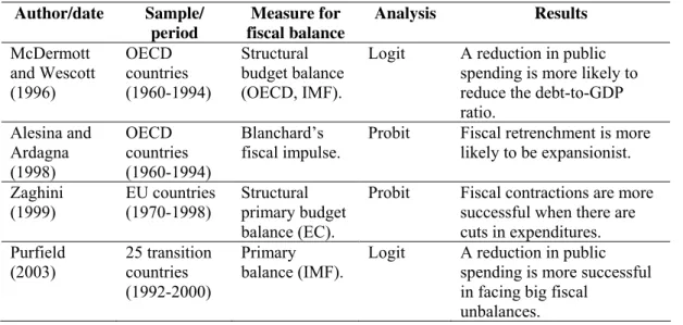
Table 2 – Empirical evidence on the success of fiscal consolidations

Author/date Sample/ period Measure for fiscal balance Analysis Results McDermott and Wescott (1996) OECD countries (1960-1994) Structural budget balance (OECD, IMF).

Logit A reduction in public spending is more likely to reduce the debt-to-GDP ratio. Alesina and Ardagna (1998) OECD countries (1960-1994) Blanchard’s fiscal impulse.

Probit Fiscal retrenchment is more likely to be expansionist.

Zaghini EU countries (1970-1998)

Structural primary budget balance (EC).

Probit Fiscal contractions are more successful when there are cuts in expenditures. Purfield (2003) 25 transition countries (1992-2000) Primary balance (IMF).

Logit A reduction in public spending is more successful in facing big fiscal

The abovementioned literature uses several definitions for identifying fiscal

consolidations, relying essentially on the structural budget balance concept, the

balance that would arise if both expenditures and taxes were determined by potential

rather than actual output. However, the structural budget does not allow the correction

of all the effects on budget balance resulting from changes in economic activity such

as inflation or real interest rate changes.

The usually adopted measure is the primary structural budget balance, i.e. the total

balance excluding interest expenditure. This measure is used either as percentage of

GDP or as a percentage of potential output. However, using the total budget balance

instead of the primary budget balance may have advantages, e.g. if the consolidation

leads to a lower interest rate and thus further consolidation benefits. In practice, and in

the surveyed studies, the differences between using the total budget deficit or the

primary budget deficit to determine the fiscal episodes are not very significant.

Besides the choice of the budget measure, there are also differences in the literature as

to how to define the period of a fiscal contraction or expansion. According to the

chosen definition, the number of fiscal episodes changes as well as the turning points

of fiscal policy (“trigger points” in Bertola and Drazen (1993) terminology).

For instance, Alesina and Perotti (1995) use two alternative definitions for fiscal

episodes: in the first one, they take into account the years where the change of the

primary structural balance exceeds 1.5 percent of GDP. In the second one, they

consider the years where the change of the primary structural balance deviates from

the country average change by plus or minus one standard deviation.

The definition used by Giavazzi and Pagano (1996) decreases the probability of fiscal

adjustment periods with only one year by using a limit of 3 percentage points of GDP

for a single year consolidation. They determine a fiscal adjustment by checking

whether the accumulated change in the primary structural deficit is above 5, 4 and 3

percentage points of GDP respectively in four, three and two consecutive years or the

change is of 3 percentage points of potential GDP in one single year. Alternatively,

Alesina and Ardagna (1998) adopted the following fiscal episode definition: the

or, increases 1.5 percentage points of GDP on average in two consecutive years. This

allows for instance that some stabilisation periods may have only one year.

3. Assessing fiscal adjustments

3.1. Determining fiscal episodes

We are interested in the evolution of the budget balance as a ratio of GDP, and also in

the fraction of that change that may be attributed to discretionary measures taken by

the fiscal authorities. In other words, we need to decompose the change of the budget

balance-to-GDP ratio into its components. In order to do that, one has to compute the

total derivative of the budget balance ratio.

Denoting the budget balance as B, which is equal to government revenues, T, minus

government expenditures, G, and being GDP given by Y, the total derivative of B/Y is

written as follows:

(

)

(

)

Y YdB

B Y dY

⎛

⎝⎜ ⎞⎠⎟ = + −⎛⎝⎜ ⎞⎠⎟ 1

2 (2)

d B Y dB Y B Y dY Y ⎛

⎝⎜ ⎞⎠⎟ = − , (3)

or, for small changes in the variables,

∆ B ∆ ∆

Y B Y B Y Y Y ⎛

⎝⎜ ⎞⎠⎟ = − . (4)

Defining b = B/Y, and since B=T-G, we can write

Y Y b Y G T

b= ∆ −∆ − ∆

Following for instance von Hagen et al. (2001) we can define a neutral fiscal policy

stance as resulting in identical changes in both government expenditures and

government revenues. This implies that we have ∆T=∆G in (5), which results in

Y Y b by ₌₋ ∆

∆ , (6)

where ∆by _{is then the contribution of economic growth to the change in the budget}

balance.3 This growth effect should now be deducted from the actual change in the

budget balance in order to proxy the discretionary change in the budget balance ∆b*_:

y

b b b =∆ −∆ ∆ *

. (7)

We can now proceed with the explanation of the criteria that we used to determine the

so-called fiscal consolidation events and the success of those events.

Our definition of an event, E, in period t, is as follows:

⎪⎩ ⎪ ⎨

⎧ _{∆ > +}

=

otherwise ,

0

] [

if ,

1 _t* µ γσ

t

b

E , (8)

where ∆b* _{was defined previously in (7), and µ and σ are respectively the average and}

the standard deviation for all discretionary changes in the budget balance in the entire

sample, while γ is applied to determine a multiple of the standard deviation as

commonly used in the literature.4

A fiscal adjustment is defined as successful if the general government balance

improves by α-times the standard deviation of all discretionary changes in the balance

3 _{Alternatively, one can notice that a more demanding definition, without assuming that ∆}

T=∆G, would imply a contribution of economic growth to the change in the budget balance given by

Y Y b t by = − ∆

∆ ( ) , where t=∆T/T and supposing also that ∆G=0.

4

for two consecutive years (rather like what was proposed by Alesina and Perotti (1995)): ⎪⎩ ⎪ ⎨ ⎧ > ∆ =

∑

SU , (9)

and we use, for simplicity, α=1 in (9).

In order to control for the composition of the adjustment, i. e. whether or not the

change in expenditure is significant vis-à-vis the change in the budget balance, we

construct the dummy variable EXP, to be used as an explanatory variable in the

subsequent Logit analysis. For the cases where a successful consolidation can be

found, variable EXP, as a percentage of GDP, is defined as follows

⎩ ⎨

⎧ ∆ ∆ > = otherwise , 0 ) / exp ( if ,

1 * _λ

t t t

b

EXP , (10)

where exp is the value for total expenditure in year t.

3.2. Descriptive data for fiscal episodes

As data sources the AMECO database of the EC is used for the EU15 countries, while

for the CE10 countries the WEO database is used.5 To have a view of how the

changes in discretionary fiscal balances are spread across countries and years, Figure

1 depicts the results of calculations for equation (7), using the total balance and λ=2/3

5 _{The relevant codes used for the data are as follows:}

Ameco WEO

- total budget deficit 1.0.319.0.UBLGE GGB - primary budget deficit 1.0.319.0.UBLGIE GGBXI - total expenditure 1.0.319.0.UUTGE GGENL - total revenue 1.0.319.0.URTG GGRG - interest expenditure 1.0.319.0.UYIGE GGEI

as our benchmark.6 As can be seen, the distribution is centred around zero and has a

higher kurtosis than the normal distribution.

Figure 1 – Changes in total “discretionary” balance,

CE10, and EU15, 1991-2003

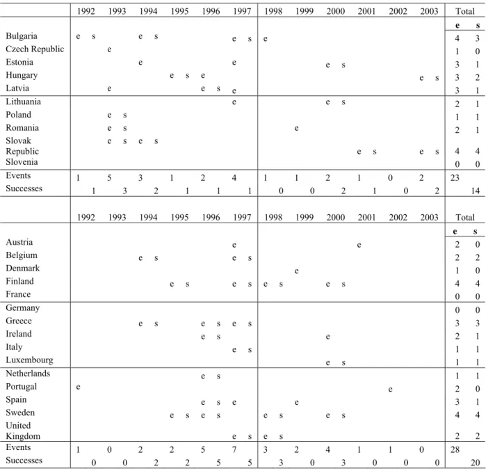
Moreover, Table 3 presents all the individual events identified for each country.

Almost all CE10 countries implemented fiscal consolidations according to our

definition during the first half of the nineties with 1993 being the year with the largest

number of consolidations. This might reflect that governments at that time used a

window of opportunity for fiscal consolidation as economic output bottomed out after

the drop in the early transition period and the growth outlook improved. Another

spike in the number of countries is 1997 with four observations after which the

number of events declines and remains equal or below two for the remainder of the

observation period. The only year where no fiscal consolidation is recorded in any of

the CE10 countries is 2002.7

By contrast, fiscal consolidations in the EU15 are concentrated in the years 1995

through 1997 with more than half of all observations occurring in this period. Another

6

For instance, McDermott and Westcott (1996) use a 60 per cent threshold. In section 4.2 we perform some sensitivity analysis to check the impact of changing our chosen threshold from 2/3 to 1/2 and to 3/4.

7

local maximum occurs in the year 2000 after which fiscal consolidation events are

rare and unsuccessful (cfr. lower panel of Table 3).8

Table 3 – Fiscal adjustment events and successes (using a 2/3 threshold), CE10, and EU15, 1991-2003

1992 1993 1994 1995 1996 1997 1998 1999 2000 2001 2002 2003 Total

e s

Bulgaria e s _{e s e s e 4 3}

Czech Republic _{e 1 0}

Estonia _{e e e s 3 1}

Hungary _{e s e e s 3 2}

Latvia _{e e s e 3 1}

Lithuania _{e e s 2 1}

Poland _{e s 1 1}

Romania _{e s e 2 1}

Slovak Republic

e s e s

e s e s 4 4

Slovenia _{0 0}

Events _{1 5 3 1 2 4 1 1 2 1 0 2 23}

Successes _{1 3 2 1 1 1 0 0 2 1 0 2 14}

1992 1993 1994 1995 1996 1997 1998 1999 2000 2001 2002 2003 Total

e s

Austria _{e e 2 0}

Belgium _{e s e s 2 2}

Denmark _{e 1 0}

Finland _{e s e s e s e s 4 4}

France _{0 0}

Germany _{0 0}

Greece _{e s e s e s 3 3}

Ireland _{e s e 2 1}

Italy _{e s 1 1}

Luxembourg _{e s 1 1}

Netherlands _{e s 1 1}

Portugal e _{e 2 0}

Spain _{e s e e 3 1}

Sweden _{e s e s e s e s 4 4}

United

Kingdom e s e s 2 2

Events _{1 0 2 2 5 7 3 2 4 1 1 0 28}

Successes _{0 0 2 2 5 5 3 0 3 0 0 0 20}

Note: e – event; s – success.

8

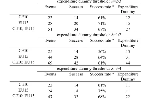
The number of events, successes and the occurrences of the expenditure dummy

composition are reported in Table 4 (also for alternative expenditure thresholds).9

With a less (more) demanding limit, one naturally gets more (less) fiscal events. For

instance, with a less demanding limit one also gets a few more successes and a

decrease in the success rate.

Table 4 – Events, successes and expenditure composition for the total balance

CE10 and EU15, 1991-2003

expenditure dummy threshold: λ=2/3

Events Success Success rate * Expenditure Dummy

CE10 _{23 14 61% 12}

EU15 _{28 20 71% 15}

CE10; EU15 _{51 34 67% 27}

expenditure dummy threshold: λ=1/2

Events Success Success rate * Expenditure Dummy

CE10 _{25 14 56% 13}

EU15 _{44 28 64% 31}

CE10; EU15 _{69 42 61% 44}

expenditure dummy threshold: λ=3/4

Events Success Success rate * Expenditure Dummy

CE10 _{23 14 61% 11}

EU15 _{24 18 75% 11}

CE10; EU15 _{47 32 68% 22}

Notes: The expenditure dummy means that there was a decrease in expenditures of at least λ

of the improvement in the budget balance, see (10). * - Successes/ Events.

3.3. Comparison of expenditure based adjustments

Table 5 presents some characteristics of different consolidations. There seems to be

some evidence that in Central and Eastern Europe expenditure based consolidations

tend to be somewhat larger than the average size of all consolidations. Similarly, it

would seem that Central and Eastern Europe expenditure based consolidations start

out from a higher overall deficit situation in the preceding year. With regard to the

growth rate in the period prior to the consolidation event, by contrast, there seems to

be no major difference.

9

Table 5 – Size of consolidations, total deficit

EU15 and CE10, 1991-2003

Size of consolidation (in % of GDP)

Average fiscal balance prior to consolidation

(in % of GDP)

Average growth prior to consolidation (in %) All

events

Expenditure based consolid.

All events

Expenditure based consolid.

All events

Expenditure based consolid. Total deficit

CE10 3.8 4.2 -6.4 -7.8 -1.6 -1.6

EU15 2.5 2.0 -3.9 -3.1 3.5 4.2

For the EU15 countries, the evidence is somewhat different since expenditure based

consolidations tend to be somewhat smaller than average (although the difference is

negligible when looking at primary deficits). Also in contrast to Central and Eastern

Europe, expenditure based consolidations tend to start out from lower deficits and

higher growth rates in the preceding period.

Overall, this evidence would support the notion that expenditure based consolidations

are perceived differently by policy makers in Central and Eastern Europe and in the

EU15. In Central and Eastern Europe expenditure based consolidations may be seen

as a more drastic tool for consolidation in times of greater fiscal distress. Conversely,

in the EU15, expenditure reduction might be perceived as more of a fiscal “luxury”

that can be implemented in times of stronger growth and less pressing consolidation

requirements. One possible explanation for the different perceptions could lie in

different administrative capacity between the two country groups. While generally

well developed tax administrations in the EU15 allowed those countries to implement

revenue increases in times of consolidation, a lack of such capacity may have driven

the Central Eastern European countries to resort to expenditure reductions during the

observation period. The importance of administrative capacity for the development of

fiscal policies those countries has been highlighted by Purfield (2003) and Gupta et al.

4. Analytical framework

4.1. Estimation results and discussion

In this section we assess whether the relative share of expenditure changes in the

consolidation affects the success of fiscal consolidations. To answer those questions a

Logit model was estimated, defining

[

]

1 , (11)

where E[S=1|Zi] is the conditional expectation of the success of a fiscal

consolidation, given Zi, with

⎩ ⎨ ⎧ = ; , 0 , , 1 successful not is ion consolidat the if successful is ion consolidat the if

S , (12)

One can interpret (11) as the conditional probability that a successful consolidation

occurs given Zi, and

i i

i B EXP

Z =

α

β

δ

where B is the “discretionary change” in the primary budget balance (computed via

(7)). The dummy variable EXP was defined in (10), and assumes the value one when

the change in the primary expenditure is at least two thirds of the change in the

primary budget balance, and zero otherwise.

In order to assess whether there is a different behaviour between the EU15 countries

and the CE10 countries, the following modified version of (13) was also estimated:

) (

) ( )

( _{1 2 i 1 i 2 i i 1 i 2 i i}

i D B D B EXP D EXP

Z = α +α + β + β +δ +δ , (14)

where D is a dummy variable that takes the value one if a country belongs to the

the other hand, α2 is the difference to the intercept and β2 and δ2 are the slope

differences of one group of countries vis-à-vis the other group.

The results for the estimation of equations (13) and (14) are reported in Table 6, using

the total budget balance.

Table 6 – Estimation results (using a 2/3 threshold) for total balances,

EU15 and CE10, 1991-2003

EU15, CE10 No group

dummy, eq. (13)

With group dummy, eq. (14)

EU15

eq. (13)

CE10

eq. (13)

α (constant) -2,48 ** (-2,09)

-2,97 (-1,44)

-3,11 * (-1,87)

α1 -3,11 *

(-1,87)

α2 0,14 *

(2,65)

β (B) 0,83 ** (2,15)

1,42 *

(1,75)

0,60 (1,33)

β1 0,60

(1,33)

β2 0,82

(0,88)

δ (EXP) 1,89 *** (2,57)

1,19 (1,18)

3,38 ** (2,52)

δ1 3,38 **

(2,52)

δ2 -2,20

(-1,31)

McFadden R2 0,29 0,30 0,14 0,48

Nº of observations 51 51 28 23

dP/dZ: B 0,14 0.09

0.12

0,24 0,06

EXP 0,32 0.48

-0.31

0,20 0,36

Notes: The t statistics are in brackets. *, **, *** - Significant at the 10, 5 and 1 per cent level respectively. The effect in the probability of success from a change in a continuous variable Z, is approximated by dP/dZ ≅β[P_i(1−P_i)].

Table 6 (first column) shows that the size of the discretionary change in total balance

is statistically significant to explain the success of a fiscal consolidation, and this has

the expected sign. This means, the larger the size of the initial fiscal adjustment, the

higher is the probability that the improvement will last over two periods. However,

that effect is not significant when only the CE10 country group is considered (last

For the CE10 sub-set of countries, only the dummy variable, EXP, that reflects the

size of change in expenditures relative to the change in the total budget balance, is

significant. In other words, for the CE countries the composition of the adjustment

seems relevant – expenditure-based adjustments have a higher probability to

succeed.10

The advantage of the dummy variable approach (i. e. estimating the pooled equation

(14)) is that one gets more insights than by just doing a simple Chow test (i. e.

estimating equation (13) for the three sub-samples). Indeed, from Table 6, the fact that

the differential intercept coefficient α2 is statistically significant, allows accepting that

the separate regressions for the EU15 and CE10 countries have a different intercept.

Moreover, one can also see that the differential slope for the expenditure dummy is

statistically different between the two groups of countries.

Given that the results using the expenditure dummy are not entirely unambiguous the

results from the opposite approach may be instructive. In particular, instead of

including an expenditure dummy in the regression we include a revenue dummy,

which is defined in the analogous way:

⎩ ⎨

⎧ ∆ ∆ > =

otherwise ,

0

) / ( if ,

1 t t* λ

t

b rev

REV . (15)

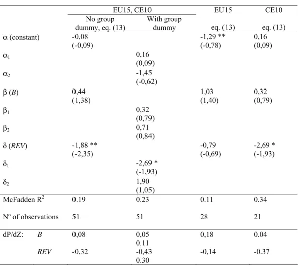
In line with our expectations, Table 7 (also with λ=2/3 in (15)) reveals that the

presence of the revenue dummy in the estimation has a significantly negative impact

on the likelihood of a successful consolidation. The details of the table reveal that this

effect is driven by the behaviour of the CE10, whereas the dummy remains

insignificant for the EU15. This result supports the notion discussed above, that tax

increases in the CE10 are less likely to contribute to sustainable fiscal consolidation.

10

Table 7 – Estimation results (using a 2/3 threshold) for total balances and with revenue dummy, EU15 and CE10, 1991-2003

EU15, CE10

No group With group dummy

EU15 CE10

α (constant) -0,08 (-0,09)

-1,29 **

(-0,78)

0,16 (0,09)

α1 0,16

(0,09)

α2 -1,45

(-0,62)

β (B) 0,44

(1,38)

1,03 (1,40)

0,32 (0,79)

β1 0,32

(0,79)

β2 0,71

(0,84)

δ (REV) -1,88 ** (-2,35)

-0,79 (-0,69)

-2,69 * (-1,93)

δ1 -2,69 *

(-1,93)

δ2 1,90

(1,05)

McFadden R2 0.19 0.23 0.11 0.34

Nº of observations 51 51 28 21

dP/dZ: B 0,08 0,05

0.11

0,18 0.04

REV -0,32 -0,43

0.30

-0,14 -0.37

Notes: The t statistics are in brackets. *, **, *** - Significant at the 10, 5 and 1 per cent level respectively. The effect in the probability of success from a change in a continuous variable Z, is approximated by dP/dZ ≅β[P_i(1−P_i)].

4.2. Alternative specifications

To test for the robustness of the reported results, we tried several alternative

approaches of our model. All in all, the results presented in the following show that

these alternatives seem to give some robustness to the results reported for

specifications initially chosen.

First we tested an alternative approach for the expenditure dummy variable in (10).

Instead of checking for the change of public expenditure in relation to the

improvement of the budget balance, one can be more lenient and take into account the

cumulative change of both period t and period t-1. For instance, and for the cases

where a successful consolidation can be found, a variable EXPDUR, as a percentage

of GDP, can be defined as follows

⎪⎩ ⎪ ⎨ ⎧

> ∆ ∆

=

∑

− −

otherwise ,

0

) / exp (

if , 1

1

0

* _λ

i

i t i t t

b

EXPDUR , (16)

where exp is still the value for total expenditure in year t.

Therefore, specifications (13) and (14) can be estimated as equations (13’) and (14’)

using the alternative dummy expenditure duration variable. These results are

presented in the Appendix B.

For the total balance, our results seem to indicate that a more durable

expenditure-based adjustment is more relevant in explaining the success of fiscal consolidations in

the CE10 countries than in the EU15 countries. Indeed, it can be seen that the

differential slope for the duration expenditure dummy, δ2, is statistically different

between the two groups of countries. Since the two regressions have, statistically

speaking, the same intercept, but different slopes, we may assume that these two

concurrent regressions do portray different reaction functions for the EU15 and for the

CE10 countries. In other words, the idea of some persistence of an expenditure-based

adjustment seemed to be more relevant in explaining the success of fiscal

consolidations in the CE10 countries than in the EU15 countries.

Additionally, the general specification (13) was also used with a multiplicative

expenditure dummy instead of an additive dummy, that is,

)

( _{i i}

i

i B EXP B

Z = α + β +δ × . (17)

However, the estimation results for (17) were rather similar to the ones already

obtained with the additive expenditure dummy, without any relevant gains in terms of

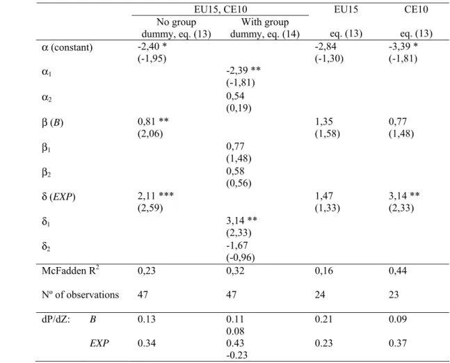
Some sensitivity analysis was performed in order to assess whether changing the 2/3

threshold for the setting up of the fiscal events, the γ factor in equation (8), and also

for the attribution of values to the dummy expenditure variable in (10), would

impinge significantly on the results. Alternative thresholds 1/2 and 3/4 were then

used, and the results reported respectively in Tables 8 and 9, are rather similar to the

ones already presented for the initial case with the 2/3 threshold.

Table 8 – Estimation results (using a 1/2 threshold) for total balances,

EU15 and CE10, 1991-2003

EU15, CE10 No group

dummy, eq. (13)

With group dummy, eq. (14)

EU15

eq. (13)

CE10

eq. (13)

α (constant) -1,63 ** (-2,25)

-1,45 (-1,30)

-2,97 ** (-2,16)

α1 -2,97 **

(-2,16)

α2 1,52

(0,86)

β (B) 0,59 ** (2,22)

1,05 *

(1,90)

0,58 (1,50)

β1 0,58

(1,50)

β2 0,47

(0,69)

δ (EXP) 1,06 * (1,91)

0,00 (0,01)

2,54 ** (2,24)

δ1 2,54 **

(2,24)

δ2 -2,53 *

(-1,88)

McFadden R2 0,14 0,22 0,10 0,51

Nº of observations 69 69 44 25

dP/dZ: B 0.12 0.10

0.08

0.22 0.07

EXP 0.21 0.45

-0.45

0.00 0.32

Notes: The t statistics are in brackets. *, **, *** - Significant at the 10, 5 and 1 per cent level respectively. The effect in the probability of success from a change in a continuous variable Z, is approximated by dP/dZ ≅β[P_i(1−P_i)].

Additional control variables such as GDP real growth rate and inflation were used

under several alternative specifications of the Logit model. However, results were not

improved.

We also allowed for a longer time lag for assessing the success of a consolidation

evaluate the success, or not, of the effort. In other words, instead of using two

consecutive years in the determination of the successes in (9), we used three

consecutive years. Nevertheless, and since the resulting dummy variable is highly

correlated with the one we already used (correlation is around 0.90), the results were

broadly unchanged. Moreover, there was even a small decrease in the number of

successes since in some cases, to apply this longer span, an additional observation

would be needed.11

Table 9 – Estimation results (using a 3/4 threshold) for total balances,

EU15 and CE10, 1991-2003

EU15, CE10 No group

dummy, eq. (13)

With group dummy, eq. (14)

EU15

eq. (13)

CE10

eq. (13)

α (constant) -2,40 * (-1,95)

-2,84 (-1,30)

-3,39 * (-1,81)

α1 -2,39 **

(-1,81)

α2 0,54

(0,19)

β (B) 0,81 ** (2,06)

1,35 (1,58)

0,77 (1,48)

β1 0,77

(1,48)

β2 0,58

(0,56)

δ (EXP) 2,11 *** (2,59)

1,47 (1,33)

3,14 ** (2,33)

δ1 3,14 **

(2,33)

δ2 -1,67

(-0,96)

McFadden R2 0,23 0,32 0,16 0,44

Nº of observations 47 47 24 23

dP/dZ: B 0.13 0.11

0.08

0.21 0.09

EXP 0.34 0.43

-0.23

0.23 0.37

Notes: The t statistics are in brackets. *, **, *** - Significant at the 10, 5 and 1 per cent level respectively. The effect in the probability of success from a change in a continuous variable Z, is approximated by dP/dZ ≅β[P_i(1−P_i)].

11

Finally, instead of using a dummy variable to capture the dimension of the change in

expenditures vis-à-vis de improvement of the budget balance, we used the change

itself, namely for the 2/3 threshold for the expenditure dummy variable. Again there

was no enhancement in the results, which were also in line with the results already

presented, but now with lower statistical significance. All in all, these alternative

approaches seem to give some robustness to the results reported for our initially

chosen specification.

Table 10 summarises the several sets of results for the alternative limits, and one can

notice that with the 1/2 threshold the expenditure dummy variable also becomes

significantly different from zero for the group of EU15 countries when the primary

balance is used.

The evidence regarding expenditure-based adjustments is weak for the EU15 country

group, also compared to the literature presented above. Here, one has to bear in mind

that due to the limited available data for the CEE country group, starting only in 1991,

this implies excluding from the sample a significant number of consolidations that

occurred in the 1980s and before in the EU15 countries. On the other hand, the limited

time span precludes using longer periods to assess the successes, as already mentioned

Table 10 – Summary of statistical significance findings

Total balance Primary balance

EU15, CE10

EU15 CE10 EU15,

CE10

EU15 CE10

Expenditures (revenues) decrease (increase) by at least 2/3 of the improvement in the budget balance

“discretionary change”

β (B) yes yes no yes yes yes

Expenditure dummy

δ (EXP) yes no yes yes* no no

Revenue dummy

δ (REV) yes no yes no no no

Expenditures (revenues) decrease (increase) by at least 1/2 of the improvement in the budget balance

“discretionary change”

β (B) yes yes no yes yes yes

Expenditure dummy

δ (EXP) yes no yes no yes no

Revenue dummy

δ (REV) yes no yes no no no

Expenditures (revenues) decrease (increase) by at least 3/4 of the improvement in the budget balance

“discretionary change”

β (B) yes no no yes yes yes

Expenditure dummy

δ (EXP) yes no yes yes no no

Revenue dummy

δ (REV) yes no yes no no no

Note: the full set of results for the revenue dummy with the alternative thresholds of 1/2 and 3/4 are not reported in the paper, but are available from the authors on request.

* After accounting for border line cases: Bulgaria 1994 and Finland 1994.

5. Conclusion

Many of the CE10 countries will have to undertake fiscal consolidation in the near

future to reverse the trend of rising debt ratios and comply with the EU fiscal

framework. Thus the question of how to design fiscal consolidations is of imminent

interest.

The theoretical and empirical literature shows that basing fiscal consolidation on

expenditure reduction can have beneficial macroeconomic effects and raise the

probability of success. However, conclusive evidence for the CE10 has so far been

This paper shows that since the early 1990’s expenditure based consolidations have

indeed tended to be more successful in Central and Eastern Europe. The reverse is

also true, namely that revenue based consolidations have tended to reduce the

likelihood of success. The results are robust to alternative thresholds for the

identification of fiscal events and the composition dummies. Using primary balances

we find some support for a significant role of the expenditure dummy when

estimating the effect for the EU15 and the CE10 combined, but not at the

disaggregated level.

The results differ from those for the EU15 countries, where both composition

dummies remain generally insignificant. The dominance of expenditure based

consolidations in Central and Eastern Europe could be explained by an inability to

increase revenue ratios above already high levels due to a lack of administrative

Appendix A – Primary balance results

Table A1 – Fiscal adjustment events and successes (using a 2/3 threshold), primary balance, CE10, and EU15, 1991-2003

1992 1993 1994 1995 1996 1997 1998 1999 2000 2001 2002 2003 Total

e s

Bulgaria _{e s 1 1}

Czech Republic _{0 0}

Estonia _{e e s 2 1}

Hungary _{e s e s e s e s 4 4}

Latvia _{e e s e s e 4 2}

Lithuania _{e e s 2 1}

Poland _{e s 1 1}

Romania _{e s e e 3 1}

Slovak

Republic

e s e s

e e 4 2

Slovenia _{0 0}

Events _{0 4 3 2 2 4 0 1 2 1 0 2 21}

Successes _{0 3 3 2 2 0 0 0 2 0 0 1 13}

1992 1993 1994 1995 1996 1997 1998 1999 2000 2001 2002 2003 Total

e s

Austria _{e e 2 0}

Belgium _{e 1 0}

Denmark _{e 1 0}

Finland _{e s e s e e s 4 3}

France _{e 1 0}

Germany _{0 0}

Greece _{e s e s 2 2}

Ireland _{e e 2 0}

Italy e _{e e 3 0}

Luxembourg _{e e s 2 1}

Netherlands _{e 1 0}

Portugal e _{e 2 0}

Spain _{e 1 0}

Sweden _{e s e s e s e e 5 3}

United

Kingdom e s e s e 3 2

Events _{2 0 4 2 7 5 3 1 4 1 1 0 30}

Successes _{0 0 3 1 3 2 0 0 2 0 0 0 11}

Table A2 – Events, successes and expenditure composition, primary balance,

CE10, and EU15, 1991-2003

expenditure dummy threshold: λ=2/3

Events Success Success rate * Expenditure Dummy

CE10 _{21 13 62% 12}

EU15 _{30 11 37% 15}

CE10; EU15 _{51 24 47% 27}

expenditure dummy threshold: λ=1/2

Events Success Success rate * Expenditure Dummy

CE10 _{24 14 58% 15}

EU15 _{48 12 25% 28}

CE10; EU15 _{72 26 36% 43}

expenditure dummy threshold: λ=3/4

Events Success Success rate * Expenditure Dummy

CE10 _{20 12 60% 11}

EU15 _{27 11 41% 11}

CE10; EU15 _{47 23 49% 22}

Table A3 – Estimation results (using a 2/3 threshold) for primary balances,

EU15 and CE10, 1991-2003

EU15, CE10 No group

dummy, eq. (13)

With group dummy, eq. (14)

EU15

eq. (13)

CE10

eq. (13)

α (constant) -3,82 *** (-3,23)

-4,06 **

(-2,36)

-3,54 * (-1,89)

α1 -3,54 *

(-1,89)

α2 -0,52

(-0,20)

β (B) 1,24 *** (2,98)

1,37 **

(2,03)

1,10 * (1,87)

β1 1,10 *

(1,87)

β2 0,27

(0,30)

δ (EXP) 0,86 (1,23)

0,77 (0,86)

1,07 (0,95)

δ1 1,07

(0,95)

δ2 -0,30

(-0,21)

McFadden R2 0,27 0,28 0,19 0,32

Nº of observations 51 51 30 21

dP/dZ: B 0,21 0.18

0.04

0,24 0,17

EXP 0,14 0.18

0.05

0,14 0,16

Table A4 – Estimation results (using a 1/2 threshold) for primary balances,

EU15 and CE10, 1991-2003

EU15, CE10 No group

dummy, eq. (13)

With group dummy, eq. (14)

EU15

eq. (13)

CE10

eq. (13)

α (constant) -4,00 *** (-4,25)

-5,76 ***

(-3,09)

-2,50 * (-1,94)

α1 -2,50 *

(-1,94)

α2 -3,27

(-1,44)

β (B) 1,24 *** (3,43)

1,51 **

(2,20)

1,03 ** (2,15)

β1 1,03 **

(2,15)

β2 0,48

(0,58)

δ (EXP) 0,91 (1,38)

2,27 *

(1,91)

-0,32 (-0,30)

δ1 -0,32

(-0,30)

δ2 2,59

(1,62)

McFadden R2 0,32 0,36 0,33 0,27

Nº of observations 72 72 48 24

dP/dZ: B 0.18 0.14

0.07

0.18 0.17

EXP 0.13 -0.04

0.35

0.28 -0.05

Table A5 – Estimation results (using a 3/4 threshold) for primary balances,

EU15 and CE10, 1991-2003

EU15, CE10 No group

dummy, eq. (13)

With group dummy, eq. (14)

EU15

eq. (13)

CE10

eq. (13)

α (constant) -4,52 *** (-3,24)

-3,87 **

(-2,26)

-7,59 ** (-1,98)

α1 -7,58 **

(-1,98)

α2 3,72

(0,89)

β (B) 1,41 *** (3,01)

1,28 **

(1,98)

2,15 * (1,95)

β1 2,15 *

(1,95)

β2 -0,87

(-0,68)

δ (EXP) 1,38 * (1,77)

1,08 (1,16)

2,43 (1,41)

δ1 2,43

(1,41)

δ2 -1,34

(-0,69)

McFadden R2 0,32 0,38 0,17 0,52

Nº of observations 47 47 27 20

dP/dZ: B 0.22 0.32

-0.13

0.24 0.23

EXP 0.22 0.37

-0.21

0.20 0.25

Appendix B – Expenditure duration dummy results

Table B1. Estimation results, expenditure duration dummy (using a 2/3 threshold) for total balances, EU15 and CE10, 1991-2003

EU15, CE10 No group

dummy, eq. (13’)

With group dummy, eq. (14’)

EU15

eq. (13’)

CE10

eq. (13’)

α (constant) -1.36 (-1.48)

-0.67 (-0.37)

-3.2 ** (-1.99)

α1 -3.2 **

(1.99)

α2 2.5

(1.03)

β (B) 0.56 *

(1.83)

1.15 (1.54)

0.55

(1.54)

β1 0.55

(1.54)

β2 0.59

(0.72)

δ (EXPDUR) 0.70 (1.03)

-1.29 (-1.06)

2.57 ** (2.07)

δ1 2.57 **

(2.07)

δ2 -3.86 **

(-2.22)

McFadden R2 0.11 0.25 0.14 0.35

Nº of observations 51 51 28 23

dP/dZ: B 0.11 0.09

0.09

0.20 0.08

EXPDUR 0.14 0.40

-0.60

-0.22 0.35

Table B2. Estimation results, expenditure duration dummy (using a 2/3 threshold) for primary balances, EU15 and CE10, 1991-2003

EU15, CE10 No group

dummy, eq. (13’)

With group dummy, eq. (14’)

EU15

eq. (13’)

CE10

eq. (13’)

α (constant) -3.52 *** (-3.25)

-3.43 ** -3.86 ** (-2.04)

α1 -3.86 **

(-2.04)

α2 0.43

(0.17

β (B) 1.16 *** (2.98)

1.25 **

(1.97)

1.00 * (1.84)

β1 1.00

(1.83)

β2 0.25

(0.30)

δ (EXPDUR) 0.52 (0.74)

0.04 (0.05)

1.61 (1.22)

δ1 1.61

(1.22)

δ2 -1.57

(-0.99)

McFadden R2 0.31 0.28 0.17 0,34

Nº of observations 51 51 30 21

F Test 0,19 $

dP/dZ: B 0.20 0.17

0.04

0.23 0.14

EXPDUR 0.09 0.27

-0.26

0.01 0.23

References

Afonso, A. (2001). “Non-Keynesian Effects of Fiscal Policy in the EU-15,” ISEG/UTL – Technical University of Lisbon, Economics Department Working Paper nº 07/2001/DE/CISEP.

Alesina, A. and Ardagna, S. (1998). “Tales of Fiscal Contractions,” Economic Policy, 27, 487-545.

Alesina, A. and Perotti, R. (1995). “Fiscal Expansions and Adjustments in OECD countries,” Economic Policy, 21, 205-248.

Alesina, A. and Perotti, R. (1997). “Fiscal Adjustments in OECD countries: Composition and Macroeconomic Effects,” International Monetary Fund Staff Papers, 44 (2), 210-248.

Backé, P.; Thimann, C.; Arratibel, O.; Calvo-Gonzalez, O.; Mehl, A. and Nerlich, C. (2004). “The acceding countries’ strategies towards ERM II and the adoption of the euro: an analytical review,” ECB Occasional Paper 10.

Bertola, G. and Drazen, A. (1993). "Trigger Points and Budget Cuts: Explaining the Effects of Fiscal Austerity," American Economic Review, 83 (1), 11-26.

Blanchard, O. and Perotti, R. (2002). “An empirical characterization of the dynamic effects of changes in government spending and taxes on output,” Quarterly Journal of Economics, 117 (4), 1329-1368.

De Arcangelis, G. and Lamartina, S. (2003). “Identifying fiscal shocks and policy regimes in OECD countries”, ECB Working Paper 281.

EC (2003). Public Finances in EMU, European Commission.

Frenkel, M. and Nickel, C. (2005). “Shocks and shock adjustment dynamics in the euro area and the CEECs,“ Journal of Common Market Studies, 43 (1), 53-74.

Giavazzi, F. and Pagano, M. (1990). “Can Severe Fiscal Contractions be Expansionary? Tales of Two Small European Countries,” in Blanchard, O. and Fischer, S. (eds.), NBER Macroeconomics Annual 1990, MIT Press.

Giavazzi, F. and Pagano, M. (1996). “Non-keynesian Effects of Fiscal Policy Changes: International Evidence and the Swedish Experience,” Swedish Economic Policy Review, 3 (1), 67-103.

Giavazzi, F.; Jappelli, T. and Pagano, M. (2000). “Searching for non-linear effects of fiscal policy: evidence from industrial and developing countries,” European Economic Review, 44 (7), 1259-1289.

Gupta, S.; Leruth, L.; de Mello, L. and Chakravarti, S. (2001). “Transition Economies:

Hjelm, G. (2002). “Is private consumption growth higher (lower) during periods of fiscal contractions (expansions)?” Journal of Macroeconomics 24 (1), 17-39.

Heylen, F. and Everaert, G. (2000). “Success and Failure of Fiscal Consolidation in the OECD: A Multivariate Analysis,” Public Choice, 105 (1/2), 103-124.

McDermott, C. and Wescott, R. (1996). “An Empirical Analysis of Fiscal Adjustments,” International Monetary Fund Staff Papers, 43 (4), 725-753.

Perotti, R. (1998). “The Political Economy of Fiscal Consolidations,” Scandinavian Journal of Economics, 100 (1) 367-394.

Purfield, C. (2003). “Fiscal Adjustment in Transition Countries: Evidence from the 1990s,” IMF Working Paper N. WP/03/36.

Sousa, L. and Borbély, D. (2003). “A Primer on Budgetary Questions on the New EU Members States,” mimeo, Kiel Institute for World Economics (IfW).

Tondl, G. (2004). “Macroeconomic effects of fiscal policies in the acceding countries,” Vienna University of Economics, April, mimeo.

fiscal policy changes? The EMU case,” Journal of Macroeconomics 25 (2), 213-240.

Zaghini, A. (1999). “The Economic Policy of Fiscal Conditions: The European Experience,” Banca d' Italia, Temi di Discussione, nº 355, June.

van Aarle, B. and Garretsen, H. (2003). “Keynesian, non-Keynesian or no effects of

EMU,” European Commission, Economic Papers n. 148, March.

European Central Bank working paper series

For a complete list of Working Papers published by the ECB, please visit the ECB’s website (http://www.ecb.int)

425 “Geographic versus industry diversification: constraints matter” by P. Ehling and S. B. Ramos, January 2005.

426 “Security fungibility and the cost of capital: evidence from global bonds” by D. P. Miller and J. J. Puthenpurackal, January 2005.

427 “Interlinking securities settlement systems: a strategic commitment?” by K. Kauko, January 2005.

428 “Who benefits from IPO underpricing? Evidence form hybrid bookbuilding offerings” by V. Pons-Sanz, January 2005.

429 “Cross-border diversification in bank asset portfolios” by C. M. Buch, J. C. Driscoll and C. Ostergaard, January 2005.

430 “Public policy and the creation of active venture capital markets” by M. Da Rin, G. Nicodano and A. Sembenelli, January 2005.

431 “Regulation of multinational banks: a theoretical inquiry” by G. Calzolari and G. Loranth, January 2005.

432 “Trading european sovereign bonds: the microstructure of the MTS trading platforms” by Y. C. Cheung, F. de Jong and B. Rindi, January 2005.

433 “Implementing the stability and growth pact: enforcement and procedural flexibility” by R. M. W. J. Beetsma and X. Debrun, January 2005.

434 “Interest rates and output in the long-run” by Y. Aksoy and M. A. León-Ledesma, January 2005.

435 “Reforming public expenditure in industrialised countries: are there trade-offs?” by L. Schuknecht and V. Tanzi, February 2005.

436 “Measuring market and inflation risk premia in France and in Germany” by L. Cappiello and S. Guéné, February 2005.

437 “What drives international bank flows? Politics, institutions and other determinants” by E. Papaioannou, February 2005.

438 “Quality of public finances and growth” by A. Afonso, W. Ebert, L. Schuknecht and M. Thöne, February 2005.

439 “A look at intraday frictions in the euro area overnight deposit market” by V. Brousseau and A. Manzanares, February 2005.

440 “Estimating and analysing currency options implied risk-neutral density functions for the largest new EU member states” by O. Castrén, February 2005.

441 “The Phillips curve and long-term unemployment” by R. Llaudes, February 2005.

442 “Why do financial systems differ? History matters” by C. Monnet and E. Quintin, February 2005.

443 “Explaining cross-border large-value payment flows: evidence from TARGET and EURO1 data” by S. Rosati and S. Secola, February 2005.

444 “Keeping up with the Joneses, reference dependence, and equilibrium indeterminacy” by L. Stracca and Ali al-Nowaihi, February 2005.

446 “Trade effects of the euro: evidence from sectoral data” by R. Baldwin, F. Skudelny and D. Taglioni, February 2005.

447 “Foreign exchange option and returns based correlation forecasts: evaluation and two applications” by O. Castrén and S. Mazzotta, February 2005.

448 “Price-setting behaviour in Belgium: what can be learned from an ad hoc survey?” by L. Aucremanne and M. Druant, March 2005.

449 “Consumer price behaviour in Italy: evidence from micro CPI data” by G. Veronese, S. Fabiani, A. Gattulli and R. Sabbatini, March 2005.

450 “Using mean reversion as a measure of persistence” by D. Dias and C. R. Marques, March 2005.

451 “Breaks in the mean of inflation: how they happen and what to do with them” by S. Corvoisier and B. Mojon, March 2005.

452 “Stocks, bonds, money markets and exchange rates: measuring international financial transmission” by M. Ehrmann, M. Fratzscher and R. Rigobon, March 2005.

453 “Does product market competition reduce inflation? Evidence from EU countries and sectors” by M. Przybyla and M. Roma, March 2005.

454 “European women: why do(n’t) they work?” by V. Genre, R. G. Salvador and A. Lamo, March 2005.

455 “Central bank transparency and private information in a dynamic macroeconomic model” by J. G. Pearlman, March 2005.

456 “The French block of the ESCB multi-country model” by F. Boissay and J.-P. Villetelle, March 2005.

457 “Transparency, disclosure and the federal reserve” by M. Ehrmann and M. Fratzscher, March 2005.

458 “Money demand and macroeconomic stability revisited” by A. Schabert and C. Stoltenberg, March 2005.

459 “Capital flows and the US ‘New Economy’: consumption smoothing and risk exposure” by M. Miller, O. Castrén and L. Zhang, March 2005.

460 “Part-time work in EU countries: labour market mobility, entry and exit” by H. Buddelmeyer, G. Mourre and M. Ward, March 2005.

461 “Do decreasing hazard functions for price changes make any sense?” by L. J. Álvarez, P. Burriel and I. Hernando, March 2005.

462 “Time-dependent versus state-dependent pricing: a panel data approach to the determinants of Belgian consumer price changes” by L. Aucremanne and E. Dhyne, March 2005.

463 “Break in the mean and persistence of inflation: a sectoral analysis of French CPI” by L. Bilke, March 2005.

464 “The price-setting behavior of Austrian firms: some survey evidence” by C. Kwapil, J. Baumgartner and J. Scharler, March 2005.

465 “Determinants and consequences of the unification of dual-class shares” by A. Pajuste, March 2005.

466 “Regulated and services’ prices and inflation persistence” by P. Lünnemann and T. Y. Mathä, April 2005.

467 “Socio-economic development and fiscal policy: lessons from the cohesion countries for the new member states” by A. N. Mehrotra and T. A. Peltonen, April 2005.

469 “Money and prices in models of bounded rationality in high inflation economies” by A. Marcet and J. P. Nicolini, April 2005.

470 “Structural filters for monetary analysis: the inflationary movements of money in the euro area” by A. Bruggeman, G. Camba-Méndez, B. Fischer and J. Sousa, April 2005.

471

April 2005.

472 “Yield curve prediction for the strategic investor” by C. Bernadell, J. Coche and K. Nyholm, April 2005.

473 “Fiscal consolidations in the Central and Eastern European countries” by A. Afonso, C. Nickel “Real wages and local unemployment in the euro area” by A. Sanz de Galdeano and J. Turunen,