A NALYSIS OF NEW TECHNIQUES FORR

(1)

MASTER OF SCIENCE IN

A

CTUARIAL

S

CIENCE

MASTERS FINAL WORK

D

ISSERTATION

ANALYSIS OF NEW TECHNIQUES FOR RISK AGGREGATION AND

DEPENDENCE MODELLING

(2)

MASTER OF SCIENCE IN

A

CTUARIAL

S

CIENCE

MASTERS FINAL WORK

D

ISSERTATION

ANALYSIS OF NEW TECHNIQUES FOR RISK AGGREGATION AND

DEPENDENCE MODELLING

M

OSTAFA

S

HAMS

E

SFAND

A

BADI

S

UPERVISOR

:

P

ROF

.

D

R

M

ARIA DE

L

OURDES

C

ENTENO

(3)

Abstract

In risk aggregation we are interested in the distribution of the sum of dependent risks. The objective of risk aggregation and dependence modeling is to model adequately dependent in-surance portfolios in order to evaluate the overall risk exposure. This master thesis investigates some practical aspects of modeling risk aggregation and dependency. We give an introduction

tocopula-based hierarchical aggregation model through reordering algorithm. This approach can

(4)

Acknowledgements

(5)

1. Introduction

Dependence modelling can not be ignored. This motivated me to write my master’s thesis in this field. The 2008 financial crisis have shown that the modelling dependence between risks is necessary for prudent risk aggregation. Most regulatory frameworks such as Solvency II need such a dependence modelling. I am interested in new risk aggregation techniques in this thesis and I will focus on practical aspects of modelling risk aggregation and dependency. From a practical point of view, copula-based hierarchical model through reordering algorithm is a flexible approach proposed for risk aggregation. My master’s thesis is inspired by the work of Dr. Philipp Arbenz, especially his paper on Copula based hierarchical risk aggregation through

sample reordering(see Arbenz et al. [2012]) and his PhD thesis (see Arbenz [2012]). To illustrate

hierarchical aggregation method empirically, we apply this approach to Danish Fire Insurance

Data. I use the statistical software packageR many times in my thesis.

(7)

2. Multivariate Models

Life is full of risks. Probability Theory as a special language is being applied to the area of risk modeling. Risks represented by random variables mapping unpredictable future events into actual amounts standing for profits and losses. In this thesis we are interested in aggregate risks as the overall risk or the risk of a portfolio. Risk aggregation is the aggregation of individual risks using a model for aggregation. Different methods for risk aggregation can be considered in practice. A good aggregation model is providing at the same time both probabilistic descriptions of individual risks and of their dependence or correlation structure.

A multivariate model has many applications in insurance mathematics and one of its most important application is risk aggregation model. A multivariate model for risks in the form of a joint cdf, survival function or density allows us to understand and approximate the unknown true joint distribution anddependence structure among the risks. There are many methods for modeling multivariate risks and their dependencies. Depending on the available input and the required output and constraints such as regulatory rules, different multivariate models can be selected. In this chapter and next chapter, briefly we talk about multivariate models and we explain basically three popular multivariate models for risk aggregation (see Arbenz [2012]);

• variance-covariance method

• risk factor models

• copula models

LetXi: Ω→Rfori∈Ndenote individual risks describing values of losses or gains. Assume

we are exposed tod risks X = (X1, ..., Xd). In this case, our interest is the distribution of the

random vector;

(X1, ..., Xd) : Ω→Rd

The marginal cdf of individual risk Xi, Fi(x) =P(Xi ≤x), does not have any information on

dependence structure and it is only characterizing the stochasticity of the single riskXi. We call FX(x) the joint cdf of the random vector of risks X = (X1, ..., Xd). When we fix the joint cdf FX(x), we state a multivariate model containing the all marginal behaviour distributions and

the dependence structure of the risks. This joint cdf contains all information on the distribution of random vector X= (X1, ..., Xd):

FX(x) =FX(x1, ..., xd) =P(X1 ≤x1, ..., Xd≤xd), (x1, ..., xd)∈Rd

This distribution captures the important properties of (X1, ..., Xd) and a multivariate model is

a model that allows us to approximate it.

In some cases it is useful to work with the survival function of random vectorX= (X1, ..., Xd)

defined by

(8)

The marginal cdf of the risk factor Xi, written Fi, is easily calculated from the joint cdf. For

all i∈N we have

Fi(x) =P(Xi≤xi) =FX(∞, ...,∞, xi,∞, ...,∞)

IfFi(x) is absolutely continuous, so then we refer to its derivativefi(x) as the marginal density

of Xi . It is possible to define the cdf of a random vector X = (X1, ..., Xd) based on its joint

densityfX;

FX(x1, ..., xd) = Z x1

−∞

... Z xd

−∞

fX(u1, ..., ud) du1... dud

Note that existence of a joint density fX implies existence of marginal densities f1, ..., fd (but

not vice versa).

We can make conditional probability statements. For instance, the conditional distribution of

X2 given X1 =x1 has density

fX2|X1(x2|x1) =

fX(x1, x2)

fX1(x1)

and its corresponding cdf isF_X2|X1(x2|x1).

For the bivariate random vectorX= (X1, X2), in the case of existing a joint density, if the joint

density ofX factorizes into fX(x) =fX1(x1)fX2(x2), then we sayX1 and X2 are independent.

We recall thatX1 and X2 are independent if and only if

F(x) =FX1(x1)FX2(x2), ∀x

In general X1, ..., Xd are said to be mutually independent if and only if FX(x) = Qdi=1Fi(xi)

for allx∈Rd_{or, in the case of existing a joint density}_f

X(x) =Qdi=1fi(xi). In many situations

the risk factorsXi cannot be assumed to be independent. In these cases, the joint cdf can not

decouple into marginal cdfs:

P(X1 ≤x1, ..., Xd≤xd)6= d Y

i=1

P(Xi≤xi)

In the following sections, we give a brief introduction to thevariance-covariance method and

to risk factor models, and in the next chapter we explore copula models. Each of these three

popular models in finance and insurance has its own advantages and disadvantages. I discuss their own weaknesses and I give an alternative approach in Chapter 4.

2.1. Variance-Covariance method

(9)

theoretical distribution of asset returns (usually normal distribution), and uses the variances and covariances to compute the likely maximum loss.

InVariance-Covariance method, random variablesXi and their correlations are characterised

by their mean µi = E(Xi) and variance σi2 = var(Xi) and covariance σij = σiσjρij = cov(Xi, Xj). The dependence structure is characterised through the (Pearson) correlation

coef-ficients, defined by

ρij =ρ(Xi, Xj) =

cov(Xi, Xj) p

var(Xi)var(Xj)

= σij

σiσj i, j= 1, . . . , d.

Therefore, the model is specified by a mean vector and a covariance matrix. The mean vector of X= (X1, ..., Xd) is given by

E(X) =

   µ1 .. . µd   ∈R

d

The covariance matrix is the matrix cov(X) defined by

cov(X) =



 

σ11 . . . σ1d

..

. . .. ...

σd1 . . . σdd 

 ∈R

d×d

Note that the diagonal elements are the variances of the components ofX.

The correlation matrix is given by

C=



 

1 . . . ρ1d

..

. . .. ...

ρd1 . . . 1



 

We now can see the application of Variance-Covariance method in risk aggregation. In this method, the characteristics of the distribution of the sum of all risks S = X1+. . .+Xd are

given by

E[S] =µ1+. . .+µd

and

V ar[S] =

d X i=1 d X j=1

cov(Xi, Xj) =

d X i=1 d X j=1 σiσjρij

As can be seen above, this model is restricted to the first and second moments, i.e. mean, variance and covariances of the risksX1, . . . , Xd. Thus further properties of the distribution of

sum of risks, S, cannot be understood.

2.2. Risk factor models

(10)

Here we focus on the simplest form of risk factor models that is the linear factor model. In this model with krisk factors, each risk Xi can be written in the form of

Xi =µi+ri,1Y1+. . .+ri,kYk+ǫi

Where;

- µi is the unconditional expectation,µi =E(Xi).

- The Yj are the risk factors, that can be assumed to be distributed according to the

standard normal distribution, Yj ∼ N(0,1).

- The ri,j represent the sensitivity of risksXi with respect to the risk factors Yj.

- The ǫi denote the residuals, which are commonly assumed to be independent.

If the distribution of the risk factorsYj, the distribution of residualsǫi and the parametersµi, ri,j andσ2i are known, then a sample of the random vector (X1, . . . , Xd) can easily be obtained

by simulating the risk factorsYj and residualsǫi using Monte Carlo simulations.

A risk factor model is a dimension reduction tool, as it allows us to model high number d

(11)

3. Copula Models

In this chapter we concentrate on the concept of a Copula and we will be interested in how

dependence among the risks, Xi, can be understood and modeled using Copula. Dependencies

happen in many other fields, not only in finance and insurance. Copula is a popular tool in multivariate modeling for understanding relationships among random variables. In actuarial science, copulas are frequently used in modeling dependence structure.

We begin our discussion about Copulas withSklar’s Theorem [1959] that allows us to separate the dependence structure from the marginal distributions (see Panjer [2006]).

3.1. Sklar’s Theorem [1959] and Copulas

A copulaC: [0,1]k→[0,1] is a function with the following properties (see McNeil et al. [2010]):

(1) C(u1, u2, . . . , uk) is increasing in each componentui.

(2) C(1, . . . ,1, ui,1, . . . ,1) =ui for alli∈1, ..., k, and ui∈[0,1].

(3) For all (a1, . . . , ak),(b1, . . . , bk)∈[0,1]k withai 6bi we have

2

X

i1=1

. . .

2

X

ik=1

(−1)i1+...+ik_C₍_u

1i1, . . . , uki_k)>0,

whereuj1 =aj and uj2 =bj for all j∈ {1, . . . , k}

If a function C fulfills the above properties, then it is a copula. A copula function is a mul-tivariate distribution whose marginal distributions are all U nif orm(0,1). We define a copula functionC as the joint distribution function of standard U nif orm(0,1) random variables;

C(u1, u2, . . . , uk) =P r(U1 ≤u1, U2≤u2, . . . , Uk≤uk).

Copula functions are helpful to simulate a dependence structure independently from the marginal distributions. The idea behind a copula is to translate any multivariate distributionF(x1, x2, . . . , xk)

into its marginal distributionsF1(x1), F2(x2), . . . , Fk(xk) and its copulaC(F1(x1), F2(x2), . . . , Fk(xk))

describing the dependence among the random variablesX1, . . . , Xk.

We know from basic probability that the probability integral transforms F1(X1), F2(X2)

, . . . , Fk(Xk) are each distributed as Uniform (0,1), hence the copula atF1(x1), F2(x2), . . . , Fk(xk)

can be written as

C(F1(x1), F2(x2), . . . , Fk(xk)) =P r(U1 ≤F1(x1), U2 ≤F2(x2), . . . , Uk≤Fk(xk))

=P r(F₁−1(U1)6x1, . . . , F_d−1(Ud)6xd)

=P r(X16x1, . . . , Xd6xd)

(12)

where we define the quantile function as F_j−1(u) =inf{x:Fj(x)>u}

Sklar’s theorem states the above result that there is a unique copula C for any joint distri-bution function F, that satisfies

F(x1, . . . , xd) =C(F1(x1), F2(x2), . . . , Fk(xk)) (3.1)

Sklar’s theorem shows that we can form a multivariate joint distribution F from a group of marginal distributions F1(x1), F2(x2), . . . , Fd(xd), and a selected copula C. The function C(F1(xl), . . . , Fd(xd)) is the multivariate joint distribution function F. In practice, usually

distributions of different risk types are modeled separately. The dependence structure in the copula function is independent of the form of the marginal distributions. Sklar’s theorem allows us to use different copulas while keeping identical marginal distributions.

In the rest of this chapter, we focus on dependency structures among pairs of random variables - in other words, on bivariate copulas. Here I cite two examples mentioned in Frees and Valdez [1998]. Although Sklar’s theorem proves that a copula function always exists, Example (1.1) shows that it is not always easy to discover the copula. Example (1.2) considers the important question of how to build a copula function for a existing problem and provides a useful way of building a copula, using the method of compounding.

Example 1.1 Marshall-Olkin (1967) Exponential Shock Model Suppose that we wish to mod-el p = 2 lifetimes that we suspect are subject to some common disaster that may cause a dependency between the lives. For simplicity, let us assume that Y1 and Y2 are two

independent lifetimes with distribution functions H1 and H2. We further assume there

exists an independent exponential random variable Z with parameter λ that represents the time until common disaster. Both lives are subject to the same disaster, so that ac-tual ages-at-death are represented by X1 =min(Y1, Z) and X2 =min(Y2, Z). Thus, the

marginal distributions are

P r(Xj ≤xj) =Fj(xj)

= 1−exp(−λxj)(1−Hj(xj)), j= 1,2

Basic calculations show that the joint distribution is

F(x1, x2) =F1(x1) +F2(x2)−1 +exp(λmin(x1, x2))(1−F1(x1))(1−F2(x2)).

This expression is not in the form of the copula construction (Equation (3.1)) because the joint distribution functionF is notjust a function of the marginalsF1(x1) andF2(x2).

Example 1.2 Bivariate Pareto Model Consider a claims random variableX that, given a risk classification parameter γ, can be modeled as an exponential distribution; that is,

P r(X ≤x|γ) = 1−e−γx

As is well known in probability theory, if γ has a gamma(α, λ) distribution, then the marginal distribution (over all risk classes) ofX is Pareto;

(13)

Suppose, conditional on the risk classγ, thatX1 and X2 are independent and identically

distributed. Assuming that they come from the same risk classγ induces a dependency. The joint distribution is

F(x1, x2) =F1(x1) +F2(x2)−1 + [(1−F1(x1))−1/α+ (1−F2(x2))−1/α−1]−α

This yields the copula function

C(u1, u2) =u1+u2−1 + [(1−u1)−1/α+ (1−u2)−1/α−1]−α

With this function, we can express the bivariate distribution function as F(x1, x2) =

C(F1(x1), F2(x2)).

The Sklar’s theorem and copula approach allows us to separate the marginal distributions from the copula. The marginals contain the information of the different individual risks. The copula contains the information on the dependence structure.

3.2. Frechet bounds for copulas

Here we establish the importantFrechet bounds for copulas (see Panjer [2006]). In the bivariate case, it is interesting to note from basic probability that

P r(Ui > ui, Uj > uj) = 1−ui−uj+C(ui, uj)

Then we have

C(ui, uj) =ui+uj−1 +P r(Ui > ui, Uj > uj)

>ui+uj−1

Therefore, we have got aFrechet lower bound on the copula cdf;

C(ui, uj)≥max{0, ui+uj −1}

We can obtainFrechet upper bound on the copula cdf from the simple fact that both

P r(Ui 6ui, Uj 6uj)6P r(Ui6ui) =ui

and

P r(Ui 6ui, Uj 6uj)6P r(Uj 6uj) =uj

so that

P r(Ui 6ui, Uj 6uj)6min{ui, uj}

Thus we have gotFrechet bounds on the copula cdf;

(14)

3.3. Dependency and Association Measures

The linear correlation coefficientρ, also called Pearson’s coefficient, of random variables (X1, X2)

is defined as;

ρ(X1, X2) =

cov(X1, X2)

p

var(X1)var(X2)

= E(Xp1X2)−E(X1)E(X2) var(X1)var(X2)

Correlation plays a central role in financial theory. It is important to remember that dependence and correlation are different concepts. We have X1 and X2 are independent⇒ X1 and X2 are

uncorrelated or ρ(X1, X2) = 0 but the converse is in general false. The classical measure of

dependence is the correlation coefficient. The correlation coefficient is a measure of the linearity between random variables. For two random variables X1 and X2, the correlation coefficient is

exactly equal to 1 or -1 if there is a perfect linear relationship between X1 and X2, that is, if

X2 = aX1 +b. If a is positive, the correlation coefficient is equal to 1; if a is negative, the

correlation coefficient is equal to -1. This explains why the correlation described here is often called linear correlation.

ρ(X1, X2) = 1⇐⇒X2=aX1+b, a >0

ρ(X1, X2) =−1⇐⇒X2 =aX1+b, a <0

We know that the linear correlation coefficient is related to the marginal distributions that its value will change according to the form of the marginals. But the copula does not depend on the form of the marginals. Therefore, it would be much more natural to have dependency measures using copulas that depend only on the copula and not on the marginal distributions

F1 and F2.

As mentioned in Frees and Valdez [1998], Schweizer and Wolff (1981) showed that two de-pendence measures could be expressed only in terms of the copula. These two measures of association among random variables are Spearman’s rho (explained in subsection 3.3.1) and Kendall’s tau (explained in subsection 3.3.2). Similar to the linear correlation coefficient, these measures of dependence take on values of 1 for perfect positive dependence and -1 for perfect negative dependence.

3.3.1. Spearman’s rho

Here we introduceSpearman’s rhoas given in Panjer [2006]. The measure of association Spear-man’s rho ρS(X1, X2), also sometimes called rank correlation, of a couple of random variable

(X1, X2) with marginal distributionsF1(x1) and F2(x2) is given by

ρS(X1, X2) =ρ(F1(X1), F2(X2))

whereρ denotes linear correlation coefficient.

Because U1=Fl(X1) andU2 =F2(X2) are bothU nif orm(0,1) random variables with mean

1/2 and variance 1/12, we can easily rewrite Spearman’s rho as

ρS(X1, X2) =

E[F1(X1)F2(X2)]−E[F1(X1)]E[F2(X2)]

p

V ar(F1(X1))V ar(F2(X2))

(15)

It is straightforward to write the Spearman’s rhoρS(X1, X2) in terms of copula functionC and

we get;

ρS(X1, X2) = 12E[U1U2]−3

= 12

Z 1

0

Z 1

0

u1u2 dC(u1, u2)−3

= 12

Z 1

0

Z 1

0

C(u1, u2)du1 du2−3

Spearman’s rhoρSreplaces the bivariate random variable (X1, X2) by the bivariate (F1(X1), F2(X2))

before considering linear correlation. Hence, in the same way as Sklar’s theorem, Spearman’s rhoρS only depends on the copula function and not on the marginal distributions F1 and F2.

3.3.2. Kendall’s tau

The measure of association Kendall’s tau, τK(X1, X2), of bivariate random variables (X1, X2)

is given by;

τK(X1, X2) =P r[(X1−X1∗)(X2−X2∗)>0]−P r[(X1−X1∗)(X2−X2∗)<0]

where (X₁∗, X₂∗) is a bivariate random variable distributed as (X1, X2) and independent from

(X1, X2), i.e. the same marginal distribution F1(x1) for X1 and X1∗ and the same marginal

distributionF2(x2) for X2 andX2∗ .

The first term is the probability of concordance, the differences between the random variables have the same signs. The second term then is the probability of discordance, the differences between the random variables have opposite signs. It is easy now to obtain an expression for Kendall’s tau in terms of the copula function as follows;

τK(X1, X2) =P r[(X1−X1∗)(X2−X2∗)>0]−P r[(X1−X1∗)(X2−X2∗)<0]

=P r[(X1−X1∗)(X2−X2∗)>0]− {1−P r[(X1−X1∗)(X2−X2∗)>0]}

= 2P r[(X1−X1∗)(X2−X2∗)>0]−1

Because the random variables are interchangeable;

τK(X1, X2) = 4P r[(X1 < X1∗, X2< X2∗)]−1

= 4E{P r[(X1 < X1∗, X2< X2∗)|X1∗, X2∗]} −1

= 4

Z ∞

−∞

Z ∞

−∞

P r[X1< x1, X2< x2]dF(x1, x2)−1

= 4

Z ∞

−∞

Z ∞

−∞

F(x1, x2) dF(x1, x2)−1

= 4

Z ∞

−∞

Z ∞

−∞

C(F1(x1), F2(x2))dC(F1(x1), F2(x2))−1

= 4

Z 1

−1

Z 1

−1

(16)

Thus, Kendall’s tau in terms of the copula functionC(u1, u2) withU nif orm(0,1) marginals is

given by

τK(X1, X2) = 4

Z 1

−1

Z 1

−1

C(u1, u2)dC(u1, u2)−1

= 4E[C(U1, U2)]−1

which proves that Kendall’s tau measure only depends on the dependence structure among the two variables and not on their marginal distributions.

3.4. Tail Dependence

The deviation from normality in actuarial science is called fat-tails or tail dependence. We represent here the dependence measure of tail dependence that is a very useful measure in describing a copula and it is especially important in risk management. It has been observed in risk management that especially in bad times there may be significant correlation between risks. Thus it is important to focus on the extreme events, in other words how strong the correlation is in the upper or lower tails.

As given in Denuit et al. [2006], for the bivariate random variables (X1, X2), the tail

depen-dence measures the concordance between the extreme events ofX1 and X2. We are concerned

with the probability of observing an unusually large loss for X1 given that an unusually large

loss has occurred forX2. Theupper tail dependence λU measures the probability of X1 is very

large if it is known thatX2 is very large, thus is defined as;

λU(X1, X2) = lim

u→1P(F1(X1)≥u|F2(X2)≥u).

This tail dependence measure does not depend onF1andF2and only depends on the dependence

betweenX1 and X2. BecauseF1(X1) =U1 and F2(X2) =U2 are both U nif orm(0,1) random

variables, thus for the random variable couple (X1, X2) with copula C we can rewrite:

λU(X1, X2) = lim

u→1P(F1(X1)≥u|F2(X2)≥u)

= lim

u→1P(U1 ≥u|U2 ≥u)

= lim

u→1

1−P(U1 < u)−P(U2 < u) +P(U1 < u, U2 < u)

1−P(U2< u)

= lim

u→1

1−2u+C(u, u) 1−u

In a similar way, thelower tail dependence λLis defined as;

λL(X1, X2) = lim

u→0P(F1(X1)≤u|F2(X2)≤u)

= lim

u→0P(U1≤u|U2≤u)

= lim

u→0

P(U1 ≤u, U2 ≤u)

P(U2≤u)

= lim

u→0

C(u, u)

u

According to these formulas, the tail dependency ofX1 andX2can be measured only by looking

(17)

variable couple (X1, X2) has upper (lower) tail dependence when λU >0 (λL>0). In practice

they are used to in order to choose suitable copula to describe the dependence structure among the risks. For more details on tail dependence, see Embrechts et al. [2003].

Among many different copula families, only a few are used in practice. The most important families are the Archimedean Copulas and Elliptical Copulas. There are many books and papers on Copulas families, Archimedean and Elliptical copulas, see for instance Embrechts et al. [2003], Frees and Valdez [1998], B¨urgi et al. [2008], Nelsen [2007], Panjer [2006].

3.5. Elliptical Copulas

Elliptical copulas are the copulas associated with elliptical distributions, which have a elliptical form and symmetry in the tails. An elliptical distribution is an extension of multivariate normal distribution. An elliptical distribution is uniquely determined by its mean, correlation matrix and the type of its margins, hence the copula of an elliptical distribution is uniquely determined by its correlation matrix and knowledge of its type. For further details on elliptical distributions we refer to Embrechts et al. [2003]. Elliptical copulas are generally defined as copulas of elliptical distributions. Important copulas in this copula family are the Gaussian copula associated with the multivariate normal distribution and the Students T copula associated with the multivariate t distribution. We describe Gaussian (Normal) copula in the following subsection.

3.5.1. Gaussian (Normal) Copula

The Gaussian copula is based on the multivariate normal distribution. The Gaussian copula generated by a multivariate normal distribution with linear correlation matrix Σ is given by:

C(u1, . . . , uk) = ΦΣ(Φ−1(u1), . . . ,Φ−1(uk)).

where Φ is the cdf of the standard univariate normal distribution, Φ−1 _{denotes the inverse of a}

standard normal distribution and ΦΣ denotes the joint cdf of the standard multivariate normal

distribution (with zero mean and variance of 1 for each component). The correlation matrix Σ is defined as:

Σ =     

1 ρ12 . . . ρ1k ρ21 1 . . . ρ2k

..

. ... . .. ...

ρk1 ρk2 . . . 1



   

whereρij denotes the correlation coefficients.

Here we refer to a part of abstract of paper on ”The Role of Copulas in the Housing Crisis” (see Zimmer [2012]):

(18)

0.0 0.2 0.4 0.6 0.8 1.0

0.

0

0.

4

0.

8 u[,1]

u[

,2]

Gaussian Copula

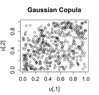
Figure 3.1.: Scatter plot of the Gaussian copula forρ= 0.3

0.0 0.2 0.4 0.6 0.8 1.0

0.

0

0.

4

0.

8 u[,1]

u[

,2]

Gaussian Copula

(19)

0.0 0.2 0.4 0.6 0.8 1.0

0.

0

0.

4

0.

8 u[,1]

u[

,2]

Gaussian Copula

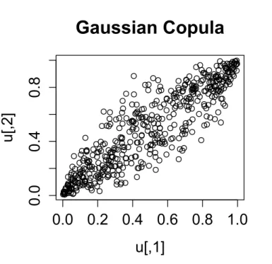
Figure 3.3.: Scatter plot of the Gaussian copula forρ= 0.9

It is interesting to note that Gaussian (Normal) copulas have zero tail dependence (λU = λL = 0). See Embrechts et al. [2003] for a proof of this result. Using R, scatter plots of the bivariate Gaussian copula for various values of the correlation parameter ρ = 0.3 , ρ = 0.6 and ρ= 0.9 are shown in Figures 3.1, 3.2 and 3.3 respectively. The symmetry of the Gaussian copula can also be seen in these scatter plots.

The Gaussian copula plots for ρ= 0.3 andρ= 0.6 (Figures 3.1 and 3.2) show that Gaussian copulas do not have upper tail dependence and lower tail dependence (λU =λL= 0) except in

the special case withρ close to 1 (Figure 3.3), where there is perfect correlation. However, this approach does not show tail dependence.

As mentioned in Economist [2009] and Bogard [2011], the Gaussian copula was used widely before the housing crisis to simulate the dependence between housing prices in various geo-graphic areas. Looking at the scatter plots for the Gaussian copulas above, it can be seen that extreme events (very high values ofU1andU2or very low values ofU1andU2) seem very weakly

correlated. Archimedean copulas, e.g. Clayton and Gumbel copulas are good alternatives to Gaussian copula.

3.6. Archimedean Copulas

(20)

and range [0,∞) satisfying ϕ(0) = ∞ and ϕ(1) = 0. Use ϕ−1 _{for the inverse function of} _ϕ_.

Then Archimedean copulas are defined as;

Cϕ(u1, u2) =ϕ−1(ϕ(u1) +ϕ(u2)) u1, u2 ∈(0,1]

whereϕis called a generator function of te CopulaCϕ. The Archimedean representation allows

us to reduce the study of a multivariate copula to a single univariate function. Archimedean copulas have a commutative property, i.e. Cϕ(u1, u2) =Cϕ(u2, u1). This class family of copulas

have many different forms and you can see three often used Archimedean copulas in the following subsections.

3.6.1. Clayton Copula

The Clayton copula is also known as Cook-Johnston copula, whose generator ϕθ is defined by

ϕθ(u) =

1

θ(u

−θ₋₁₎

Hence, the Clayton copula is in the form of:

Cθ(u1, u2) =

u−₁θ+u−₂θ−1−1/θ

The upper tail dependence measure for Clayton copula is zero (λU = 0) and the lower tail

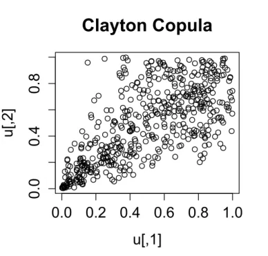
dependence measure is positive (λL= 2−1/θ >0). See Panjer [2006] for a proof of these results. The Clayton copula has a single parameterθthat can be estimated from data using a statistical methods, such as maximum likelihood. UsingR, scatter plots of the bivariate Clayton copula for various values ofθ= 0.5 ,θ= 2 andθ= 10 are shown in Figures 3.4 , 3.5 and 3.6 respectively.

0.0 0.2 0.4 0.6 0.8 1.0

0.

0

0.

4

0.

8 u[,1]

u[

,2]

Clayton Copula

(21)

0.0 0.2 0.4 0.6 0.8 1.0

0.

0

0.

4

0.

8 u[,1]

u[

,2]

Clayton Copula

Figure 3.5.: Scatter plot of the Clayton copula for θ= 2

0.0 0.2 0.4 0.6 0.8 1.0

0.

0

0.

4

0.

8 u[,1]

u[

,2]

Clayton Copula

Figure 3.6.: Scatter plot of the Clayton copula for θ= 10

(22)

Clayton copula 3.4, 3.5 and 3.6 above that the higher the value of θ, the more the two random variables depend on each other in lower tail. As mentioned in B¨urgi et al. [2008], the Clayton copula is not symmetric and acts on the lower tail of the distribution, whereas for upper tail the random variables are hardly dependent on each other. In insurance, however, the dependence should be modeled for the upper tails. This can easily be obtained by mirroring the copula by a transformation (u1, u2)−→(1−u1,1−u2).

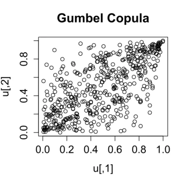
3.6.2. Gumbel Copula

The Gumbel copula is also known as the Gumbel-Hougaard copula and has the generator:

ϕθ(u) = (−lnu)θ θ≥1

Hence, the Gumbel copula has the form:

Cθ(u1, u2) = exp

−h(−lnu1)θ+ (−lnu2)θ

i1/θ

The measure of upper tail dependence isλU = 2−21/θ. See Panjer [2006] for a proof of this

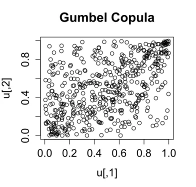
result. The Gumbel copula also has a single parameterθ. UsingR, scatter plots of the bivariate Gumbel copula for various values of θ = 1.5 , θ = 2 and θ = 5 are shown in Figures 3.7 , 3.8 and 3.9 respectively.

0.0 0.2 0.4 0.6 0.8 1.0

0.

0

0.

4

0.

8 u[,1]

u[

,2]

Gumbel Copula

(23)

0.0 0.2 0.4 0.6 0.8 1.0

0.

0

0.

4

0.

8 u[,1]

u[

,2]

Gumbel Copula

Figure 3.8.: Scatter plot of the Gumbel copula for θ= 2

0.0 0.2 0.4 0.6 0.8 1.0

0.

0

0.

4

0.

8 u[,1]

u[

,2]

Gumbel Copula

Figure 3.9.: Scatter plot of the Gumbel copula for θ= 5

(24)

B¨urgi et al. [2008], in comparison to the Clayton copula, the Gumbel dependence acts on both upper and lower tails. Nevertheless, the Gumbel copula is not symmetric, i.e. the dependence of high Quantiles is stronger than the one of low Quantiles.

Simulations using copulas can be implemented in R package copula (see Yan et al. [2007]

”Enjoy the joy of copulas: with a package copula”). The R codes that I have used to create

(25)

4. Copula-based hierarchical model for risk

aggregation

We discuss copula-based hierarchical approach for risk aggregation and dependence modeling here. In the next chapter, to empirically illustrate this method we will apply the hierarchical aggregation model to the real data, Danish fire insurance data, in detail and present some conclusions. This chapter is inspired by the paper on ”Copula based hierarchical risk aggregation through sample reordering” (Arbenz et al. [2012]).

The objective of risk aggregation and dependence modeling is to model adequately dependent insurance portfolios in order to evaluate the overall risk exposure. In risk aggregation we are interested in the distribution of sum of insurance claims:

S=

d X

i=1

Xi

whereXiare the value of losses due to some risks that are correlated. Dependence between risks

cannot be ignored and their dependence must be modelled appropriately. As outlined in the previous chapters, there are three popular risk aggregation methods and modeling dependence structure in insurance:

• variance-covariance method

• risk factor models

• copula models

But each of these three models has its own weaknesses and in high dimensions, they become problematic (see Arbenz [2012]):

- In variance-covariance method, the conclusions that can be drawn from this model are

only limited to the first and second moments, i.e. mean, variance and covariance of the risks X1, . . . , Xd, and thus further properties of the distribution of sum of the risks, S,

cannot be understood. Number of correlation parameters in this method (=d(d−1)/2) become confusingly large in high dimensions.

- Inrisk factor method, modelling risk factors and estimating risk factor sensitivities for all

risks can be difficult in high dimensions.

- In copula models, fitting a copula in high dimensions is problematic. The number of

(26)

Hierarchical risk aggregation model can avoid the above problems. In this method we do not need to specify the whole multivariate dependence structure. It is enough to specify lower dimensional dependence structures for each of the aggregation steps. We can obtain the distri-bution of sum of the risks using partial sums. This method is appropriate for high dimensional problems, but for making it clearer we will consider a simple three-dimensional problem exam-ple.

4.1. Hierarchical aggregation

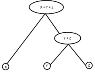
This model consists of an aggregation tree structure, marginal distributions for each risk and bivariate copulas for each aggregation step. Suppose we have three risksX, Y, Z and we want to compute the distribution of sum of these three risks, i.e. the total aggregateS;

S=X+Y +Z

The classical copula approach consists of modelling the joint distribution of (X, Y, Z) using one trivariate copula CX,Y,Z(FX(x), FY(y), FZ(z)) and directly computing the distribution of sum, S. Instead, we do the”hierarchical aggregation approach”, in the following steps;

(1) We set the aggregation tree structure. Number of tree structures to aggregate 3 risks is equal to 3, to aggregate 4 risks is equal to 15 and so on. To set the aggregation tree structure, first we select the greatest dependencies either positive or negative, i.e. we select the two risks Xi, Xj that are most dependent (based on Kendall’s tau τ) and combine

them. The aggregation tree structure of this example is shown in Figure (4.1). In this specific case, a joint model for the pair (X, Y) would first be constructed. For further details on existence and uniqueness of aggregation tree structure we refer to Arbenz et al. [2012].

(27)

(2) We have to specify the marginal distributions for each three risks X,Y, Z and estimate their parameters:

FX(x) =P[X≤x] FY(y) =P[Y ≤y] FZ(z) =P[Z≤z].

(3) We model the dependence structure among X and Y with a bivariate copula CX,Y: P[X≤x, Y ≤y] =CX,Y(FX(x), FY(y)).

This determines the distribution of the bivariate random vector (X, Y), and as a result, it determines the distribution of the sub-aggregateT:

T =X+Y.

The cumulative distribution function (FT) of sub-aggregateT is given by:

FT(t) =P[X+Y ≤t] = Z

R2✶

{x+y≤t} dCX,Y(FX(x), FY(y)).

where✶{x+y≤t} is an indicator function defined as:

✶{x+y≤t}=

1 ifx+y≤t

0 ifx+yt

(4) Having fixed the distribution of T =X+Y in the previous step, we would build a joint model for the pair (T, Z) by combining FT and FZ using the bivariate copula CT,Z:

P[T ≤t, Z ≤z] =CT,Z(FT(t), FZ(z)).

This determines the distribution of the bivariate random vector (T, Z), and as a result, it determines the distribution of the total aggregate S:

S=T +Z =X+Y +Z.

The cumulative distribution functionFS of total aggregate S is given by:

FS(s) =P[T +Z ≤s] = Z

R2✶

{t+z≤s} dCT,Z(FT(t), FZ(z)).

This approach has many advantages. As mentioned above, in the classical copula approach for the calculation of the distribution of the sum of three risks,S =X+Y +Z, we would determine the trivariate copulaCX,Y,Z. As opposed to the classical approach, the hierarchical aggregation

model involves only two bivariate copulas CX,Y and CT,Z. This is an advantage when the

number of risks is large, i.e. in higher dimensions. In general, the hierarchical aggregation for d risks (X1, X2, . . . , Xd) can be modelled as follows. First, select and combine the two

risks (Xi, Xj) that are most dependent through a bivariate copula model CXi,Xj. Kendall’s

tau dependence measure can used to determine the order in which risks are aggregated. Next, replace the individual risks Xi and Xj by their sum Sij =Xi+Xj and repeat these steps for

the new combined risk and the remaining risks, i.e. it leaves one new aggregation tree with

d−1 risks, that the procedure can be repeated for the new tree. Continue this procedure in a iterative way until all the risks have been aggregated in a single sum S=X1+. . .+Xd. This

(28)

4.2. Reordering algorithm for the numerical approximation

After the above steps in the hierarchical aggregation approach, i.e. selecting the aggregation tree structure, finding the marginal distributions for each risk, and fitting the bivariate copulas for each aggregation step, we need to numerically approximate the hierarchical risk aggregation structure. The ”reordering algorithm” allows us to do it. Classical multivariate models use approximations through i.i.d. sampling (Monte Carlo simulations), but generating i.i.d. samples from this aggregation tree is not possible because it is not easy to deal numerically with the joint density (if existing) of all risks (X, Y, Z) and the copula function between all risksCX,Y,Z. Instead of the classical i.i.d. sampling, we suggest the reordering algorithm for approximation that is inspired by the the Iman-Conover method (see Arbenz et al. [2012]). In this section we discuss the reordering algorithm that obtains numerical approximations through a bottom-up approach. For illustrative purposes, we again suppose we have three risks X, Y, Z example as described in the previous section. Therefore, our purpose is to approximate the distribution function of total aggregate:

S=T+Z = (X+Y) +Z.

Assume the marginal distributions ofX, Y, Z are estimated and given by:

FX(x) =P[X ≤x] FY(y) =P[Y ≤y] FZ(z) =P[Z ≤z].

And two bivariate copulas CX,Y and CT,Z are fitted and given by;

P[X ≤x, Y ≤y] =CX,Y(FX(x), FY(y))

P[T ≤t, Z ≤z] =CT,Z(FT(t), FZ(z)).

We do the reordering algorithm using the following steps;

(1) Fix numbern.

(2) Simulate independently marginal samples of size nfromX,Y and Z; - Xi ∼FX

- Yi ∼FY

- Zi ∼FZ

fori= 1, . . . , n.

(3) Simulate independently copula samples of sizenfrom CX,Y and CT,Z; - Ui ∼CX,Y

- Vi ∼CT,Z

fori= 1, . . . , n.

(4) For the first aggregation step, construct the bivariate reordered samples of (X, Y) by reordering the marginal samplesXi and Yi based on the joint ranks of the copula sample Ui. Thus we get a sample of T by summing upT =X+Y.

(29)

(6) Define the empirical distribution function forS.

Thanks to Dr. Philipp Arbenz for putting the reordering algorithm R code program in his web pagehttps://sites.google.com/site/philipparbenz/. For illustrating hierarchical aggregation through reordering algorithm, we give a trivariate example here:

We choose equal marginal distributions for all three risks. As mentioned in (B¨urgi et al. [2008]), the biggest effect of dependence can be seen when aggregatingequal risks. A canonical type of aggregate loss model used in insurance is the lognormal distribution. Therefore, we choose lognormal marginal distributions with parameters meanlog µ = 1 and sdlog σ = 1 for each risk in our example. For generating the copula samples, we use Clayton copulas that is the most asymmetric one of the copulas (Clayton copula with parameterθ= 2 for first aggregation step and with parameter θ = 1 for second aggregation step). Recall that the Clayton copula is in the form of Cθ(u1, u2) =

u−₁θ+u−₂θ−1−1/θ. We do the reordering algorithm example using the following steps:

• Fix number of simulations n= 4.

• Generate lognormal marginal samples i.i.d. Xi ∼ Lognormal(µ = 1, σ = 1), for i =

1,2,3,4, and then sort them. We denote the sorted Xi with notation X(i). This gives:

X(1) = 0.56 X(2)= 0.64 X(3)= 1.60 X(4) = 5.83

• Generate lognormal marginal samples i.i.d. Yi ∼Lognormal(µ= 1, σ = 1), independent

of the Xi. Then sort them. We denote the sorted Yi with notation Y(i). This gives:

Y₍₁₎ = 0.67 Y₍₂₎= 2.40 Y₍₃₎= 4.53 Y₍₄₎= 19.37

• Generate Clayton copula i.i.d. samples Ui= (Ui1, Ui2), independent of the Xi and Yi. the

copula simulation yielded the following samples:

(U₁1, U₁2) = (0.74,0.54) (U₂1, U₂2) = (0.46,0.92)

(U₃1, U₃2) = (0.92,0.70) (U₄1, U₄2) = (0.35,0.38)

• Obtain the joint ranks of the copula samples. We denote the joint ranks with notation (R1_i, R2_i). This gives:

(R1₁, R2₁) = (3,2) (R1₂, R2₂) = (2,4) (R1₃, R2₃) = (4,3) (R1₄, R2₄) = (1,1)

• Reorder and couple the samplesX₍_i₎ and Y₍_i₎such that the new bivariate sample has the same joint ranks as the copula samples. This gives the bivariate sample (X₍_R1

i), Y(R

2

i)) of:

(X₍_R1 1), Y(R

2

1)) = (X(3), Y(2)) = (1.60,2.40) (X(R 1 2), Y(R

2

2)) = (X(2), Y(4)) = (0.64,19.37)

(X₍_R1 3), Y(R

2

3)) = (X(4), Y(3)) = (5.83,4.53) (X(R 1 4), Y(R

2

4)) = (X(1), Y(1)) = (0.56,0.67)

• Calculate samples of the sub-aggregateT =X+Y by taking the component wise sum of the bivariate reordered samples (X₍_R1

i), Y(R

2

i)) above. This gives:

T1=X(3)+Y(2) = 1.60 + 2.40 = 4.00 T2=X(2)+Y(4)= 0.64 + 19.37 = 20.01

(30)

• Repeat the previous procedure for samples Ti and Zi ∼ Lognormal(µ = 1, σ = 1) and

reorder the samplesTi and Zi such that their linked ranks are equal to the joint ranks of

the copula samplesV = (V_i1, V_i2). This gives the following results: Sorted sub-aggregate samples T₍_i₎:

T₍₁₎ = 1.23 T₍₂₎ = 4.00 T₍₃₎= 10.36 T₍₄₎ = 20.01

Sorted lognormal marginal samplesZ(i):

Z₍₁₎= 1.15 Z₍₂₎= 1.53 Z₍₃₎ = 2.01 Z₍₄₎ = 21.97

Clayton copula simulationV = (V1

i , Vi2) yielded:

(V₁1, V₁2) = (0.02,0.28) (V₂1, V₂2) = (0.34,0.06)

(V₃1, V₃2) = (0.33,0.40) (V₄1, V₄2) = (0.17,0.09) Joint ranks of the copula samples:

(R1₁, R2₁) = (1,3) (R1₂, R2₂) = (4,1)

(R1₃, R2₃) = (3,4) (R1₄, R2₄) = (2,2) Reordered bivariate sample (T₍_R1

i), Z(R

2

i)) according to the joint ranks of the copula V

samples:

(T₍_R1 1), Z(R

2

1)) = (T(1), Z(3)) = (1.23,2.01) (T(R 1 2), Z(R

2

2)) = (T(4), Z(1)) = (20.01,1.15)

(T₍_R1 3), Z(R

2

3)) = (T(3), Z(4)) = (10.36,21.97) (T(R 1 4), Z(R

2

4)) = (T(2), Z(2)) = (4.00,1.53)

• Calculate samples of the total aggregateS =T+Z =X+Y +Z by taking the component wise sum of the bivariate reordered samples (T₍_R1

i), Z(R

2

i)) above. This gives:

S1=T(1)+Z(3) = 1.23 + 2.01 = 3.24 S2 =T(4)+Z(1)= 20.01 + 1.15 = 21.16

S3=T(3)+Z(4) = 10.36 + 21.97 = 32.33 S4=T(2)+Z(2) = 4.00 + 1.53 = 5.53

This defines the empirical distribution function for the total aggregateS as:

F_Sn(s) =F_S4(s) = 1

4✶{3.24≤s}+ 1

4✶{21.16≤s}+ 1

4✶{32.33≤s}+ 1

4✶{5.53≤s} where✶{.}is an indicator function.

The reordering algorithm produces the approximations of the distributions of (X, Y), (T, Z), and S. The final result, F_S4, is an empirical distribution function for the total aggregate S. Suppose the FS is the cumulative distribution function of S, then F_S4 is an approximation

of FS. In general, for fixed number of simulations n, the FSn is an approximation of FS. A

theorem given in (Arbenz et al. [2012], subsection 3.2, page 7) proves that when n→ ∞, we obtain convergenceFn

S →FS.

(31)

5. Application to Danish Fire Insurance Data

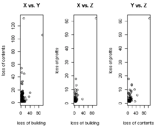
These Danish Fire Insurance Data were collected at Copenhagen Reinsurance and comprise 2167 fire losses over the period 1980 to 1990 and are expressed in millions of Danish Krone (DKK). Every total claim has been divided into three risks consisting of a building loss, a loss of contents and a loss of profits caused by the same fire. These three risks in our study are denoted by:

X = loss of building Y = loss of content Z = loss of profit

As mentioned in Esmaeili and Kl¨uppelberg [2010], Haug et al. [2011] and Dreesa and M¨ullerb [2007], the claims are recorded only if the sum of all three risks is greater or equal to 1 million Danish Kroner (DKK). Because of this, there is an artificial negative dependence between the risks components X, Y and Z, i.e. if one risk component is smaller than 1 million DKK, the sum of the others must be accordingly larger. Therefore,we assume the values in each risk component had been truncated from below at 1 million DKK. The risksX ,Y and Z

are clearly dependent, as can be seen from Figure 5.1. Note that the number of observations is not the same each time I consider a pair of risks.

(32)

5.1. R Packages fitdistrplus and copula

Here we briefly introduce two important R packages. In the following subsections we are frequently using these R packages to statistically analyze this data set. The copula package provides a platform for multivariate modeling with copulas inR (see Yan et al. [2007] and Ko-jadinovic et al. [2010]). We are usingcopula package for constructing Archimedean copula and Elliptical copula class objects with its corresponding parameters and dimension, goodness-of-fit tests and parametric estimation for copulas, and multivariate independence test of continuous random variables based on the empirical copula process.

In fitdistrplus package, the multivariate Danish Fire Insurance Data set is stored in

”dan-ishmulti”. This data set has been divided into a building loss, a loss of contents and a loss of profits (see Delignette-Muller and Dutang [2014]). In this package,”danishmulti” contains five columns:

- Date: The day of claim occurence.

- Building: The loss amount (mDKK) of the building coverage.

- Contents: The loss amount (mDKK) of the contents coverage.

- Profits: The loss amount (mDKK) of the profit coverage.

- Total: The total loss amount (mDKK).

where all columns are numeric except Date columns of class Date. We can import the multi-variate Danish Fire Insurance Data set inR by:

> library(fitdistrplus) > data(danishmulti)

5.2. Determination of the tree structure, hierarchical clustering

As mentioned in section 4.1 in the previous chapter, to determine the aggregation tree structure, first we select the two risks that are most dependent and combine them. Kendall’s tau depen-dence measure can be used to determine the order in which risks are aggregated. A procedure for selecting the tree structure based on Kendalls tau τ is called ”hierarchical clustering

tech-nique”. Consider two arbitrary risks Xi and Xj. The measure of distanceD(Xi, Xj) between

these two risks based on Kendall’s tauτ is defined as:

D(Xi, Xj) = q

1−τ2₍_X

i, Xj) (5.1)

where τ(Xi, Xj) denotes Kendall’s tau dependence measure between pair Xi and Xj. The principle of hierarchical clustering method is to identify the two risks that are the closest, i.e. the measure of distanceD is minimal for them, and then to combine them into a group. Then we repeat this procedure until only one risk is left (see Cˆot´e and Genest [2015]). As can be seen from equation (5.1), the minimal measure of distanceD is related to the largest Kendall’s tauτ dependence measure. Therefore, first we select and model the two risks with the largest Kendall’s tauτ.

(33)

> cor.test(contents, profits, method = "kendall", alternative = "greater")

We foundp-values of 2.495e−08 for (X, Y), 0.001346 for (X, Z) and 4.629e−06 for (Y, Z) that they are all less than 0.05 significance level. Hence we reject the null hypothesis and Kendall’s tauτ is significantly greater than zero. It can be seen this result from Figure 5.1 also, that the risks are clearly dependent. Recall that X = loss of building, Y = loss of content, Z = loss of profit.

We apply the function ”cor” with the ”kendall” option inRfor comparison of Kendall’s tau

τ between three different pairs of components of danish fire insurance data. For instance:

> cor(contents, profits, method="kendall")

After applying function ”cor”, we got these results:

τ(X, Y) = 0.211032, τ(X, Z) = 0.261722, τ(Y, Z) = 0.328090

From equation (5.1) we could calculate the measure of distanceD:

D(X, Y) = 0.977480, D(X, Z) = 0.965143, D(Y, Z) = 0.944646

The measure of distance D(Y, Z) is the smallest one, i.e. Y and Z are the closest. Thus we first construct the joint model for the pair (Y =”loss of contents” , Z =”loss of profits”). The aggregation tree structure of this data set is shown in Figure 5.2.

Figure 5.2.: An aggregation tree structure of Danish Fire Insurance Data.

5.3. Choice of marginal distributions for the risks

We have to specify the marginal distributions for theX= loss of building,Y = loss of contents,

(34)

Histogram of loss of building

Building

Densit

y

0 50 100 150

0. 0 0. 1 0. 2 0. 3 0. 4 0. 5

Histogram of loss of contents

Contents

Densit

y

0 20 40 60 80 100 120

0. 0 0. 1 0. 2 0. 3 0. 4

Histogram of loss of profits

Profits

Densit

y

0 10 20 30 40 50 60

0. 0 0. 1 0. 2 0. 3 0. 4 0. 5

(35)

The most direct way to see how well a distribution fits a data set is to plot the respective histogram, which can suggest a kind of distribution to use to fit the model. These plots are a very useful guide to heavy-tailedness. We present the histogram of each risk X, Y and

Z in Figure 5.3. A first glance at Figure 5.3 clearly shows heavytailedness and skewness to the right for each data set. The danish fire insurance data show Pareto tail behaviour. The

Single-parameter Pareto distribution is a classical skewed, heavy-tailed distribution. We estimate parameter shape (α) of Single-parameter Pareto distribution fitted to loss of building by maximum likelihood estimation method.

The Single-parameter Pareto distribution with parameter shape = α has PDF and CDF:

f(x) = αθ

α

xα+1 x > θ.

F(x) = 1−

θ x

α

x > θ.

Although there appears to be two parameters, only parameter shape = α is a true parameter. The value of lower bound = θ must be set in advance. In our caseθ= 1.

The Maximum Likelihood Estimation method (MLE) is the most popular method to estimate the distribution parameters from an empirical sample. It finds the model parameters that maximize the likelihood of the observed data with respect to the theoretical model. One of the attractive properties of the Single-parameter Pareto distribution is the ease of calculation of the maximum likelihood estimate of the parameter.

In general, the likelihood function for Single-parameter Pareto distribution with parameter shape =α, given datatruncatedfrom below atθ, is:

L(α) =

n Y

j=1

f(xj |α)

1−F(θ|α)

Note that in Single-parameter Pareto distribution the lower bound is equal to truncation point (θ = 1) and the Survival function at lower bound (1−F(θ|α)) = 1. Therefore the likelihood function is:

L(α) =

n Y

j=1

α xα_j+1

The logarithmic likelihood function is:

l(α) =

n X

j=1

(lnα−(α+ 1)ln(xj))

=nlnα−(α+ 1)

n X

j=1

ln(xj)

To find the estimator for α, we compute the corresponding partial derivative and determine where it is zero:

∂l ∂α = n α − n X j=1

ln(xj) = 0

Thus the maximum likelihood estimator forα is: ˆ

α= _Pn n

(36)

As a result of above formula, we got parameter shape estimationα= 1.587 and lower bound

θ= 1 for loss of building.

These real data are surely not exactly Single-parameter Pareto distributed, and for most practical applications the question would be ”how good is the Single-parameter Pareto approx-imation?”. The Q-Q plot is a good way to show the quality of such an approximation. A Q-Q plot represents the quantiles of the theoretical fitted distribution against the empirical quantiles of the data. The Q-Q plot of loss of building data against its estimated Single-parameter Pareto distribution is shown in Figure 5.4.

Figure 5.4.: Q-Q plot of loss of building data against its estimated Single-parameter Pareto distribution.

Any way we can do our test with the Kolmogorov-Smirnov statistic, after estimating the parameters by maximum likelihood. The KolmogorovSmirnov statistic quantifies a distance be-tween the empirical distribution function of the sample and the cumulative distribution function of the reference distribution. We perform K-S test using ks.test function inR:

> ks.test(Building, "ppareto1", shape = 1.587, min = 1)

We got the following Routput:

################################################### One-sample Kolmogorov-Smirnov test

data: Building

D = 0.0699, p-value = 1.324e-06 alternative hypothesis: two-sided

###################################################

(37)

Many articles have used the same danish fire insurance data and concluded that this data follows different distributions (see Esmaeili and Kl¨uppelberg [2010], Haug et al. [2011], Dreesa and M¨ullerb [2007] and McNeil [1997]). Although these data are surely not exactly Single-parameter Pareto distributed, I assume they follow Single-Single-parameter Pareto distribution in this thesis for the purposes of illustration of the hierarchical aggregation model.

Therefore, we select a marginal distribution Single-parameter Pareto for loss of building with parameter shape α = 1.587 and lower bound θ = 1. In a similar way, we select the marginal Single-parameter Pareto distribution for loss of contents with parameter shape α= 1.085 and loss of profits with parameter shapeα= 1.038.

5.4. Choice of bivariate copulas

After determination of the aggregation tree structure, we select an appropriate bivariate copula at each aggregation step. I am analyzing the dependence only in the tails. As explained above, we first construct the joint model for the pair (Y =”loss of contents” , Z =”loss of profits”) at first aggregation step because they are the two risks that are most dependent. To check the null hypothesis of independence of loss of contents and loss of profits, we implement an independence test using functionsindepTestSim andindepTestof thecopulapackage inR. This independence test consists of two steps: (i) indepTestSim function: a simulation step, which consists of simulating the distribution of the test statistics under independence for the sample size under consideration; (ii)indepTestfunction: the test itself, which consists of computing the approximate p-values of the test statistics with respect to the empirical distributions obtained in the first step (see Kojadinovic et al. [2010]). We apply the independence test to loss of contents and loss of profits:

> cp <- cbind(contents , profits)

> empsamp <- indepTestSim(nrow(cp), p = 2, N=1000) > indepTest(cp,empsamp)

We obtain theR output:

######################################################################## Global Cramer-von Mises statistic: 0.2200595 with p-value 0.0004995005 Combined p-values from the Mobius decomposition:

0.0004995005 from Fisher’s rule, 0.0004995005 from Tippett’s rule.

########################################################################

These p-values give strong evidence against the null hypothesis of independence at the 0.05 significance level. The independence is rejected, and the next step is to fit an appropriate parametric copula CY,Z function to the pair (Y =”loss of contents” , Z =”loss of profits”).

As candidate copulas, we consider Gaussian (Normal), Clayton and Gumbel copula families to model the dependence among Y and Z. We perform several goodness-of-fit tests for these copula families usinggofCopula function incopula package:

> normal.cop <- normalCopula(0.6, dim=2) > gofCopula(normal.cop, cp)

(38)

> gofCopula(clayton.cop, cp)

> gumbel.cop <- gumbelCopula(2, dim=2) > gofCopula(gumbel.cop, cp)

We found approximatep-values of 0.004496 for Normal copula, 0.0004995 for Clayton copula and 0.1683 for Gumbel copula respectively. Therefore, among all candidate copula families that we have tested, the Gumbel copula is the only one that is not rejected at the 0.05 significance level because itsp-value is greater than 0.05. The parameter estimate for the copula fit is computed by the pseudo maximum likelihood method. ThegofCopula function also returns the estimate of the parameters of the Gumbel copula, θ= 1.534. In a similar way, we select an appropriate bivariate parametric copula CX,T, Gumbel copula with parameter estimate θ= 1.282, for the

pair (X, T) at the second aggregation step where

X = loss of building T = (Y +Z) = (loss of contents + loss of profits)

5.5. Hierarchical aggregation through reordering algorithm

After determining the aggregation tree structure, finding the marginal distributions for each risk, and fitting the bivariate copulas for each aggregation step, we need to numerically approximate the hierarchical risk aggregation structure. We do it through reordering algorithm. As explained in the previous chapter, we do the reordering algorithm using the following steps:

(1) Fix number of simulations n= 1000.

(2) Generate Single-parameter Pareto marginal i.i.d. samples of sizen= 1000 fromX,Y and

Z;

- Xi ∼Single-parameter Pareto(α= 1.587)

- Yi ∼Single-parameter Pareto(α= 1.085)

- Zi ∼Single-parameter Pareto(α= 1.038)

fori= 1, . . . ,1000.

(3) Generate copula i.i.d. samples of sizen= 1000 fromCY,Z, Gumbel copula with parameter θ= 1.534, andCX,T, Gumbel copula with parameterθ= 1.282;

- Ui ∼CY,Z

- Vi ∼CX,T

fori= 1, . . . ,1000.

(4) For the first aggregation step, construct the bivariate reordered samples of (Y, Z) by reordering the marginal samples Yi and Zi based on the joint ranks of the copula sample Ui. Thus we get a sample of T by summing upT =Y +Z.

(39)

(6) Calculate the samples of the total aggregate S. Denote by S1, . . . , S1000 the simulated

samples of S. The empirical distribution function forS is defined as:

F_Sn(s) =F_S1000(s) = 1 1000

1000

X

i=1

✶{Si ≤s}

where✶{.}is an indicator function.

5.6. Conclusions and results

Suppose thatFSis the cumulative distribution function ofS, thenFS1000is a good approximation

of FS. R provides a very useful function ecdf for working with the empirical distribution

function. It computes or plots an empirical cumulative distribution function. Theecdf function applied to a data sample returns a function representing the empirical cumulative distribution function. Let’s use the ecdf() function to obtain some empirical CDF values ofS. For example it is possible to see what the output looks like below:

> Fn <- ecdf(S) > Fn(3.04) [1] 0.001 > Fn(40) [1] 0.943 > Fn(100) [1] 0.976

The empirical cumulative distribution function of S is shown in Figure 5.5.

(40)

We present the histogram plot of the total aggregate samples S in Figure 5.6 to examine the distribution of S.

Figure 5.6.: Histogram and Density estimate of the total aggregate S

As can be seen in this master thesis, the copula-based hierarchical aggregation model through

reordering algorithm provides a simple and practical framework to model the distribution of the

(41)

A. Appendix A

The R codes that I used to create the scatter plots of the bivariate Gaussian, Clayton and Gumbel copulas:

> library("copula") > set.seed(1)

# Gaussian Copula

> norm.cop <- normalCopula(0.3) > norm.cop

> u <- rcopula(norm.cop, 500) > plot(u)

> title("Gaussian Copula")

# Clayton Copula

> clayton.cop <- claytonCopula(0.5) > clayton.cop

> u <- rcopula(clayton.cop,500) > plot(u)

> title("Clayton Copula")

# Gumbel Copula

> gumbel.cop <- gumbelCopula(1.5) > gumbel.cop

> u <- rcopula(gumbel.cop,500) > plot(u)

(42)

B. Appendix B

The R programming code that used for the implementation of the reordering algorithm for the mentioned trivariate example:

# load package ’copula’ library > library(copula)

# fix number of simulations > n

# generate marginal samples. Here, lognormal distributions is used. > X = rlnorm(n, 1, 1)

> Y = rlnorm(n, 1, 1) > Z = rlnorm(n, 1, 1)

# generate copula samples. Here, Clayton copulas is used. > U = rcopula(claytonCopula(param = 2, dim = 2), n)

> V = rcopula(claytonCopula(param = 1, dim = 2), n)

# reordering according to U > X[order(U[,1])] = sort(X) > Y[order(U[,2])] = sort(Y) > print(cbind(X,Y) , digits=3)

# calculate samples of the sub-aggregate T > T = X+Y

# reordering according to copula V > T[order(V[,1])] = sort(T)

> Z[order(V[,2])] = sort(Z) > print(cbind(T,Z) , digits=3)

# calculate total aggregate S > S = T+Z

# final result

(43)

List of Figures

3.1. Gaussian Copula forρ= 0.3 . . . 13

3.4. Clayton Copula forθ= 0.5 . . . 15

3.5. Clayton Copula forθ= 2 . . . 16

3.6. Clayton Copula forθ= 10 . . . 16

3.7. Gumbel Copula forθ= 1.5 . . . 17

3.8. Gumbel Copula forθ= 2 . . . 18

3.9. Gumbel Copula forθ= 5 . . . 18

4.1. An aggregation tree structure involving three risks . . . 21

5.1. Bivariate scatterplots of Danish Fire Insurance Data . . . 26

5.2. An aggregation tree structure of Danish Fire Insurance Data . . . 28

5.3. Histograms of loss of building, loss of contents and loss of profits . . . 29

5.4. Q-Q plot of loss of building data against its estimated Single-parameter Pareto distribution . . . 31

5.5. The empirical cumulative distribution function ofS . . . 34

(44)

Bibliography

P. Arbenz. Multivariate Modelling in Non-Life Insurance. PhD thesis, ETH ZURICH, 2012.

P. Arbenz, C. Hummel, and G. Mainik. Copula based hierarchical risk aggregation through sample reordering. Insurance: Mathematics and Economics, 51(1):122–133, 2012.

M. Bogard. Copula functions, r, and the financial crisis. R-bloggers.com, March 2011. URL

http://www.r-bloggers.com/copula-functions-r-and-the-financial-crisis/.

R. B¨urgi, M. M. Dacorogna, and R. Iles. Risk aggregation, dependence structure and diversifi-cation benefit. Stress Testing for Financial Institutions, 2008.

M.-P. Cˆot´e and C. Genest. A copula-based risk aggregation model. Canadian Journal of Statistics, 43(1):60–81, 2015.

M. L. Delignette-Muller and C. Dutang. fitdistrplus: An r package for fitting distributions. 2014.

M. Denuit, J. Dhaene, M. Goovaerts, and R. Kaas. Actuarial Theory for Dependent Risks: Measures, Orders and Models. John Wiley & Sons, 2006.

H. Dreesa and P. M¨ullerb. Modeling dependencies in large claims. 2007.

T. Economist. In defense of the gaussian copula. The Economist online, Apr 2009. URL

http://www.economist.com/blogs/freeexchange/2009/04/in_defense_of_copula.

P. Embrechts, F. Lindskog, and A. McNeil. Modelling dependence with copulas and applications to risk management. Handbook of heavy tailed distributions in finance, 8(1):329–384, 2003.

H. Esmaeili and C. Kl¨uppelberg. Parameter estimation of a bivariate compound poisson process. Insurance: Mathematics and Economics, 47(2):224–233, 2010.

E. W. Frees and E. A. Valdez. Understanding relationships using copulas. North American actuarial journal, 2(1):1–25, 1998.

S. Haug, C. Kl¨uppelberg, and L. Peng. Statistical models and methods for dependence in insurance data. Journal of the Korean Statistical Society, 40(2):125–139, 2011.

I. Kojadinovic, J. Yan, et al. Modeling multivariate distributions with continuous margins using the copula r package. Journal of Statistical Software, 34(9):1–20, 2010.

A. J. McNeil. Estimating the tails of loss severity distributions using extreme value theory. Astin Bulletin, 27(01):117–137, 1997.

A. J. McNeil, R. Frey, and P. Embrechts. Quantitative risk management: concepts, techniques, and tools. Princeton university press, 2010.

(45)

H. H. Panjer. Operational risk: modeling analytics, volume 620. John Wiley & Sons, 2006.

J. Skoglund. Risk aggregation and economic capital. Available at SSRN 2070695, 2010.

J. Yan et al. Enjoy the joy of copulas: with a package copula. Journal of Statistical Software, 21(4):1–21, 2007.