Experiments With The Lucas Asset Pricing Model
Elena Asparouhova
∗Peter Bossaerts
†Nilanjan Roy
‡William Zame
§July 11, 2012
Abstract
For over thirty years, the model of Lucas (1978) has been the platform of research on dynamic asset pricing and business cycles. This model restricts the intertemporal behavior of asset prices and ties those restrictions to cross-sectional behavior (the “eq-uity premium”). The intertemporal restrictions reject the strictest interpretation of the Efficient Markets Hypothesis, namely, that prices should follow a martingale. Instead, prices move with economic fundamentals, and to the extent that these fundamentals are predictable, prices should be too. The Lucas model also prescribes the investment choices that facilitate smoothing of consumption over time and across different types of investors. Here, we report results from experiments designed to test the primitives of the model. Our design overcomes, in novel ways, challenges to generate demand for consumption smoothing in the lab, and to induce stationarity in spite of the finite duration of lab experiments. The experimental results confirm the theoretical price predictions across assets with different risk characteristics, but prices are much more volatile, reacting less to fundamentals than predicted. Investment choices are, in turn, consistent with the excessive volatility. Nevertheless, consumption smoothing (over time and across investor types) largely obtains as predicted.1
∗University of Utah †Caltech
‡Caltech §UCLA
1Financial support from Inquire Europe, the Hacker Chair at the California Institute of Technology
1
Motivation
Over the last thirty years, the Lucas model (Lucas, 1978) has been the main platform that has guided the empirical research on dynamic asset pricing and business cycles. It has also become the dominant source of inspiration to financial regulators and central bankers for policy formulation.
The Lucas model delivers the core cross-sectional prediction of virtually all static asset pricing models, namely that a stock’s expected return increases in the covariation (“beta”) of this return with aggregate consumption. Importantly, however, the Lucas model also provides an extension to the static approach, in making clear predictions about the intertemporal behavior of asset prices, and linking those to the cross-sectional restrictions. Specifically, it predicts that prices should co-move with economic funda-mentals (aggregate consumption), and the amount of co-movement should increase with risk aversion. As such, if cross-sectional dispersion in expected returns is high because risk aversion is high, then the time-series co-movement between prices and eco-nomic fundamentals should be high as well. An immediate consequence is that prices will become predictable from the moment economic fundamentals are predictable.
The latter insight is what makes the Lucas model an invaluable formal framework within which to gauge the true empirical content of the Efficient Markets Hypothesis (EMH; Fama (1991)). Contrary to early versions of the EMH, prices need not follow a random walk (Malkiel, 1999) or even form a martingale (Samuelson, 1973) from the mo-ment agents are risk averse, i.e., exhibit preferences with diminishing marginal utility. As Lucas criticizes in Section 8 of his article (Lucas, 1978): “Within this framework, it is clear that the presence of a diminishing marginal rate of substitution [...] is inconsis-tent with the [martingale] property.” In other words, the Lucas model demonstrated for the first time that return predictability can be consistent with equilibrium.
The Lucas model is the equilibruim outcome from exchange between investors who solve complex dynamic programming problems whereby consumption is smoothed as much as possible given available securities, income flows, knowledge of the nature of dividend and income processes, and prices. The Lucas model leaves out many details; it merely assumes that investors somehow manage to use available markets to trade to Pareto-optimal allocations, and then exploits the resulting existence of a representative agent (an equilibrium construction) to price securities. In a realistic setting – and in gratefully acknowledged. The paper benefited from discussions during presentations at various academic institutions and conferences. Comments from Hanno Lustig, Stijn van Nieuwerburgh, Richard Roll, Ramon Marimon, John Duffy, Shyam Sunder, Robert Bloomfield, and Jason Shachat were particularly helpful.
the experiment that we report on here – there exist fewer securities than states. For Pareto optimality to have any reasonable chance to emerge, markets then have to be dynamically complete (Duffie and Huang, 1985), and investors have to resort to complex investment policies that exhibit the hedging feature at the core of the modern theory of derivatives analysis (Black and Scholes, 1973; Merton, 1973a) and first identified to be relevant for dynamic asset pricing in Merton (1973b). Emergence of the Lucas equilibrium then also requires investors to have correct anticipation of (equilibrium) price processes. The latter makes the Lucas model an instantiation of Radner’s perfect foresight equilibrium (Radner, 1972).
On the empirical side, tests of the Lucas model have invariably been applied to historical price (and consumption) series in the field. Little attention has been paid to its choice (investment) predictions. Starting with Mehra and Prescott (1985), the fit has generally been considered to be poor. Attempts to “fix” the model have concen-trated on the auxiliary assumptions rather than on its primitives. Some authors have altered the original preference specification (time-separable expected utility) to allow for, among others, time-nonseparable utility (Epstein and Zin, 1991), loss aversion (Barberis et al., 2001), or utility functions that assign an explicit role to an important component of human behavior, namely, emotions (such as disappointment; Routledge and Zin (2011)). Others have looked at measurement problems, extending the scope of aggregate consumption series in the early empirical analysis (Hansen and Singleton, 1983), to include nondurable goods (Dunn and Singleton, 1986), or acknowledging the dual role of certain goods as providing consumption as well as collateral services (Lustig and Nieuwerburgh, 2005). Included in this category of “fixes” should be the long-run risks model of (Bansal and Yaron, 2004) because it is based on difficulty in recovering an alleged low-frequency component in consumption (growth).
Evidently, this body of empirical and theoretical research does not question the primitives of the model, namely, the claim that markets settle on a stationary Radner equilibrium where prices are measurable functions of fundamentals. Admittedly, the veracity of equilibration would be difficult to test on field data. The problem is that we cannot observe the structural information (aggregate supply, beliefs about dividend processes, etc.) that is crucial to knowing whether markets settle at an equilibrium. (This is related to the Roll critique (Roll, 1977).) By contrast, laboratory experiments provide control over and knowledge of all important variables. Thus, the goal of our study was to bring the Lucas model to the laboratory and to test its primitives.
One of these primitives concerns return predictability, as argued before. Since Keim and Stambaugh (1986), empirical research on the time-series properties of asset
prices has been confirming that returns have a significant predictable component, even if such predictability is elusive at times because it is hard to recover out-of-sample (Bossaerts and Hillion, 1999). Two possible explanations have been advanced for the observed predictability. One is that it is consistent with versions of the Lucas model. In fact, even some of the most puzzling aspects of predictability have been shown to be equilibrium implications of quite simple assumptions about the structure of the economy (Bossaerts and Green, 1989; Berk and Green, 2004; Brav and Heaton, 2002; Li et al., 2009). The second one is that predictability is an aggregate expression of the many cognitive biases that have been demonstrated at the individual level; this is the core thesis of Behavioral Finance (Bondt and Thaler, 1985). Our research, therefore, was in part meant to inform the controversy about predictability of returns in asset markets as it relates to the EMH. Specifically, we wondered whether we could generate return predictability in the laboratory, and if so, whether its nature was consistent with the Lucas model.
The design of such an experiment is challenging. First, there is the fact that
the Lucas model already assumes that somehow markets generate a Pareto optimal allocations. It is not immediately clear what structure would lead to such an outcome in practice, especially when the number of states is large (relative to the number of traded securities). Second, there is the fact that the Lucas model assumes that the world is stationary, and that it continues forever. Finally, the Lucas model assumes that investment demands are driven primarily by the desire to smooth consumption. Here, we present a novel design that squarely addresses these issues. We let subjects trade two different securities, which, given the binary nature of uncertainty in each period, makes markets potentially dynamically complete, and hence, facilitates the emergence of Pareto optimal allocations. The infinite horizon was easy to deal with: as in Camerer and Weigelt (1996), we introduce a stochastic ending time.
The finite experiment duration, however, made stationarity particularly difficult to induce, as beliefs would necessarily change when time approaches the officially
an-nounced termination of the experiment. Likewise, it was difficult to imagine that
participants cared when they received their consumption (earnings) across periods during the course of the experiment, which would potentially have negated the as-sumption of preference for conas-sumption smoothing. We introduced novel features to the standard design of an intertemporal asset pricing experiment to overcome these challenges. Their validity hinges on an important component of the (original) Lucas model, namely, time-separable utility. We made sure that time separability followed naturally from our design, and would only have failed if participants did not have
expected utility preferences.
Our experiment is related to that of Crockett and Duffy (2010). There are at least two major differences, however. First, we did not induce demand for smoothing by means of nonlinearities in take-home pay as a function of period earnings, but induced it as the result of novel experimental design. The predicted pricing patterns are therefore driven solely by the uncertainty of the dividends of (one of) the assets, exactly as in the original Lucas model, unconfounded by nonlinearities. Second, to avoid endgame effects, and hence, to ensure stationarity, we altered the design in a way that was consistent with the theory. The aims of the two studies were different, though. In Crockett and Duffy (2010), the goal was to show that asset price bubbles did not emerge once Lucas-style consumption smoothing was introduced. The goal here was, as mentioned before, to test the primitives of the Lucas model.
The remainder of this paper is organized as follows. Section 2 introduces the Lucas model by means of a stylized example that will form the basis of the experiment. Section 3 details the experimental design. Section 4 presents the results from a series of six experimental sessions. Section 5 provides discussion. The last section concludes.
2
The Lucas Asset Pricing Model
We envisage an environment with minimal complexity yet one that generates a rich set of predictions about prices across time and allocations across types of investors. Perhaps most importantly, the environment is such that trading is necessary in each period. Inspired by Bossaerts and Zame (2006), we wanted to avoid a situation (as in Judd et al. (2003)), where theory predicts that trade will take place only once. When bringing the setting to the laboratory, it would indeed be rather awkward to give subjects the opportunity to trade every period while the theory predicts that they should not!2
Our environment generates the original Lucas model, which is stationary in levels (dividends, and hence, prices). This is in contrast to the models that have informed empirical research of historical field data. Starting with Mehra and Prescott (1985), these are stationary in growth. Level stationarity is easier to implement in the lab-oratory, and thus is preferred for an experiment that already poses many challenges in the absence of growth. While there is no substantive difference between the level and growth versions of the Lucas model (e.g., in both cases, prices move with funda-2Crockett and Duffy (2010) confirm that it is crucial to give subjects a reason to trade every period in
mentals), the reader is cautioned that results are not isomorphic. For instance, when dividend levels are independently and identically distributed (i.i.d.), dividend growth is not (dividend growth is expected to be high when dividends are low, and low when dividends are low).
We consider a stationary, infinite horizon economy in which infinite-lived agents with time-separable expected utility are initially allocated two types of assets: (i) a Tree that pays a stochastic dividend of $1 or $0 every period, each with 50% chance, independent of past outcomes, and (ii) a (consol) Bond that always pays $0.50.
There is an equal number of two types of agents. Type I agents receive income of $15 in even periods (2, 4, 6,...), while those of Type II receive income of $15 in odd periods. As such, total (economy-wide) income is constant over time. Before period 1, Type I agents are endowed with 10 Trees and no Bonds; Type II agents start with 0 Trees and 10 Bonds.
Assets pay dividends dk,t (k ∈ {Tree, Bond}) before period t (t = 1, 2, ...) starts. At
that point, agents also receive their income, yi,t (i = 1, ..., I), as prescribed above. As
dividends and income are fungible, we refer to them as cash, and cash is perishable. In what follows, ci,t denotes the cash available to agent i in period t . Agents have
common time-separable utility for cash:
Ui({ci,t}∞t=1) = E ( ∞ X t=1 βt−1u(ci,t) ) . (1)
Markets open and agents can trade their Trees and Bonds for cash, subject to a stan-dard budget constraint. To determine optimal trades, agents take asset prices pk,t
(k ∈ {Tree, Bond}) as given, and correctly anticipate (`a la Radner (1972)) that future prices are a time-invariant function of the only variable economic fundamental in the economy, namely, the dividend on the Tree dTree,t. In particular they know that prices
are set as follows:
pk,t= βE[
u0(ci,t+1)
u0(c i,t)
(dk,t+1+ pk,t+1)]. (2)
We shall not go into details here, because the derivation of the equilibrium is standard. Instead, here are the main predictions of the resulting (Lucas) equilibrium. For the parametric illustrations, we set β = 5/6, and we assume constant relative risk aversion; if risk aversion equals 1, agents are endowed with logarithmic utility (u(ci,t) = log(ci,t)).
1. Cross-sectional Restrictions: Because the return on the Tree has higher co-variability (or “beta”) with aggregate consumption (which varies only because of the dividend on the Tree), its equilibrium price is lower than that of the Bond,
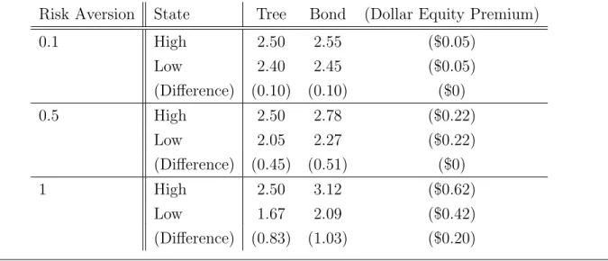
Table 1: Equilibrium Prices And Dollar Equity Premium As A Function Of (Constant Relative) Risk Aversion And State (Level Of Dividend On Tree).
Risk Aversion State Tree Bond (Dollar Equity Premium)
0.1 High 2.50 2.55 ($0.05) Low 2.40 2.45 ($0.05) (Difference) (0.10) (0.10) ($0) 0.5 High 2.50 2.78 ($0.22) Low 2.05 2.27 ($0.22) (Difference) (0.45) (0.51) ($0) 1 High 2.50 3.12 ($0.62) Low 1.67 2.09 ($0.42) (Difference) (0.83) (1.03) ($0.20)
Table 2: Equilibrium Returns And (Percentage) Equity Premium As A Function Of State (Level Of Dividend On Tree), Logarithmic Utility (Risk Aversion = 1).
State Tree Bond (Equity Premium)
High 3.4% -0.5% (3.9%)
replicating a well-known result from static asset pricing theory. Note that this result is far from trivial: returns are determined not only by future dividends, but also future prices, and it is not a priori clear that prices behave like divi-dends! With logarithmic utility, the difference between the price of the Tree and that of the Bond is $0.62 if the dividend on the Tree is high ($1), and $0.42 when this dividend is low ($0). See Table 1. This table also lists prices and cor-responding equity premia for risk aversion coefficients equal to 0.5 (square-root utility) and 0.1.3 We refer to the difference between the Bond and Tree prices as the equity premium. Usually, the equity premium is defined as the difference in expected returns (between a risky benchmark and a relatively riskfree security). To avoid confusion, we refer to our version of the equity premium as the dollar equity premium. For logarithmic preferences, the results translate into expected (percentage) returns and percentage equity premia as in Table 2.
2. Intertemporal Restrictions: Asset prices depend on the dividend of the Tree. As such, prices depend on fundamentals, a key prediction of the Lucas model. The explanation is that when dividends are abundant (the state is High), agents need to be incentivized to consume the (perishable) dividend rather than buying assets. Markets provide the right incentives by pricing the assets dearly. Con-versely, in the Low state, agents should be induced to save and invest rather than consume, which is accomplished through low pricing of the assets. Numerically, with logarithmic utility, the Tree price is $2.50 when the Tree dividend is high, and $1.67 when it is low; the corresponding Bond prices are $3.12 and $2.09. See Table 1. Such prices induce significant predictability in the asset returns: when the dividend of the Tree is high, the expected return on the Tree is only 3.4% (equal to (0.5. ∗ (2.50 + 1) + 0.5 ∗ 1.67)/2.5 − 1) while it equals 55% when the div-idend on the Tree is low! See Table 2. This predictability contrasts with simple formulations of EMH (Fama, 1991) which posit that expected returns are con-stant. Time-varying expected returns obtain despite the fact that the dividends are i.i.d. (in levels). Notice that the equity premium (difference in expected re-turn on the Tree and the Bond) is countercyclical. Again, this incentivizes agents correctly. When dividends are low, the equity premium is high, enticing agents to take risk and invest in Trees, keeping them from consuming the (scarce) divi-dends. When dividends are high, the equity premium is low, keeping agents from taking too much risk and investing in Trees, thus incentivizing them to consume 3The equilibrium prices are unique; in particular, they do not depend on the State outcome in Period 1
the abundant dividends.4
3. Linking Cross-sectional and Intertemporal Restrictions: as risk tolerance increases, the (cross-sectional) difference between the prices of the Tree and the Bond diminishes, as does the (time-series) dependence of prices on economic fundamentals. Table 1 shows how the difference in prices of an asset decreases with risk aversion (the Tree price difference decreases from 0.83 to 0.45 and 0.10 as one moves from logarithmic utility down to risk aversion equal to 0.5 and 0.1) while at the same time the dollar equity premium (averaged across states) drops from 0.52 to 0.22 to 0.05. In the extreme case of risk neutrality, both the Tree and Bond are priced at a constant $2.50. For the range of risk aversion coefficients between 0 (risk neutrality) and 1 (logarithmic utility), the correlation between the difference in prices across states and the dollar equity premium (averaged across states) equals 0.99 for the Tree and 1.00 for the Bond!5
4. Equilibrium Consumption: In equilibrium, consumption across types is per-fectly rank-correlated, a key property of Pareto optimal allocations with time-separable expected utility. With only two (dividend) states, this means that consumption for both types is high in the high state and low in the low state. If we assume that agents have identical preferences, they should consume a constant fraction of the aggregate cash flow (the total of dividends and incomes). Thus, agents fully offset their income fluctuations and as a result obtain smooth con-sumption. Pareto optimal allocations obtain as if we had a complete set of state securities. But we don’t. We only have two securities (a Tree and a Bond). Still, conditional on investors implementing sophisticated dynamic trading strategies (more on those below), two securities suffice. Markets are said to be dynamically complete. Our model, therefore, is an instantiation of the general proposition that complete-markets Pareto optimal allocations can be implemented through trading of a few well chosen securities (Duffie and Huang, 1985). Implementation depends, however, on correct anticipation of future prices. That is, implemen-4From Equation 2, one can derive the (shadow) price of a one-period pure discount bond with principal
of $1, and from this price, the one-period risk free rate. In the High state, the rate equals -4%, while in the low state, it equals 44%. As such, the risk free rate mirrors changes in expected returns on the Tree and Bond. The reader can easily verify that, when defined as the difference between the expected return on the market portfolio (the per-capita average portfolio of Trees and Bonds) and the risk free rate, the equity premium is countercyclical, just like it is when defined as the difference between the expected return on the Tree and on the Bond.
Table 3: Type I Agent Equilibrium Holdings and Trading As A Function Of (Constant Relative) Risk Aversion And Period (Odd; Even).
Risk Aversion Period Tree Bond (Total)
0.1 Odd 5.17 2.97 (8.14) Even 4.63 6.23 (10.86) (Trade in Odd) (+0.50) (-3.26) 0.5 Odd 6.32 1.96 (8.28) Even 3.48 7.24 (10.72) (Trade in Odd) (+2.84) (-5.28) 1 Odd 7.57 0.62 (8.19) Even 2.03 7.78 (9.81) (Trade in Odd) (+5.54) (-7.16)
tation is through a Radner equilibrium (Radner, 1972). This contrasts with a complete-markets version of our model, which would generate Pareto optimal-ity through a simple Walrasian equilibrium. In the complete-markets Walrasian equilibrium, there is no need to formulate beliefs about future prices, because all state securities, and hence, all prices are available from the beginning. See Bossaerts et al. (2008) for an experimental iuxtaposition of the two cases. 5. Trading for Consumption Smoothing: Agents obtain equilibrium
consump-tion smoothing mostly through exploiting the price differential between Trees and Bonds: when they receive no income, they sell Bonds and buy Trees, and since the Tree is always cheaper, they generate cash; conversely, in periods when they do receive income, they buy (back) Bonds and sell Trees, depleting their cash because Bonds are more expensive. See Table 3.6 To see why agents obtain con-sumption smoothing mostly through the difference in prices of Trees and Bonds rather than by simpling selling any security when in need of cash, one needs to consider price risk, which we do next.
6. Trading to Hedge Price Risk: Because prices move with economic funda-6Equilibrium holdings and trade do not depend on the state (dividend of the Tree). However, they do
depend on the state in Period 1. Here, we assume that the state in Period 1 is high (i.e., the Tree pays a dividend of $1). When the state in Period 1 is low, there is a technical problem for risk aversion of 0.5 or higher: in Odd periods, agents need to short sell Bonds. In the experiment, short sales were not allowed.
mentals, and economic fundamentals are risky (because the dividend on the Tree is), there is price risk. When they sell assets to cover an income shortfall, agents need to insure against the risk that prices might change by the time they are ready to buy back the assets. In equilibrium, prices increase with the dividend on the Tree, and agents correctly anticipate this. Since the Tree pays a dividend when prices are high, it is the perfect asset to hedge price risk. Consequently (but maybe counter-intuitively!), agents buy Trees in periods with income shortfall and they sell when their income is high. See Table 3, which shows, for instance, that a Type I agent with logarithmic preferences will purchase more than 5 Trees in periods when they have no income (Odd periods), subsequently selling them (in Even periods) in order to buy back Bonds. Hedging is usually associated with Merton’s intertemporal asset pricing model (Merton, 1973b) and is the core of modern derivatives analysis (Black and Scholes, 1973; Merton, 1973a). Here, it forms an integral part of the trading predictions of the Lucas model.
In summary, our implementation of the Lucas model predicts that securities prices differ cross-sectionally depending on consumption betas (the Tree has the higher beta), while intertemporally, securities prices move with fundamentals (dividends of the Tree). The two predictions reinforce each other: the bigger the difference in prices across securities, the larger the intertemporal movements. Investment choices should be such that consumption (cash holdings at the end of a period) across states becomes perfectly rank-correlated between agent types (or even perfectly correlated, if agents have the same preferences). Likewise, consumption should be smoothed across periods with and without income. Investment choices are sophisticated: they require, among others, that agents hedge price risk, by buying Trees when experiencing income shortfalls (and selling Bonds to cover the shortfalls), and selling Trees in periods of high income (while buying back Bonds). In the experiment, we tested these six, inter-related predictions.
3
Implementing the Lucas Model
When planning to implement the above Lucas economy in the laboratory, three diffi-culties remain.
a. There is no natural demand for consumption smoothing in the laboratory. Be-cause actual consumption is not feasible until after an experimental session con-cludes, it would not make much of a difference if we were to pay subjects’ earnings gradually, over several periods.
b. The Lucas economy has an infinite horizon, but an experimental session has to end in finite time.
c. The Lucas economy is stationary.
In our experiment, we used the standard solution to resolve issue (b), which is to randomly determine if a period is terminal (Camerer and Weigelt, 1996). This ending procedure also introduces discounting: the discount factor will be proportional to the probability of continuing the session. We set the termination probability equal to 1/6, which means that we induced a discount factor of β = 5/6 (the number used in the theoretical calculations in the previous section). In particular, after the markets in period t close, we rolled a twelve-sided die. If it came up either 7 or 8, we terminated; otherwise we moved on to a new period.
To resolve issue (a), Crockett and Duffy (2010) resorted to nonlinearities in payoff-earnings relationships: period payoffs are transformed into final experiment payoff-earnings through a nonlinear transformation. This way, it mattered that subjects spread payoffs across periods, and hence, demand for smoothing was induced. Ideally, however, one would like to avoid this, because nonlinearities are not part of the original Lucas model. Instead, risk sharing is what drives pricing in the model.
Our solution was to make end-of-period individual cash holdings disappear in each period that was not terminal; only securities holdings carried over to the next period. If a period was terminal, however, securities holdings perished. Participants’ earnings were then determined entirely by the cash they held at the end of this terminal pe-riod. As such, if participants have expected utility preferences, their preferences will automatically become of the time-separable type that Lucas used in his model, albeit with an adjusted discount factor: the period-t discount factor becomes (1 − β)βt−1.7 It is straightforward to show that all results (prices; allocations) remain the same, simply because the new utility function to be maximized is proportional to the old one [Eqn. (1)] with constant of proportionality (1 − β).
As such, the task for the subjects was to trade off cash against securities. Cash is needed because it constituted experiment earnings if a period ended up to be terminal. 7Starting with Epstein and Zin (1991), it has become standard in research on the Lucas model with
historical field data to use time-nonseparable preferences, in order to allow risk aversion and intertemporal consumption smoothing to affect pricing differentially. Because of our experimental design, we cannot appeal to time-nonseparable preferences if we need to explain pricing anomalies. Indeed, time separability is a natural consequence of expected utility. We consider this to be a strength of our experiment: we have tighter control over preferences. This is addition to our control of beliefs: we make sure that subjects understand how dividends are generated, and how termination is determined.
Securities, in contrast, generated cash in future periods, for in case a current period was not terminal. It was easy for subjects to grasp the essence of the task. The simplicity allowed us to make instructions short. See Appendix for sample instructions.
It is far less obvious how to resolve problem (c). In principle, the constant termi-nation probability would do the trick: any period is equally likely to be terminal. This does imply, however, that the chance of termination does not depend on how long the experiment has been going, and therefore, the experiment could go on forever, or at least, take much longer than a typical experimental session. Our own pilots confirmed that subjects’ beliefs were very much affected as the session reached the 3 hour limit.
Here, we propose a simple solution, exploiting essential features of the Lucas model. It works as follows. We announced that the experimental session would last until a pre-specified time and there would be as many replications of the (Lucas) economy as could be fit within this time frame. If a replication finished at least 10 minutes before the announced end time, a new replication started. Otherwise, the experimental session was over. If a replication was still running by the closing time, we announced before trade started that the current period was either the last one (if our die turned up 7 or 8) or the penultimate one (for all other values of the die). In the latter case, we moved to the next period and this one became the terminal one with certainty. This meant that subjects would keep the cash they received through dividends and income for that period. (There will be no trade because assets perish at the end, but we always checked to see whether subjects correctly understood the situation.) In the Appendix, we re-produce the time line plot that we used alongside the Instructions to facilitate comprehension.
It is straightforward to show that the equilibrium prices remain the same whether the new termination protocol is applied or if termination is perpetually determined
with the roll of a die. In the former case, the pricing formula is:8 pk,t= β 1 − βE[ u0(ci,t+1) u0(c i,t) dk,t+1]. (3)
To see that the above is the same as the formula in Eqn. (2), apply the assumption of i.i.d. dividends and the consequent stationary investment rules (which generate i.i.d. consumption flows) to re-write Eqn. (2) as follows:
pk,t = ∞ X τ =0 βτ +1E[u 0(c i,t+τ +1) u0(c i,t+τ) dk,t+τ +1] = βE[u 0(c i,t+1) u0(ci,t) dk,t+1] ∞ X τ =0 βτ = β 1 − βE[ u0(ci,t+1) u0(c i,t) dk,t+1],
which is the same as Eqn. (3).
Because income and dividends, and hence, cash, fluctuated across periods, and cash were taken away as long as a period was not terminal, subjects had to constantly trade. As we shall see, trading volume was indeed uniformly high. In line with Crockett and Duffy (2010), we think that this kept serious pricing anomalies such as bubbles from emerging. Trading took place through an anonymous, electronic continous open book system. The trading screen, part of software called Flex-E-Markets,9 was intuitive, requiring little instruction. Rather, subjects quickly familiarized themselves with key aspects of trading in the open-book mechanism (bids, asked, cancelations, transaction determination protocol, etc.) through one mock replication of our economy during the instructional phase of the experiment. A snapshot of the trading screen is re-produced in Figure 1.
8To derive the formula, consider agent i’s optimization problem in period t, which is terminal with
probability 1 − β, and penultimate with probability β, namely: max (1 − β)u(ci,t) + βE[u(ci,t+1)], subject
to a standard budget constraint. The first-order conditions are, for asset k: (1 − β)∂u(ci,t)
∂c pk,t= βE[
∂u(ci,t+1)
∂c dk,t+1].
The left-hand side captures expected marginal utility from keeping cash worth one unit of the security; the right-hand side captures expected marginal utility from buying the unit; for optimality, the two expected marginal utilities have to be the same. Formula (3) obtains by re-arrangement of the above equation. Under risk neutrality, and with β = 5/6, pk,t= 2.5 for k ∈ {Tree, Bond}
9Flex-E-Markets is documented at http://www.flexemarkets.com/site; the software is freely available to
Shortsales were not allowed because of an obvious problem with ensuring subject solvency. Indeed, human subject protection rules do not allow us to charge subjects in case they finish with negative experiment earnings, which they could very well end up with if we had allowed shortsales. This is also why, contrary to Lucas’ original model, the Bond is in positive net supply. This way, more risk tolerant subjects could merely reduce their holdings of Bonds rather than having to sell short (which was not permitted). Allowing for a second asset in positive supply only affects the equilibrium quantitatively, not qualitatively.10
All accounting and trading was done in U.S. dollars. Thus, subjects did not have to convert from imaginary experiment money to real-life currency.
We ran as many replications as possible within the time allotted to the experimental session. In order to avoid wealth effects on subject preferences, we paid for only a fixed number (say, 2) of the replications, randomly chosen after conclusion of the experiment. (If we ran less replications than this fixed number, we paid multiples of some or all of the replications.)
4
Results
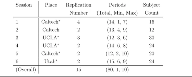
We conducted six experimental sessions, with the participant number ranging between 12 and 30. Three sessions were conducted at Caltech, two at UCLA, and one at the University of Utah. This generated 80 periods in total, spread over 15 replications. Table 4 provides specifics. Our novel termination protocol was applied in all sessions. The starred sessions ended with a period in which participants knew for sure that it was the last one, and hence, generated no trade.
We first discuss volume, and then look at prices and choices.
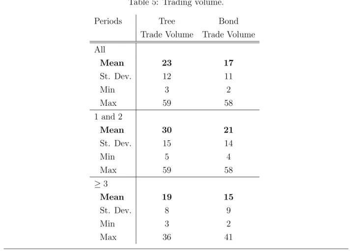
Volume. Table 5 lists average trading volume per period (excluding periods in which should be no trade). Consistent with theoretical predictions, trading volume in Periods 1 and 2 is significantly higher; it reflects trading needed for agents to move to their steady-state holdings. In the theory, subsequent trade takes place only to smooth consumption across odd and even periods. Volume in the Bond is significantly lower in Periods 1 and 2. This is an artefact of the few replications when the state in Period 1 was low. It deprived Type I participants of cash (Type I participants start with 10 Trees and no income). In principle, they should have been able to sell enough Trees to buy Bonds, but evidently they did not manage to complete all the necessary trades in 10Because both assets are in positive supply, our economy is an example of a Lucas orchard economy
Table 4: Summary data, all experimental sessions.
Session Place Replication Periods Subject
Number (Total, Min, Max) Count
1 Caltech∗ 4 (14, 1, 7) 16 2 Caltech 2 (13, 4, 9) 12 3 UCLA∗ 3 (12, 3, 6) 30 4 UCLA∗ 2 (14, 6, 8) 24 5 Caltech∗ 2 (12, 2, 10) 20 6 Utah∗ 2 (15, 6, 9) 24 (Overall) 15 (80, 1, 10)
the alotted time (four minutes). Across all periods, 23 Trees and 17 Bonds were traded on average. With an average supply of 210 securities of each type, this means that roughly 10% of available securities was turned over each period.11 Overall, the sizeable volume is therefore consistent with theoretical predictions. To put this differently: we designed the experiment such that it would be in the best interest for subjects to trade every period, and subjects evidently did trade a lot.
Cross-Sectional Price Differences. Table 6 displays average period transaction prices as well as the period’s state (“High” if the dividend of the Tree was $1; “Low” if it was $0). Consistent with the Lucas model, the Bond is priced above the Tree, with the price differential (the dollar equity premium) of about $0.50. When checking against Table 1, this reflects a (constant relative) risk aversion aversion coefficient of 1 (i.e., logarithmic utility).
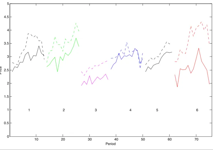
Prices Over Time. Figure 2 shows a plot of the evolution of (average) prices over time, arranged chronologically by experimental sessions (numbered as in Table 4); replications within a session are concatenated. The plot reveals that prices are volatile. In theory, prices should move only because of variability in economic fundamentals, which in this case amounts to changes in the dividend of the Tree. Specifically, prices should be high in High states, and low in Low states. In reality, much more is going on; prices are credpb excessively volatile. In particular, contrary to the Lucas model, price drift can be detected. Still, the direction of the drift is not obvious; the drift appears to be stochastic.
11Since trading lasted on average 210 seconds each period, one transaction occurred approximately every
Table 5: Trading volume.
Periods Tree Bond
Trade Volume Trade Volume
All Mean 23 17 St. Dev. 12 11 Min 3 2 Max 59 58 1 and 2 Mean 30 21 St. Dev. 15 14 Min 5 4 Max 59 58 ≥ 3 Mean 19 15 St. Dev. 8 9 Min 3 2 Max 36 41
Table 6: Period-average transaction prices and corresponding ‘equity premium’.
Tree Bond ‘Equity
Price Price Premium’
Mean 2.75 3.25 0.50
St. Dev. 0.41 0.49 0.40
Min 1.86 2.29 -0.20
Table 7: Mean period-average transaction prices and corresponding dollar equity premium, as a function of state.
State Tree Bond Equity Premium
Price Price (Dollar)
High 2.91 3.34 0.43
Low 2.66 3.20 0.54
Difference 0.24 0.14 -0.11
Nevertheless, behind the excessive volatility, evidence in favor of the Lucas model emerges. As Table 7 shows, prices in the high state are on average 0.24 (Tree) and 0.14 (Bond) above those in the low state. That is, prices do appear to move with fundamentals (dividends). The table does not display statistical information because (average) transaction prices are not i.i.d., so that we cannot rely on standard t tests to determine significance. We will provide formal statistical evidence later on, taking into account the stochastic drift evident from Figure 2.12
Cross-Sectional And Time Series Price Properties Together. While prices in High states are above those in Low ones, the differential is small compared to the size of the dollar equity premium. The average equity premium of $0.50 corresponds to a coefficient of relative risk aversion of 1, as mentioned before. This level of risk aversion would imply a price differential across states of $0.83 and $1.03 for the Tree and Bond, respectively. See Table 1. In the data, the price differentials amount to only $0.24 and $0.14. In other words, the co-movement between prices and fundamentals is lower than implied by the cross-sectional differences in prices between securities.
Still, the theory also states that the differential in prices between High and Low states should increase with the dollar equity premium. Table 8 shows that this is true in the experiments. The observed correlation is not perfect (unlike in the theory), but marginally significant for the Tree; it is insignificant for the Bond.
Prices: Formal Statistics. To enable formal statistical statements about the price differences across states, we ran a regression of period transaction price levels 12Table 7 also shows that the dollar equity premium is higher in periods when the state is Low than when
it is High. This is inconsistent with the theory. The average level of the dollar equity premium reveals logarithmic utility, and for this type of preferences, the equity premium should be lower in bad periods; see Table 1. This prediction is true for other levels of risk aversion too, but for lower levels of risk aversion, the difference in dollar equity premium across states is hardly detectible.
Table 8: Correlation between dollar equity premium (average across periods) and price differential of tree and bond across High and Low states.
Tree Bond
Correlation 0.80 0.52
(St. Err.) (0.40) (0.40)
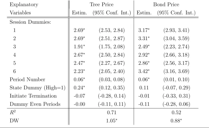
onto the state (=1 if high; 0 if low). To adjust for time series dependence evident in Figure 2, we added session dummies and a time trend (Period number). In addition, to gauge the effect of our session termination protocol, we added a dummy for periods when we announce that the session is about to come to a close, and hence, the period is either the penultimate or last one, depending on the draw of the die. Lastly, we add a dummy for even periods. Table 9 displays the results.
We confirm the positive effect of the state on price levels. Moving from a Low to a High state increases the price of the Tree by $0.24, while the Bond price increases by $0.11. The former is the same number as in Table 7; the latter is a bit lower. The price increase is significant (p = 0.05) for the Tree, but not for the Bond.
The coefficient to the termination dummy is insignificant, suggesting that our termi-nation protocol is neutral, as predicted by the Lucas model. This constitutes comforting evidence that our experimental design was correct.
Closer inspection of the properties of the error term did reveal substantial depen-dence over time, despite our including dummies to mitigate time series effects. Table 9 shows Durbin-Watson (DW) test statistics with value that correpond to p < 0.001.
Proper time series model specification analysis revealed that the best model involved first differencing price changes, effectively confirming the stochastic drift evident in Figure 2 and discussed before. All dummies could be deleted, and the highest R2 was obtained when explaining (average) price changes as the result of a change in the state. See Table 10.13 For the Tree, the effect of a change in state from Low to High is a significant $0.19 (p < 0.05). The effect of a change in state on the Bond price remains insignificant, however (p > 0.05). The autocorrelations of the error terms are now acceptable (marginally above their standard errors).
At 18%, the explained variance of Tree price changes (R2) is high. In theory, 13We deleted observations that straddled two replications. Hence, the results in Table 10 are solely based
on intra-replication price behavior. The regression does not include an intercept; average price changes are insignificantly different from zero.
Table 9: OLS regression of period-average transaction price levels on several explanatory
variables, including state dummy. (∗ = significant at p = 0.05; DW = Durbin-Watson
statistic of time dependence of the error term.)
Explanatory Tree Price Bond Price
Variables Estim. (95% Conf. Int.) Estim. (95% Conf. Int.)
Session Dummies: 1 2.69∗ (2.53, 2.84) 3.17∗ (2.93, 3.41) 2 2.69∗ (2.51, 2.87) 3.31∗ (3.04, 3.59) 3 1.91∗ (1.75, 2.08) 2.49∗ (2.23, 2.74) 4 2.67∗ (2.50, 2.84) 2.92∗ (2.66, 3.18) 5 2.47∗ (2.27, 2.67) 2.86∗ (2.56, 3.17) 6 2.23∗ (2.05, 2.40) 3.42∗ (3.16, 3.69) Period Number 0.06∗ (0.03, 0.08) 0.06∗ (0.01, 0.10)
State Dummy (High=1) 0.24∗ (0.12, 0.35) 0.11 (-0.07, 0.29)
Initiate Termination -0.07 (-0.28, 0.14) -0.01 (-0.33, 0.31)
Dummy Even Periods -0.00 (-0.11, 0.11) -0.11 (-0.28, 0.06)
R2 0.71 0.52
DW 1.05∗ 0.88∗
Table 10: OLS regression of changes in period-average transaction prices. (∗ = significant
at p = 0.05.)
Explanatory Tree Price Change Bond Price Change
Variables Estim. (95% Conf. Int.) Estim. (95% Conf. Int.)
Change in State Dummy
(None=0; High-to-Low=-1, 0.19∗ (0.08, 0.29) 0.10 (-0.03, 0.23)
Low-to-High=+1)
R2 0.18 0.04
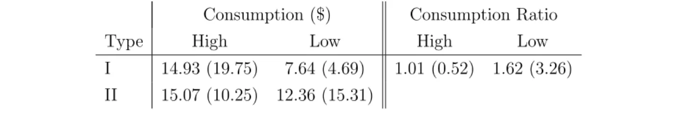
Table 11: Average consumption (end-of-period cash holdings) as a function of participant Type and State. Autarky numbers in parentheses.
Consumption ($) Consumption Ratio
Type High Low High Low
I 14.93 (19.75) 7.64 (4.69) 1.01 (0.52) 1.62 (3.26)
II 15.07 (10.25) 12.36 (15.31)
one should be able to explain 100% of price variability. But prices are excessively volatile, as already discussed in connection with Figure 2. Overall, the regression in first differences shows that, consistent with the Lucas model, fundamental economic forces are behind price changes, significantly so for the Tree. But at the same time, prices are excessively volatile, with no distinct drift.
Figure 3 displays the evolution of price changes, after chronologically concatenating all replications for all sessions. Like in the data underlying the regression in Table 10, the plot only shows intra-replication price changes. The period state (=1 if Low; 2 if High) is plotted on top.
Consumption Across States. Prediction 4 of the Lucas model states that agents of both types should trade to holdings that generate high consumption in High states, and low consumption in Low states. Assuming identical preferences, they should con-sume a fixed fraction of total period cash flows, or the ratio of Type I to Type II consumption should be equal in both states. The left-hand panel of Table 11 displays the average amount of cash (consumption) per type in High vs. Low states.14 In paren-theses, we indicate consumption levels assuming that agents do not trade (i.e., under an autarky). The statistics in the table confirm that consumption of both types increases with dividend levels. The result is economically significant because consumption is anti-correlated under autarky. This is strong evidence in favor of Lucas’ model.
Notice that under autarky (numbers in parentheses), consumption is anti-correlated across subject types. Type I subjects consume more in the High than in the Low state, and vice versa for Type II subjects. We deliberately picked parameters for our experiment to generate this autarky outcome, to contrast it with the (Pareto-optimal) outcome of the Lucas model, which predicts that consumption would become positively correlated.
14To compute these averages, we ignored Periods 1 and 2, to allow subjects time to trade from their initial
Table 12: Average consumption (end-of-period cash holdings) as a function of participant and period Types.
Consumption ($)
Type Odd Even
I 7.69 (2.41) 13.91 (20.65)
II 14.72 (20) 11.74 (5)
The right panel of Table 11 displays Type II’s consumption as a ratio of Type I’s consumption. The difference is substantially reduced from what would obtain under autarky (which is displayed in parentheses). Again, this supports the Lucas model, though the theory would want the consumption ratios to be exactly equal across states if preferences are the same.
Consumption Across Odd And Even Periods. Our fourth prediction is that subjects should be able to perfectly offset income differences across odd and even peri-ods. Table 12 demonstrates that our subjects indeed managed to smooth consumption substantially; the outcomes are far more balanced than under autarky (in parentheses; averaged across High and Low states, excluding Periods 1 and 2).15
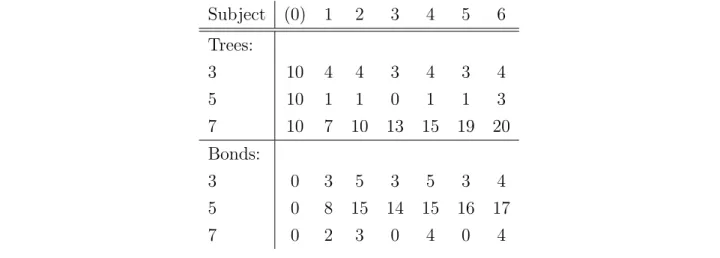
Price Hedging. The above results suggest that our subjects (on average) managed to move substantially towards (Pareto-optimal) equilibrium consumption patterns in the Lucas model. However, contrary to model prediction, they did not resort to price hedging as a means to ensure those patterns. Table ?? displays average asset holdings across periods for Type I subjects (who receive income in even periods). They are net sellers of assets in periods of income shortfall (see “Total” row), just like the theoretical agents with logarithmic utility (see Table 3). But unlike in the theoretical model, subjects decrease Tree holdings in low-income periods and increase them in high-income periods (compare to Table 3). As a by-product, Type I subjects generate cash mostly through selling Trees as opposed to exploiting the price differential between the Bond and the Tree. Only in period 9 is there some evidence of price hedging: Type I subjects on average buy Trees when they are income-poor (Period 9’s holding of Trees is higher than Period 8’s).
Altogether, it appears that the findings from our experiments are in line with the 15Autarky consumption of Type II subjects is not affected by states, because they are endowed with Bonds
which always pay $0.50 in dividends. In contrast, autarky consumption of Type I subjects depends on states. We used the sequence of realized states across all the sessions to compute their autarky consumption.
Table 13: End-Of-Period Asset Holdings Of Three Randomly Chosen Type I Subjects. Initial allocation is listed in column (0), for reference. Data from one replication in the first Caltech session. Subject (0) 1 2 3 4 5 6 Trees: 3 10 4 4 3 4 3 4 5 10 1 1 0 1 1 3 7 10 7 10 13 15 19 20 Bonds: 3 0 3 5 3 5 3 4 5 0 8 15 14 15 16 17 7 0 2 3 0 4 0 4
predictions of the Lucas model, with two exceptions: (i) prices were excessively volatile; (ii) subjects did not engage in price hedging.
These two anomalies could be related. Subjects may actually have expected volatile prices with no relation to economic fundamentals. If so, they would rationally have perceived no need to hedge price risk. In the short time span of a typical replication, their beliefs could not easily be falsified because prices were indeed very noisy. Still, the beliefs are actually wrong, at least as far as the Tree is concerned – but this we ourselves discovered only after pooling the price behavior from all sessions.
Regarding choices, however, there are significant individual differences, reminiscent of the huge cross-sectional variation in choices in static asset pricing experiments that led to the development of the ε-CAPM (Bossaerts et al., 2007a). Table 13 illustrates how three randomly chosen subjects of the same type (Type I) end up holding vastly different portfolios of Trees and Bonds. Curiously, subject 7 increased his holdings of Trees over time. Significantly, this subject bought Trees even in periods with in-come shortfall (odd periods), effectively implementing the price hedging strategy of the theory. Subject 3 is almost a perfect agent, diversifying across Trees and Bonds. But Subject 3 does not resort to price hedging, because Tree holdings decrease in odd periods. The message to be drawn from the table should be clear: one ought not to draw conclusions about prices or allocations at the market level from merely observing a single individual. Conversely, it is difficult to find a subject whose choices “explain” prices.
5
Discussion
The experiments demonstrate that our design “delivers” in the sense that it generates meaningful results in line with the Lucas model, with the exception of the excessively volatile prices and the absence of concern for price hedging among subjects.
Here, we discuss how these two anomalies may actually be related.
To see how, remember that in our setting, for the Lucas pricing results to obtain, agents need to have perfect foresight of the equilibrium relationship between prices and dividends. That is, the Lucas pricing results are the outcome of a Radner equilibrium (Radner, 1972). An interesting question is whether small deviations from perfect fore-sight would have noticeable effects on equilibrium prices and allocations. As we shall see, the effect on prices is substantial; while the effect on allocations is minimal. The effect on prices was independently discovered in Adam et al. (2012), and proves useful to explain excess volatility in historical field data, just like we can use it to make sense of our experimental data.16
The absence of demand for (price) hedging may indeed reflect subjects’ belief that prices do not co-move with economic fundamentals. It seems that subjects expected prices to be a martingale, as if subjects believed in the naive version of the EMH that the Lucas model discredits. The belief is wrong, as we pointed out, but not readily falsifiable within the short time of an experiment, and even after 80 observations (80 periods), not falsifiable for Bond prices (see Table 10). That is, the belief is a credible working hypothesis.
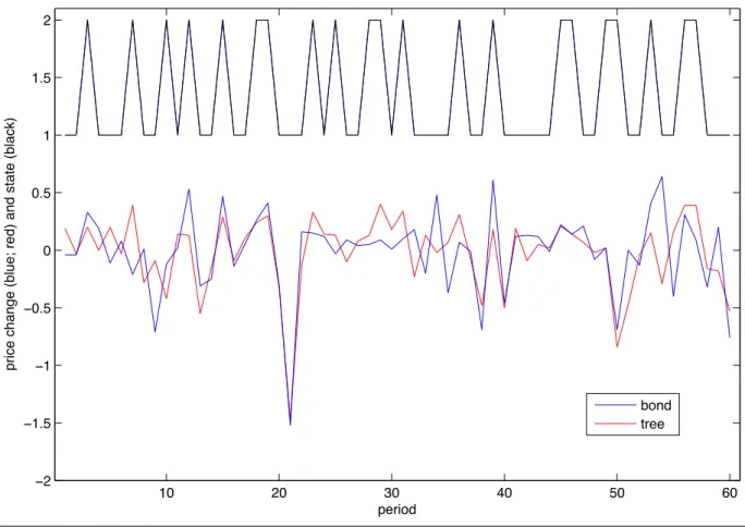
To determine the equilibrium effects of these beliefs, imagine that agents always ex-pect past prices to be best predictions of future prices, irresex-pective of future economic fundamentals. Given these beliefs, agents correctly solve their dynamic investment-consumption problem, send corresponding demands to markets, where prices are such that there is equilibrium each period. How would this equilibrium evolve over time? Simulations which we performed reveal that prices behave very much like in the exper-iment. They exhibit stochastic drift. While they do co-move with dividends, they are very noisy, and hence, excessively volatile. Figure 4 plots the evolution of the prices of 16Most analyses of belief mistakes in the context of the Lucas model have looked at false beliefs about the
(exogenous) economic fundamentals. See, e.g., Hassan and Mertens (2010). Adam et al. (2012) and ours are the only studies that focus exclusively on the endogenous aspects of a Lucas economy, namely, the mapping of states to prices. We claim that agents would have a much harder time learning about endogenous random variables – prices – than about exogenous random variables – dividends. In fact, in our experimental setting, subjects were told what the process of exogenous random variables was, while we left it to them to correctly anticipate future prices.
the Tree and Bond over the first 100 periods in one simulation. Plotted also are the state realizations (in red). The similarity with prices in our experiments (see Figure 2) is striking; the similarity was confirmed in formal statistical tests.
Importantly, just like in the experiments, excessive volatility makes it hard for one to reject the null that prices are unrelated to fundamentals. At conventional p levels (5%), it almost always takes 10 periods before detecting significant correlation between prices and fundamentals, and even then, the effect is only marginal economically, meaning that one may not want to implement the elaborate price hedging strategies that are required to generate the Lucas equilibrium.
Overall, then, beliefs are not far off the mark. Agents expect past prices to be best predictors of future prices, and these beliefs are almost confirmed in the resulting equilibrium. This is “almost” a Radner equilibrium (beliefs about prices are almost correct), yet prices are vastly different from the real Radner equilibrium (i.e., the Lucas model). Our exercise teaches that the Lucas model is not robust to slight mistakes in expectations about prices. As mentioned before, Adam et al. (2012) derived an analogous result, and showed that it provides a good rationale for excessive volatility of historical real-world stock market prices.
Interestingly, allocations in our “near” Radner equilibrium are close to Pareto op-timal, just like in the experiments. This is because agents invest correctly given their beliefs, and their beliefs are “near” correct. As such, “near” Radner equilibria may look vastly different from the Lucas outcome in terms of pricing, but generate nearly the same allocations. The message is clear: if welfare is the goal, excessive volatility is of little concern, as long as beliefs are nearly fulfilled, and agents correctly act on them.17
6
Conclusion
Over the last thirty years, the Lucas model has become the core theoretical model through which scholars of macroeconomics and finance view the real world, advise investments in general and retirement savings in particular, prescribe economic and financial policy and induce confidence in financial markets. Despite this, little is known about the true relevance of the Lucas model. The recent turmoil in financial markets 17Notice that our conclusion is diametrically opposed to that in Hassan and Mertens (2010), but this is
because the latter paper assumes that agents have incorrect beliefs about economic fundamentals. Instead, our agents have the right beliefs about fundamentals, and only slightly incorrect beliefs about equilibrium prices.
and the effects it had on the real economy has severely shaken the belief that the Lucas model has anything to say about financial markets. Calls are being made to return to pre-Lucas macroeconomics, based on reduced-form Keynesian thinking. This paper was prompted by the belief that proper understanding of whether the Lucas model (and the Neoclassical thinking underlying it) is or is not appropriate would be enormously advanced if we could see whether the model did or did not work in the laboratory.
Of course, it is a long way from the laboratory to the real world, but it should be kept in mind that no one has ever seen convincing evidence of the Lucas model “at work” – just as no one had seen convincing evidence of another key model of finance (the Capital Asset Pricing Model or CAPM) at work until the authors (and their collaborators) generated this evidence in the laboratory (Asparouhova et al., 2003; Bossaerts and Plott, 2004; Bossaerts et al., 2007a). The research provides absolutely crucial – albeit modest – evidence concerning the scientific validity of the core asset pricing model underlying formal macroeconomic and financial thinking.
Specifically, despite their complexity, our experimental financial markets exhibited many features that are characteristic of the Lucas model, such as the co-existence of a significant equity premium and (albeit reduced) co-movement of prices and economic fundamentals. Consistent with the model, the co-movement increased with the magni-tude of the equity premium. And subjects managed to smooth consumption over time and across states. Smoothing was not perfect, but sufficient for consumption to be-come positively correlated across subject types, consistent with Pareto optimality, and in sharp contrast with consumption under autarky, which was negatively correlated. Prices were excessively volatile though (not unlike in the real world, incidentally). And we did not observe price hedging, perhaps because subjects believed that the best pre-dictor for future prices were past prices (reminiscent of a naive version of EMH?). Still, such beliefs were not irrational: within the time frame of a single replication, there was insufficient evidence to the contrary, because the excess volatility made it hard to determine to what extent prices really reacted to fundamentals.
Overall, we view our experiments as a success for the Lucas model. Note that this model is only a reduced-form version of a general equilibrium. It assumes that markets somehow manage to reach Pareto optimal allocations, but is silent about how to get there. In our experiment, markets were incomplete, which makes attainment of Pareto optimality all the more challenging – markets had to be dynamically complete, and sophisticated trading strategies were required. Our design was in part mandated by experimental considerations: with incomplete markets, subjects had to trade every period. Crockett and Duffy (2010) have demonstrated that subjects need a serious
reason to trade in all periods, otherwise pricing anomalies (bubbles) emerge. But we would also argue that realistic markets are generically incomplete, and as such, our experiments provide an ecologically relevant test of the Lucas model.
Real-world financial markets are thought to be excessively volatile, and policy mak-ers have long been worried about this. On the policy side, our experimental results lead to a provocative conclusion: if welfare is the goal, excessive volatility is of little concern. This conclusion holds as long as beliefs are nearly fulfilled, and agents correctly act on them. The possibility that financial markets may be able to generate Pareto optimal outcomes in spite of excessive volatility has so far escaped the attention of empiricists and theorists, because evaluation of Pareto optimality cannot be performed on field data. Pricing had to be focused on, taking allocations as given. Experiments like ours, in contrast, allow one to study the optimality of allocations, and the interplay between prices and allocations.
Our experimental results also illustrate that it is dangerous to extrapolate from the individual to the market. As in our static experiments (Bossaerts et al., 2007b), we find substantial heterogeneity in choices across subjects; most individual choices have little or no explanatory power for market prices, or even for choices averaged across subjects of the same type (same endowments). Overall, the system (market) behaves as in the theory (modulo excessive price volatility), but the theory is hardly reflected in individual choices. As such, we would caution against developing asset pricing theories where the system is a mirror image of (one of) its parts. For instance, it is doubtful that prices in financial markets would reflect, say, prospect theoretic preferences (Barberis et al., 2001), merely because many humans exhibit such preferences (leaving aside the problem that these preferences do not easily aggregate). The “laws” of the (financial) system are different from those of its parts.
The next step in our experimental analysis should be to reduce the termination probability, thereby generating longer time series. This way, one could study to what extent markets eventually converge to the Lucas equilibrium. The reader may wonder why we have not done so already. One reason is experimental. We wanted to make sure that subjects understood that any period, including the first one, could be terminal. To be credible, we needed to generate a few cases where termination occurred early on (one of the replications in the first session terminated after one period, and we did not fail to mention this during the instruction phase of the subsequent sessions). This required a high termination probability. The second reason is based on personal
opinion. We do not believe that the real world is stationary. Parameters change
happens in Lucas economies of long duration. Despite the short horizon, we find it remarkable that our experimental markets manage to generate results that are very much in line with general equilibrium theory (suitably modified to explain the noise prices). Nevertheless, eventual convergence to the Lucas equilibrium is an interesting theoretical possibility, and here again, laboratory experiments could be informative.
Appendix: Instructions (Type I Only)
#$%!&''($))*!+,-./0(.12.-3$241$'56+76! 8)$(!9.7$*! :.));0('*! <=>?@8A?<B=>! "1 >,35.3,09! B9$!)$)),09!0+!34$!$CD$(,7$93!209),)3)!0+!.!957%$(!0+!($D-,2.3,09)!0+!34$!).7$!),35.3,09E! ($+$(($'!30!.)!!"#$%&'1!! F05!;,--!%$!.--02.3$'!'"()#$*$"'!34.3!G05!2.9!2.((G!34(05/4!.--!D$(,0')1!F05!;,--!.-)0!%$! /,H$9!(+',E!%53!2.)4!;,--!903!2.((G!0H$(!+(07!09$!D$(,0'!30!.9034$(1!! IH$(G!D$(,0'E!7.(J$3)!0D$9!.9'!G05!;,--!%$!+($$!30!*#+&"!G05(!)$25(,3,$)1!F05!%5G! )$25(,3,$)!;,34!2.)4!.9'!G05!/$3!2.)4!,+!G05!)$--!)$25(,3,$)1!! A.)4!,)!903!2.((,$'!0H$(!.2(0))!D$(,0')E!%53!34$($!;,--!%$!3;0!)05(2$)!0+!+($)4!2.)4!,9!.! 9$;!D$(,0'1!K,()3E!34$!)$25(,3,$)!G05!.($!40-',9/!.3!34$!$9'!0+!34$!D($H,05)!D$(,0'!7.G! D.G!&$-$&".&'1!?4$)$!',H,'$9')!%$207$!2.)4!+0(!34$!)5%)$L5$93!D$(,0'1!>$209'E!%$+0($! 34$!)3.(3!0+!)D$2,+,2!D$(,0')E!G05!7.G!%$!/,H$9!$.(%/"1!?4,)!,9207$!%$207$)!2.)4!+0(! 34$!D$(,0'1!<3!;,--!%$!J90;9!%$+0($4.9'!,9!;4,24!D$(,0')!G05!($2$,H$!,9207$1!! I.24!D$(,0'!-.)3)!M!7,953$)1!?4$!303.-!957%$(!0+!D$(,0')!,)!903!J90;9!%$+0($4.9'1! <9)3$.'E!.3!34$!$9'!0+!.!D$(,0'E!;$!'$3$(7,9$!;4$34$(!34$!$CD$(,7$93!2093,95$)E!.)! +0--0;)1!#$!34(0;!.!3;$-H$N),'$'!',$1!<+!34$!053207$!,)!O!0(!PE!;$!3$(7,9.3$!34$!)$)),091! B34$(;,)$!;$!2093,95$!.9'!.'H.92$!30!34$!9$C3!D$(,0'1!=03,2$*!34$!3$(7,9.3,09!24.92$! ,)!3,7$N,9H.(,.93Q!,3!'0$)!903!'$D$9'!09!40;!-09/!34$!$CD$(,7$93!4.)!%$$9!/0,9/1!! !"#$%&'(&$)*&+,%&-$+)+./%-$&%0&,&$*)+&0%12%,3&%4-/3%2"#%-$&%3"50)+.%-,%,3&%&+0% "6%,3&%(&$)"0%)+%73)43%,3&%/&//)"+%&+0/8%% >0E!,+!G05!$9'!.!D$(,0'!;,34053!2.)4E!.9'!;$!3$(7,9.3$!34$!)$)),09!.3!34.3!D0,93E!G05!;,--! 903!$.(9!.9G!709$G!+0(!34$!)$)),091!?4,)!'0$)!903!7$.9E!40;$H$(E!34.3!G05!)405-'! $9)5($!34.3!G05!.-;.G)!$9'!;,34!09-G!2.)4!.9'!90!)$25(,3,$)1!K0(!,9!34.3!2.)$E!,+!;$! 2093,95$!34$!$CD$(,7$93E!G05!;,--!903!($2$,H$!',H,'$9')E!.9'!4$92$E!G05!)3.(3!34$! )5%)$L5$93!D$(,0'!;,34053!2.)4!R.9'!90!)$25(,3,$)S!59-$))!34,)!,)!.!D$(,0'!;4$9!G05! ($2$,H$!,9207$1!!! #$!;,--!(59!.)!7.9G!)$)),09)!.)!2.9!%$!+,3!,9!34$!.--033$'!3,7$!0+!3;0!405()!+0(!34$! $CD$(,7$931!<+!34$!-.)3!)$)),09!;$!(59!4.)!903!%$$9!3$(7,9.3$'!%$+0($!34$!)24$'5-$'!$9'! 0+!34$!$CD$(,7$93!;$!;,--!3$(7,9.3$!34$!)$)),09!.9'!G05!;,--!$.(9!34$!2.)4!G05!.($! 40-',9/!.3!34.3!D0,931!! F05!;,--!%$!D.,'!34$!$.(9,9/)!0+!3;0!(.9'07-G!240)$9!)$)),09)1!<+!;$!7.9./$!30!(59! 09-G!09$!)$)),09!'5(,9/!34$!.--033$'!3,7$!+0(!34$!$CD$(,7$93E!G05!;,--!%$!D.,'!'05%-$!34$! $.(9,9/)!+0(!34.3!)$)),091! T5(,9/!34$!$CD$(,7$93E!.220593,9/!,)!'09$!,9!($.-!'0--.()1! !! "! "# $%&%! '()*)!+,--!.)!&+/!&01)2!/3!2)45*,&,)26!4%--)7!!"##!%87!$%&'#!98)!58,&!/3!&()!&*))!1%02!%! *%87/:!!"#"!$%!&'(&)$*'&'*&'%$&!'++,*6!+,&(!);5%-!4(%84)<!1%2&!7,=,7)872!(%=)!8/! ,83-5)84)!/8!&(,2!4(%84)#!>'()!%4&5%-!7*%+!,2!/.&%,8)7!52,8?!&()!2&%87%*7!12)57/@ *%87/:!85:.)*!?)8)*%&/*!,8!&()!1*/?*%:!A:%&-%.BC#!98)!58,&!/3!&()!./87!,+-,./&0,./& ("(1.&2$%1/#!D/5!+,--!*)4),=)!&()!7,=,7)872!/8!0/5*!(/-7,8?2!/3!&*))2!%87!./872!,8!4%2(! $#(%"#!%!8)+!1)*,/7!2&%*&2#!E2!254(6!0/5!+,--!*)4),=)!7,=,7)872!/8!0/5*!,8,&,%-!%--/4%&,/8! /3!&*))2!%87!./872!.)3/*)!&()!3,*2&!1)*,/7!2&%*&2#! D/5!+,--!2&%*&!&(,2!2)22,/8!+,&(!)*+!"##,+%87!*+$%&',#!9&()*2!:%0!2&%*&!+,&(!7,33)*)8&! ,8,&,%-!%--/4%&,/82#! F8!%77,&,/86!0/5!+,--!*)4),=)!,84/:)!)=)*0!%-&)*8%&)!1)*,/7#!F8!%''!1)*,/72!>G6HIC!0/5! +,--!*)4),=)!8/&(,8?6!%87!,8!#-#&!1)*,/72!>"6J6IC!0/5!+,--!*)4),=)!GK!7/--%*2#!'(,2! ,84/:)!,2!%77)7!&/!0/5*!4%2(!%&!&()!.)?,88,8?!/3!%!8)+!1)*,/7#!9&()*2!:%0!(%=)!%! 7,33)*)8&!,84/:)!3-/+#!! L)4%52)!4%2(!,2!&%M)8!%+%0!%&!&()!)87!/3!%!1)*,/7!+()8!&()!2)22,/8!7/)2!8/&!&)*:,8%&)6! &()!7,=,7)87!1%0:)8&2!0/5!*)4),=)6!&/?)&()*!+,&(!0/5*!,84/:)6!%*)!&()!2/-)!2/5*4)2!/3! 4%2(!3/*!%!8)+!1)*,/7#! H#!NO%:1-)2!>3/*!,--52&*%&,/8!/8-0C! '%.-)2!G!%87!"!?,=)!&+/!2%:1-)!)O%:1-)2!/3!/5&4/:)2!,8!%!2)22,/8#!F&!,2!%225:)7!&(%&! &()!2)22,/8!)872!%3&)*!&()!P&(!1)*,/7#!'%.-)!G!2(/+2!&()!%22)&!(/-7,8?26!7,=,7)87!%87!
4%2(!)%4(!1)*,/7!,3!&()!2&%&)2!%*)!%2!1)*!*/+!"!%87!&()!,87,=,75%-!2&,4M2!&/!&()!,8,&,%-! %--/4%&,/8!&(*/5?(/5&#!'()!3,8%-!&%M)@%+%0!4%2(Q)%*8,8?!,2!"K!7/--%*2!%2!&()!2)22,/8! &)*:,8%&)7!%3&)*!P&(!1)*,/7#!F&!+/5-7!(%=)!.))8!RS!,3!,&!(%7!&)*:,8%&)7!,8!1)*,/7!K#!
'%.-)!"!2(/+2!&()!4%2)!+()*)!&()!,87,=,75%-!&*%7)2!%2!3/--/+2T! • F8!1)*,/7!G6!&/!%8!%--/4%&,/8!/3!K!&*))2!%87!K!./8726!! • E87!25.2);5)8&-06!2)--,8?!&/!%4;5,*)!:/*)!4%2(!,3!7,=,7)872!%87!,84/:)!%*)! 7)):)7!&//!-/+6! • 9*!.50,8?!:/*)!%22)&2!+()8!7,=,7)872!%87!,84/:)!%*)!(,?(#!! U,84)!&()*)!,2!%!GQP!4(%84)!&(%&!&()!2)22,/8!)872!,8!&()!1)*,/7!+()8!%!2)45*,&0!,2!./5?(&6! ,&2!)O1)4&)7!=%-5)!);5%-2!>!!!!!!!!! C!&,:)2!&()!)O1)4&)7!7,=,7)87!>+(,4(!,2!);5%-!3/*!./&(! &()!&*))!%87!&()!./87C6!/*!>KC!V!>S#KC!W!"#KS#!'*%7)!,2!%225:)7!&/!&%M)!1-%4)!%&!"#KS#!X/&)6! (/+)=)*6!&(%&!&()!%4&5%-!&*%7,8?!1*,4)2!:%0!.)!7,33)*)8&6!%87!&(%&!&()0!:%0!)=)8!4(%8?)! /=)*!&,:)6!7)1)87,8?!/86!)#?#6!&()!7,=,7)87!/8!&()!&*))#!'()!3,8%-!&%M)@%+%0!4%2(!,8!&(,2! 4%2)!,2!RGK#SS#!F&!+/5-7!(%=)!.))8!RGH#SS!,3!&()!2)22,/8!(%7!&)*:,8%&)7!,8!1)*,/7!K#! ! !
! "! !"#$%&'(& PERIOD 1 2 3 4 5 6 State H L L H L H Initial Holdings Tree 10 10 10 10 10 10 Bond 0 0 0 0 0 0 Dividends Tree $1*10=10 $0*10=0 $0*10=0 $1*10=10 $0*10=0 $1*10=10 Bond $0.5*0=0 $0.5*0=0 $0.5*0=0 $0.5*0=0 $0.5*0=0 $0.5*0=0 Income 0 15 0 15 0 15 Initial Cash $10 (=10+0+0) $15 (=0+0+15) $0 (=0+0+0) $25 (=10+0+15) $0 (=0+0+0) $25 (=10+0+15) Trade Tree 0 0 0 0 0 0 Bond 0 0 0 0 0 0 Cash Change $0 $0 $0 $0 $0 $0 Final Holdings Tree 10 10 10 10 10 10 Bond 0 0 0 0 0 0 CASH $ 10.00 $ 15.00 $ 0.00 $ 25.00 $ 0.00 $ 25.00 ! !"#$%&)(& PERIOD 1 2 3 4 5 6 State H L L H L H Initial Holdings Tree 10 5 6 4 5 3 Bond 0 5 6 4 6 4 Dividends Tree $1*10=10 $0*5=0 $0*6=0 $1*4=4 $0*5=0 $1*3=3 Bond $0.5*0=0 $0.5*5=2.5 $0.5*6=3 $0.5*4=2 $0.5*6=3 $0.5*4=2 Income $0 $15 $0 $15 $0 $15 Initial Cash $10 (=10+0+0) $17.5 (=0+2.5+15) $3 (=0+3+0) $21 (=4+2+15) $3 (=0+3+0) $20 (=3+2+15) Trade Tree -5 +1 -2 +1 -2 +1 Bond +5 +1 -2 +2 -2 +1 Cash Change $0 -$5 +$10 -$7.5 +$10 -$5 Final Holdings Tree 5 6 4 5 3 4 Bond 5 6 4 6 4 5 CASH $ 10.00 $ 12.50 $ 13.00 $ 13.50 $ 13.00 $ 15.00 !
Appendix: Time Line Plot To Complement
In-structions
Period 1 Period 2 Period 3
Dividends
from initial allocation of “Trees” and “Bonds”
Income
Trade
to a final allocation of “Trees,” “Bonds,” and CASH
Possible Termination of Session *If termination--keep CASH *If continuation--lose CASH, carry over “Trees” and “Bonds”
Dividends
from carried over allocation of “Trees” and “Bonds”
Income
Trade
to a final allocation of “Trees,” “Bonds,” and CASH
Possible Termination of Session *If termination--keep CASH *If continuation--lose CASH, carry over “Trees” and “Bonds”
Etc.
References
Klaus Adam, Albert Marcet, and Juan Pablo Nicolini. Stock market volatility and learning. Working paper, 2012.
Elena Asparouhova, Peter Bossaerts, and Charles Plott. Excess demand and equi-libration in multi-security financial markets: The empirical evidence. Journal of Financial Markets, 6:1–21, 2003.
Ravi Bansal and Amir Yaron. Risks for the long run: A potential
reso-lution of asset pricing puzzles. The Journal of Finance, 59(4):1481–1509,
2004. ISSN 1540-6261. doi: 10.1111/j.1540-6261.2004.00670.x. URL
http://dx.doi.org/10.1111/j.1540-6261.2004.00670.x.
Nicholas Barberis, Ming Huang, and Tano Santos. Prospect theory and asset prices. The Quarterly Journal of Economics, 116(1):1–53, 2001. ISSN 00335533. URL http://www.jstor.org/stable/2696442.