A GPU implementation of Counterfactual Regret Minimization

(1)

F

ACULDADE DE

E

NGENHARIA DA

U

NIVERSIDADE DO

P

ORTO

A GPU implementation of

Counterfactual Regret Minimization

João Reis

Mestrado Integrado em Engenharia Informática e Computação

Supervisor: Henrique Lopes Cardoso (PhD)

Co-supervisor: Luís Teófilo (MSc)

(2)

(3)

A GPU implementation of Counterfactual Regret

Minimization

João Reis

Mestrado Integrado em Engenharia Informática e Computação

Approved in oral examination by the committee:

Chair: Daniel Augusto Gama de Castro Silva (PhD)

External Examiner: Paulo Jorge Freitas Oliveira Novais (PhD)

Supervisor: Henrique Daniel de Avelar Lopes Cardoso (PhD)

____________________________________________________

(4)

(5)

i

Abstract

Notable milestones in the advancement of Artificial Intelligence have been achieved through solving games. Regret minimization is a technique that has seen a lot of use in the context of solving games in the past few years. In particular, Counterfactual Regret Minimization (CFR) is an algorithm that applies this technique and can be used to find equilibria in massive games. Therefore, one can use an algorithm like this to develop an agent with a very solid strategy for such games.

One issue with this algorithm is the amount of execution time it requires, especially when applied to large extensive games. To address this issue, games are usually abstracted which can lead to worse solutions.

This dissertation proposes an implementation of CFR that runs on the GPU, using CUDA, which is able to take advantage of the ability of GPUs to process many parallel streams of data. Using this approach, it is possible to reduce the execution time in some Poker variants, as our results demonstrate. This means that this approach has the potential to allow the computation of Nash Equilibria for games with a larger search space than before.

(6)

(7)

iii

Resumo

Marcos notáveis no avanço da Inteligência Artificial foram alcançados através da obtenção de soluções para jogos. A técnica da Minimização do Arrependimento tem sido muito usada no contexto da obtenção de soluções para jogos nos últimos anos. Em particular, Counterfactual Regret Minimization (CFR) é um algoritmo que aplica esta técnica e pode ser usado para encontrar equilíbrios em jogos massivos. Portanto, pode-se usar um algoritmo deste género para desenvolver um agente com uma estratégia muito sólida para esses jogos.

Um problema com este algoritmo é a quantidade de tempo de execução que exige, especialmente quando aplicada a jogos com enormes árvores de pesquisa. Para abordar este problema, os jogos são geralmente abstraídos o que pode levar a soluções piores.

Esta dissertação propõe uma implementação do CFR que corre no GPU, usando CUDA, que é capaz de tirar partido da capacidade de GPUs para processar elevadas quantidades de dados de forma paralela. Usando esta abordagem, é possível reduzir o tempo de execução em algumas variantes de Poker, como demonstram os resultados. Isto significa que este método tem o potencial de permitir o cálculo de Equilíbrios de Nash para jogos com um espaço de pesquisa maior do que antes.

(8)

iv

(9)

v

Acknowledgements

I would like to express my gratitude to my supervisor, MSc Luís Teófilo, for all the precious help he’s given me from the very first day of this entire process, especially during the times I was feeling a little lost. This dissertation would not exist today without his guidance.

I would also like to thank my other supervisor, PhD Henrique Lopes Cardoso, for his important part in the final document review.

I also want to thank my family for the exceptional amount of support they provided. I’m very lucky to have a very patient family, especially my parents who spent the most time with me and always made sure I had everything I needed.

I must also acknowledge my friends, who were there for me when I was feeling exhausted and losing motivation.

(10)

(11)

vii

“A little more persistence, a little more effort, and what seemed hopeless failure may turn to glorious success.”

(12)

(13)

ix

5.1 Poker variant A ... 36 5.1.1 Memory usage ... 36 5.1.2 Execution time ... 36 5.2 Poker variant B ... 37 5.2.1 Memory usage ... 38 5.2.2 Execution time ... 38 5.3 Poker variant C ... 39 5.3.1 Memory usage ... 39 5.3.2 Execution time ... 40 5.4 Poker variant D ... 40 5.4.1 Memory usage ... 41 5.4.2 Execution time ... 41 5.5 Analysis of Results ... 42

Conclusions and Future Work ... 46

6.1 Conclusions ... 46

6.2 Future Work ... 47

References ... 49

Execution time measurements ... 52

A.1 Poker variant A ... 52

A.1.1 Singlethreaded Recursive CFR ... 52

A.1.2 Multithreaded Iterative CFR (CPU) ... 52

A.1.3 Multithreaded Iterative CFR (GPU) ... 53

A.2 Poker variant B ... 53

(15)

xi

A.3 Poker variant C ... 54

A.3.3 Multithreaded Iterative CFR (GPU) ... 55

A.4 Poker variant D ... 56

(16)

(17)

xiii

List of Figures

Figure 1: Matrix of a two player strategic game in which each player has two

strategies [13] 7

Figure 2: Portion of the extensive-form game representation of three-card Kuhn with

jack (J), queen (Q) and king (K) as its three cards [6] 8

Figure 3: Matrix for the Prisoner's Dilemma game [2] 8

Figure 4: Slide taken from NVIDIA’s presentation on CUDA: "Small Changes, Big

Speed-up" [14] 10

Figure 5: Implementation of SAXPY in C [15] 11

Figure 6: CUDA implementation of SAXPY in C [15] 11

Figure 7: CUDA Memory Hierarchy 12

Figure 8: Part of the game tree of a Poker game (example) 17

Figure 9: Text file that defines a game of 3 player Kuhn limit poker 23 Figure 10: Small example of a game tree in this implementation 24 Figure 11: Example of the average strategies array in its initial state for a game with 2

sequences and 2 buckets 25

Figure 12: CFR training function 25

Figure 13: Summarized version of cfr() 26

Figure 14: Example that shows the probabilities array and strategy for two sequences. 27 Figure 15: Example of probabilities array in the iterative version of CFR 28 Figure 16: Example of the new array, sequencesPerLevel, for the same game

that is represented in Figure 10 29

Figure 17: Phase 1 of the multithreaded iterative version of CFR (summarized) 29 Figure 18: Phase 2 of the multithreaded iterative version of CFR (summarized) 30 Figure 19: Difference of sequence numbers in each version of CFR 30

Figure 20: Fetching data from a CUDA texture 32

Figure 21: Part of the first kernel that shows how the average strategy is updated using

shared memory 33

Figure 22: Game definition file for variant A 36

Figure 23: Execution times of the three implementations for variant A 37

(18)

xiv

Figure 25: Execution times of the three implementations for variant B 38

Figure 26: Game definition file for variant C 39

Figure 27: Execution times of the three implementations for variant C 40

Figure 28: Game definition file for variant D 40

Figure 29: Execution times of the three implementations for variant D 41

Figure 30: Reasons why the first phase kernel is not faster 43

(19)

(20)

(21)

xvii

List of Tables

Table 1: Matrix for a Rock-Paper-Scissors game where players bet one dollar each 16

Table 2: Some details about the game trees of each variant 35

Table 3: Memory usage of all implementations for variant A 36

Table 4: Memory usage of all implementations for variant B 38

Table 5: Memory usage of all implementations for variant C 39

Table 6: Memory usage of all implementations for variant D 41

Table 7: Measurements in seconds of singlethreaded recursive CFR with variant A 52 Table 8: Measurements in seconds of multithreaded iterative CFR (CPU) with variant

A 52

Table 9: Measurements in seconds of multithreaded iterative CFR (GPU) with variant

A 53

Table 10: Measurements in seconds of singlethreaded recursive CFR with variant B 53 Table 11: Measurements in seconds of multithreaded iterative CFR (CPU) with

variant B 54

Table 12: Measurements in seconds of multithreaded iterative CFR (GPU) with

variant B 54

Table 13: Measurements in seconds of singlethreaded recursive CFR with variant C 54 Table 14: Measurements in seconds of multithreaded iterative CFR (CPU) with

variant C 55

Table 16: Measurements in seconds of singlethreaded recursive CFR with variant D 56 Table 17: Measurements in seconds of multithreaded iterative CFR (CPU) with

variant D 56

(22)

xviii

(23)

xix

Abbreviations

CFR Counterfactual Regret Minimization GPU Graphics Processing Unit

CPU Central Processing Unit CUDA

RMA GPGPU OpenMP

Compute Unified Device Architecture Regret Minimization Agent

General Purpose Computing on Graphics Processing Units Open Multi-Processing

(24)

(25)

1

Chapter 1

Introduction

2

1.1 Context

To solve games of incomplete information, a solution concept called Nash equilibrium is 4

typically used. However, it is not feasible to compute or store these solutions for massive games such as Poker though it is possible to do it with approximations of Nash equilibria.

6

Regret Minimization Agents are agents that are used nowadays to compute such approximations of Nash equilibria for games with a large search space. These agents focus on 8

minimizing the regret, i.e., the difference between the actual payoff and the payoff that would have been obtained if a different course of action had been chosen.

10

It turns out that there is a well-known connection between regret and the Nash Equilibrium concept. This was proven by having two agents of this type competing against each other and 12

observing that both strategies converged to an approximation of a Nash Equilibrium. In light of this, it is possible to use an algorithm like Counterfactual Regret Minimization (CFR) to 14

develop an agent with a solid strategy, i.e., a conservative strategy that does not focus on maximizing the gains against a specific opponent but shows good results against any type of 16

opponent.

1.2 Motivation

18

The current state of the art algorithm for regret minimization – CFR – has some issues. The main issue is the fact that it requires a lot of computing resources and execution time. One way 20

of trying to address this issue is to come up with abstractions of complex games. However, this leads to solutions of worse quality. Another way to try to solve this problem is by parallelizing 22

(26)

Introduction

2

CPUs are quite limited on the number of cores they possess. This is not true for GPUs though, which are well-known for their heavy parallel processing and fast arithmetic operations. This 2

leads us to believe that GPUs should definitely be taken into consideration when optimizing an algorithm like CFR.

4

There is no known CFR implementation that takes advantage of the power that GPUs offer, at the moment. There is a high probability that such implementation would speed up the 6

algorithm to the point where it would be possible to develop strategies that are more solid and closer to a real Nash Equilibrium, as opposed to an approximation of one. This would be a result 8

of requiring less amount of abstraction due to having a faster algorithm.

1.3 Objectives and Hypothesis

10

The main goal of this dissertation is to find out if a GPU implementation of CFR can be more efficient than other existing implementations. If this turns out to be true, then, using such 12

implementation, it might be possible to solve abstractions of complex games faster than before or even reduce the amount of those abstractions.

14

The GPU implementation will be tested with different versions of Poker. Poker has a lot of variants, each one associated with different complexity and search tree size. Even a small 16

variant of two player Poker can have almost 1018_{game states (limit Texas Hold’em). Because}

of this, Poker has become a common measuring stick for performance in the context of finding 18

solutions for very large extensive games.

1.4 Structure of the Dissertation

20

Chapter 2 explains fundamental concepts that one must have knowledge of in order to better understand this dissertation. It contains two subchapters: Game Theory and GPGPU. The 22

first subchapter describes in detail several concepts of Game Theory that are used throughout this document and other publications in this area. The purpose of the second subchapter is to 24

provide basic information about what GPGPU is and how it is going to be used in the context of this dissertation.

26

Related work is included in Chapter 3, which provides a brief review of existing literature in the same area, including existing CFR implementations.

28

Chapter 4 explains the three implementations that were developed during this dissertation: Recursive CFR, CPU Multithreaded CFR and GPU Multithreaded CFR.

30

Chapter 5 details the experiments that were made on each implementation and provides some analysis for the results.

32

(27)

Introduction

(28)

4

Chapter 2

Background

2

This dissertation requires the knowledge of some game theory concepts. In this chapter, these will be explained briefly with examples.

4

It also requires basic understanding of parallel computing with focus on CUDA, which will also be briefly introduced in this chapter.

6

2.1 Game Theory

Game theory is applied in the study of decision problems that can be modelled by games. 8

This theory assumes that decision makers are rational, reason strategically and focus on maximizing their own utility.

10

Utility is essentially a number that represents the motivation of a player associated with a

certain outcome. This means that they make decisions which help them achieve certain 12

objectives and take into account the behavior of other decision makers.

2.1.1 Strategy and Strategy profiles

14

A move is an action that can be made by a player during a game and alters the game state. An example would be a player moving one of his or her pieces in chess from a square to another 16

square during his or her turn.

A strategy defines which moves should be made by a player. Therefore, a strategy is an 18

algorithm that tells the player what to do for every possible situation that can happen in a game. A strategy can be pure or mixed.

(29)

Background

5

In very simple games, a pure strategy can be associated with a single action. In games with a temporal structure, a pure strategy can be a sequence of actions [1].

2

A mixed strategy defines the probability for each pure strategy that is available to a player. Because probabilities are continuous, there are infinite mixed strategies available to the player, 4

assuming there are always at least two pure strategies available.

Another concept that should be understood is that of a strategy profile. A strategy profile is 6

a set of strategies that contains only one strategy per player.

2.1.2 Cooperative and non-cooperative games

8

A game can be cooperative or non-cooperative.

In cooperative games, there is usually a system to ensure that commitments between 10

players are kept and decisions or actions are usually made by groups of players. In these types of games, there is competition between groups of players rather than between individual 12

players.

A non-cooperative game is a competition between individual players. It is possible for 14

players to cooperate in these types of games, but there is no system in place to ensure commitments are kept, which means that any cooperation is self-enforced.

16

There is a simpler way to define these types of games, using the concept of utility. In cooperative games, the utility is shared, i.e., players that cooperate with each other focus on 18

maximizing the utility that is shared between them. In non-cooperative games, utility is not shared between any player and players focus on maximizing their own utility.

20

For this dissertation, only non-cooperative games are relevant.

2.1.3 Zero-sum and non-zero-sum games

22

In a zero-sum game, a player’s gain of utility is exactly balanced by the loss of utility of other players. Following the same logic, a player’s loss of utility is also exactly balanced by the 24

gain of utility of other players. Games like these are called zero-sum due to the fact that if the total gains are added up and the total losses are subtracted, the result of this sum will be zero. 26

Naturally, in a non-zero-sum game, this sum will be less than or more than zero. A zero-sum game is also called a strictly competitive game.

(30)

Background

6

2.1.4 Sequential and simultaneous games

In sequential games, players have information related to previous moves made by other 2

players. It is important to note that this information may be perfect or imperfect. These two concepts will be explained in the next subsection.

4

In simultaneous games, players either make their moves simultaneously or later players have no knowledge of the moves made by earlier players, therefore making them effectively 6

simultaneous.

2.1.5 Perfect and imperfect information

8

In a game with perfect information, each player, when making a decision, is perfectly informed of all the events that have occurred until that moment. Chess is a good example of a 10

game with perfect information. In a game of chess, both players can see every piece on the board and their positions which means the game state is visible. Furthermore, a player has 12

knowledge of every move that has been made previously when deciding which move to make in his or her turn.

14

Games with imperfect information are the opposite, which means that the information available to each player is not complete. Most card games are of imperfect information. Because 16

of hidden information, some game states are indistinguishable. There is a key concept relevant to this dissertation that is related to hidden information wich is the concept of information set. 18

An information set is basically a set of game states that the player cannot tell apart.

Simultaneous games cannot be of perfect information because when a player is deciding 20

which move to make, the actions of the other players may or may not be known.

2.1.6 Representation of games

22

There are two main ways to represent non-cooperative games: extensive form and normal

form. Cooperative games are usually represented in the characteristic function form but, as

24

these are not relevant for this dissertation, this form of representation will not be explained. A game in normal form shows the strategies available to each player and the outcomes 26

associated with each possible strategy profile. An outcome is usually represented by its utility. An alternative name for the concept of utility is payoff. This form of representation can also be 28

called strategic form. Games in this form are sometimes referred to as strategic games. Normal-form games are simultaneous, so a strategic game can also be defined as a “model of a situation 30

(31)

Background

7

A normal form game is usually represented by a matrix. Figure 1 shows an example of this type of matrixes. In this example, 𝑝𝑛𝑥 is the payoff for player 𝑛 when he or she chooses strategy

2 𝑥.

The extensive form is used for games that have a time sequencing of moves. This form 4

shows the temporal sequence of moves and all the information that is available to each player when he has to make a decision [3]. Thus, in these games, in contrast with normal form games, 6

players can consider their plans of action whenever they reach a decision point [2].

Extensive form games are usually represented by decision trees. In this type of trees, each 8

node represents a state in the game in which a player has to make a decision. The payoffs are specified for each path of the tree in its respective leaf node. Figure 2 shows a portion of the 10

decision tree for a game called Kuhn Poker. This game is a simple 3-card poker game by Harold E. Kuhn. In Kuhn Poker, two players each bet 1 chip before cards are given to them. Three 12

cards are shuffled and each player is given one card. A player does not know which card his opponent has. Play starts with player 1. A player may pass or bet on his turn. A bet is composed 14

by an additional chip. If a player bets and the next player passes, in what is called a terminal pass, the play who made the bet gets all chips in the pot. If two passes or two bets are made 16

successively, the player with the highest card takes all chips in the pot.

2.1.7 Nash Equilibrium

18

Nash Equilibrium is “the most commonly used solution concept in game theory” [2]. It is a strategy profile composed by strategies that the players cannot improve upon unilaterally. 20

Figure 1: Matrix of a two player strategic game in which each player has two strategies [13]

(32)

Background

8

This solution concept is typically used in non-cooperative games with two or more players. A typical example of a game that can be used to demonstrate the concept of Nash 2

Equilibrium is the Prisoner’s Dilemma. In this game, there are two suspects for a crime that are held in two separate cells. Prisoners can choose to confess or not to confess. Based on this, 4

there are three situations that can happen:

 One prisoner confesses and the other does not – the one who confessed is freed and

6

used as witness against the other, who will receive a sentence of four years.

 Both prisoners confess – they both receive a sentence of three years.

8

 Neither prisoner confesses – both will receive a sentence of one year.

Figure 2: Portion of the extensive-form game representation of three-card Kuhn with jack (J), queen (Q) and king (K) as its three cards [6]

(33)

Background

9

The payoff of each strategy is four subtracted by the number of years the prisoner has to spend in prison, if he chooses that strategy. The strategies and their payoffs for this game are 2

represented in Figure 3.

This is a strategic game that is simultaneous and non-cooperative. There is only one 4

strategy profile that fits the definition of a Nash Equilibrium, which is the situation in which both prisoners confess with payoff of 1 to both prisoners. In this situation, neither player can 6

improve the outcome by changing his strategy unilaterally which means this is indeed a Nash Equilibrium.

8

2.2 Poker

Poker games are used in the experiments of this dissertation, so it is useful to know what 10

they are and some of their basic rules.

Poker is a family of sequential card games of imperfect information that involve betting. 12

These games are also zero-sum and non-cooperative. They vary in the number of cards dealt to each player, i.e., hole cards, and the number of shared cards, i.e., board cards. They can also 14

vary in the number of hidden cards in each player’s hands but this is not relevant for this dissertation because in every variant used in the experiments, all cards in the players’ hands is 16

hidden.

In Poker, the first round of betting may involve forced bets, i.e., blinds. The first player 18

bets and then action proceeds clockwise to the next player in the table. Players can match the previous bets of that round (call), increase the bet (raise) or forfeit (fold). The first player can 20

also choose to not bet anything, in what is known as a check. The next players can also check in these situations. Depending on the specific variant that is being played, a certain amount of 22

board cards are drawn from the deck in each round. When every player but one folds the

remaining player wins the pot. If the last round finishes and there is still more than one player 24

that has not folded, then a showdown occurs. In a showdown, the players that did not fold reveal their hole cards and evaluate their hands. The player with the best hand wins the pot. Specific 26

rules about what ranks a hand above another one are not explained here as they are not necessary for this dissertation.

28

In limit Poker variants, the size of bets are fixed and there is a maximum number of raises allowed for each player per round. In no-limit Poker variants, such limits do not exist and 30

players can even decide to all in, by placing the highest bet available to them. This dissertation will only cover limit Poker variants, because in no-limit variants players have an additional 32

decision to make – choosing the right amount to bet in each situation – which further increases the complexity of the game. Even without this additional decision, limit Poker variants can still 34

(34)

Background

10

be very complex. One example is limit Texas Hold’em, which is a two player limit Poker variant that has almost 1018_{game states.}

2

2.3 General Purpose Computing on Graphics Processing Units

GPGPU is an approach that consists of transferring the compute-intensive portion of an 4

application to the GPU while leaving the rest of the application running on the CPU. This process is represented in Figure 4.

6

CPUs contain a lot of hardware that perform control operations. This is necessary because CPUs were designed to be a generic piece of hardware that accept a wide variety of commands. 8

Since GPUs are not general purpose, they do not have to pay this price of control hardware. Instead, their design focuses on optimizing raw throughput.

10

2.3.1 Compute Unified Device Architecture (CUDA)

CUDA is a parallel computing platform and programming model invented by NVIDIA. It 12

is the dominant proprietary framework for those who wish to use the GPGPU approach.

In the CUDA programming model, code can be executed either on the CPU, which is the 14

host, or on the GPU, which is the device. Code that is executed on the host can access memory Figure 4: Slide taken from NVIDIA’s presentation on CUDA:

(35)

Background

11

on both the host and device. Code running on the host can also launch kernels, which are functions executed on the device. Kernels are declared with the __global__ specifier.

2

Figure 6 shows a CUDA implementation of SAXPY in C and Figure 5 shows a sequential implementation of SAXPY in C. SAXPY stands for “Single-Precision A•X Plus Y”. It is a 4

function that takes as input two vectors of 32-bit floats X and Y with N elements each, and a scalar value A. It multiplies each element X[i] by A and adds the result to Y[i]. SAXPY is a 6

good “hello world” example for parallel computation [4].

In the CUDA implementation of SAXPY, the input vectors are copied from host memory 8

to device memory before executing the kernel. Then, the kernel is executed by 4096 blocks of 256 threads, which is a total of 4096 × 256 = 1048576 threads (one thread per vector 10

element). After the kernel execution, the output vector is copied back to host memory from device memory. The optimal execution configuration (number of blocks and threads per block) 12

for a specific kernel can be found only by experimentation. In the case of the GPU Figure 5: Implementation of SAXPY in C [15]

(36)

Background

12

implementation of CFR, the optimal number of threads per block was found to be 64 and the number of blocks depend on the total number of threads needed by each Poker variant.

2

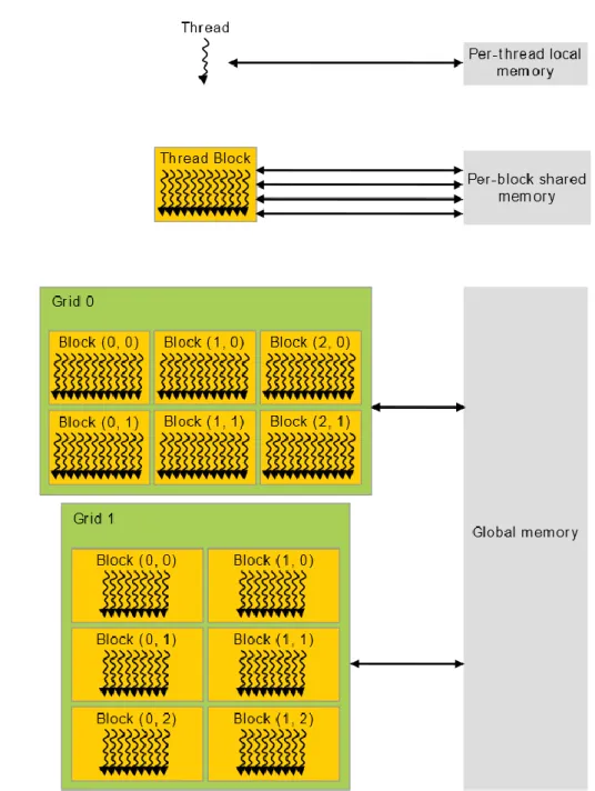
As this dissertation focuses on CUDA for the GPU implementation, it is also necessary to know and understand the different memory spaces that CUDA threads can access:

4

 Per-thread local memory – data is visible only to the thread that wrote it;

 Per-block shared memory – data is shared between all threads of the same block;

6

 Global memory – data is visible to all threads of the application, including the host.

Figure 7 illustrates the different types of memory in CUDA. 8

(37)

Background

13

There are two types of per-thread local memory: registers and local memory. Registers are used for automatic, i.e. local, variables declared within kernels. Local memory is used when 2

registers are not enough to hold all automatic variables. It is also used for automatic arrays. Shared memory is the only per-block shared memory type in CUDA. It can be used by 4

declaring a local variable or array with a __shared__ specifier within a kernel.

In the global scope, there are three different memory types: global, constant and texture. 6

Constant memory is used for data that is not changed throughout the execution of a kernel and is, therefore, read only. Texture memory is similar to constant memory as it is read only aswell 8

but is not limited to 64KB like constant memory is. Texture memory is optimized for 2D spatial locality. Both texture and constant memory are cached. Global memory is not cached and can be 10

modified by CUDA threads during kernel execution.

Regarding performance, registers are the fastest out of all memory types. Despite also 12

having thread scope, local memory is slow, because it is an abstraction of global memory. This means that local memory has the same performance as global memory. Shared memory is also 14

quite fast, second only to registers. Constant memory is slower than shared memory but faster than texture memory. Global memory and local memory are the slowest types in the CUDA 16

memory architecture but they are still needed in several situations.

2.3.2 CUDA and CFR

18

In this dissertation, CUDA is used in the implementation of the CFR algorithm that runs on the GPU. Chapter 3 explains what CFR is and Chapter 4 provides details about the 20

(38)

Background

(39)

15

Chapter 3

Related Work

2

3.1 Counterfactual Regret Minimization (CFR)

Extensive form is often used to represent sequential non-cooperative games, particularly 4

those with imperfect information. The usefulness of this model “depends on the ability of

solution techniques to scale well in the size of the model” [5]. Poker is one of the most

6

commonly used games when testing the performance of these solution techniques. One of the reasons that may be behind this success is the fact that even its small variants can be quite large. 8

For instance, heads-up limit Texas hold’em has 3.16 × 1017_{game states [6].}

Zinkevich et al. introduce the notion of counterfactual regret [5], which is applied in a new 10

technique for finding approximate solutions to large extensive games. An algorithm for minimizing counterfactual regret in poker was developed and used to solve poker abstractions 12

with as many as 1012_{games states, “two orders of magnitude larger than previous methods”}

[5]. 14

Counterfactual regret minimization extends the techniques of regret minimization and regret matching to sequential games. Neller and Lanctot use Kuhn Poker to explain the CFR

16

algorithm [7].

3.1.1 Regret matching and minimization

18

Regret is the difference between the utility of a certain action and the utility of the action

that was chosen. 20

Let´s consider the example given by Neller and Lanctot in order to better explain what regret minimization is: a game of Rock-Paper-Scissors where each player bets one dollar. The 22

(40)

Related Work

16

winner takes both dollars and, in case of a draw, players retain their dollars. The utilities of the strategies for both players are represented in Table 1.

2

Table 1: Matrix for a Rock-Paper-Scissors game where players bet one dollar each

Rock Paper Scissors Rock 0, 0 -1, 1 1, -1

Paper 1, -1 0, 0 -1, 1

Scissors -1, 1 1, -1 0, 0

Let’s say we have Player A and Player B who will play a round of this game. Player A plays Rock and Player B plays Paper, with B being therefore the winner. For this round, Player 4

A regrets not having played paper with value of 0 – (– 1) = 1 and regrets not having played scissors with value of 1 – (– 1) = 2. In the future, player A prefers to choose the action 6

associated with the highest value of regret, which is to play scissors. Note that this technique leaves player A predictable and thus exploitable which leads to the technique of regret 8

matching. Through regret matching, an agent’s actions are selected randomly according to a probability distribution that is proportional to positive regrets [5]. In the last example, Player A 10

has regret value of 0 for having chosen rock, 1 for not having chosen paper and 2 for not having chosen scissors. Now, let’s obtain the normalized positive regrets, i.e., positive regrets divided 12

by their sum: 0, 1 3⁄ and 2 3⁄ for rock, paper and scissors, respectively. With regret matching, Player A chooses his next action using the values obtained previously as probabilities. After the 14

next action is chosen and the round is complete, the next values of regret are known and it is possible to obtain the cumulative regrets which are the sum of the previous regret values. After 16

normalizing these cumulative regrets, Players would use these values as probabilities when choosing the next action.

18

In any two-player zero-sum game, when both players use regret-matching to update their strategies, their average strategies converge to a Nash equilibrium as the number of iterations 20

tends to infinite [5].

3.1.2 Counterfactual regret

22

Besides extending regret minimization and regret matching to sequential games, CFR introduces the concept of counterfactual regret, which is the regret weighted by the probability 24

of the opponent reaching the information set.

The basic principle behind CFR is the fact that, by minimizing the counterfactual regret at 26

(41)

Related Work

17

3.1.3 The original CFR algorithm

This algorithm is iterative. In each iteration, CFR plays one game and updates the 2

counterfactual regret values and mixed strategies for each information set according to the outcome of that game. Here is the basic steps that are performed for each information set, in one 4

iteration:

1. Compute expected utility of each action 6

2. Calculate the counterfactual regret for not taking each action 3. Add up counterfactual regret over all games of past iterations 8

4. Compute new strategy with probabilities that are proportional to the accumulated positive counterfactual regret values

10

To better explain how the algorithm works, consider an exemple of a Poker game. Part of the game tree is illustrated in Figure 8. At information set A, the current strategy is (1 4⁄ , 1 2⁄ , 12

1 4⁄ ), i.e., the probabilities of player calling, raising and folding are 1 4⁄ , 1 2⁄ and 1 4⁄ , respectively. The probability of the opponent reaching this information set is 1 2⁄ . When the 14

game reaches information set A, CFR will first compute the utility of each action: (4, 2, -3). Therefore, the strategy’s utility is 4 × 1 4 + 2 × 1 2⁄ ⁄ − 3 × 1 4⁄ = 1.25 . To obtain the 16

regret values, subtract each action’s utility by the strategy’s utility: (2.75, 0.75, -4.25). To obtain Figure 8: Part of the game tree of a Poker game (example)

(42)

Related Work

18

the counterfactual regret values, multiply the regret values by the probability of the opponent reaching the information set, i.e., 1 2⁄ : (1.375, 0.375, -2.125). Finally, to obtain the new mixed 2

strategy, divide each counterfactual regret value by the sum of the positive counterfactual regret values. The negative counterfactual regret values lead to a probability of zero in the new 4

strategy. So the probabilities of calling, raising and folding in the new strategy are 1.375 (1.375 + 0.375)⁄ = 0.786 , 0.375 (1.375 + 0.375)⁄ = 0.214 and 0, respectively. 6

Note that the strategies at each information set should be initialized with a uniform distribution. In the previous example the initialized strategies would be (1 3⁄ , 1 3⁄ , 1/3). This 8

means that in the first iteration of the algorithm every information set has the same strategy.

3.2 CFR variants

10

3.2.1 Monte Carlo CFR

Monte Carlo CFR reduces the time spent traversing the game tree in each iteration by 12

considering only a sampled portion of it [8]. There is a form of Monte Carlo style sampling called chance-sampling. Using this form of sampling, the algorithm obtains a single, sampled 14

sequence of actions and only traverses the portion of the game tree that corresponds to that sequence [8].

16

Different sampling techniques lead to different variations of Monte Carlo CFR algorithms. The original CFR algorithm without sampling is usually called “vanilla CFR” [8]. There are 18

three variants of chance sampling: Opponent-Public Chance Sampling, Self-Public Chance

Sampling and Public Chance Sampling. Johanson et al. demonstrated empirically that an

20

equilibrium approximation algorithm is more efficient on large games using Public Chance Sampling [9].

22

Since Monte Carlo CFR variants are not particularly relevant for this dissertation, they will not be explained here. Johanson et al. provide detailed explanations of them [9].

24

3.2.2 CFR-BR

Computing Nash Equilibrium strategies in large extensive-form games requires too much 26

memory and time to be tractable [10]. The standard approach to overcome this issue is to use abstractions in order to reduce the size of the game. However, it has been recently found that 28

this type of abstractions leads to the computation of Nash equilibria that can be really far from optimal strategies in the unabstracted games [10]. CFR-BR is an algorithm that finds optimal 30

(43)

Related Work

19

The algorithm leaves one player unabstracted and tries to find the optimal abstract strategy for the other player. Usually, this would not be possible because of the computational 2

requirements, but this algorithm overcomes these issues in two ways:

 The opponent is assumed to employ a best-response strategy on each iteration instead 4

of a no-regret strategy;

 CFR-BR uses sampling techniques when computing the best-response strategy, which 6

means that the resulting strategy is not an exact best-response strategy.

CFR-BR was used to compute the least exploitable strategy ever reported for the game of 8

heads-up limit Texas hold’em [10]. This game is explained in the next subsection.

3.2.3 CFR+ and Cepheus

10

Several games of perfect information have been solved in the past, like checkers. However,

“no nontrivial imperfect information game played competitively by humans has previously been

12

solved” [6].

Poker is a good example of a nontrivial imperfect information game that is played 14

competitively by humans. Texas hold’em is the most popular variant of Poker, nowadays. When this variant is played with two players, with fixed bet sizes and fixed number of raises, it is 16

called heads-up limit Texas hold’em.

In 2015, Bowling et al. announced that heads-up limit Texas hold’em is now essentially 18

weakly solved. This was enabled by a new algorithm called CFR+. Like CFR, CFR+ is an iterative algorithm that computes an approximation to a Nash equilibrium. Also just like CFR, 20

as the number of iterations grows, the computed solution gets closer and closer to a real Nash equilibrium [6].

22

Using CFR+, it is possible to solve extensive games with orders of magnitude larger than those that can be solved using other algorithms. While typical CFR implementations traverse 24

only portions of the game tree, CFR+, by contrast, traverses the entire game tree. Also, CFR+ uses a variant of regret matching called regret matching+. With regret matching+, values of 26

regret are constrained to be non-negative [6].

CFR+ requires less computation than state-of-the-art sampling CFR, while keeping its 28

potential of massive parallelization[6].

Cepheus is “the first computer program to play an essentially perfect game of poker” [11]. 30

Specifically, this program plays heads-up limit Texas hold’em. Cepheus learns to play poker by playing against itself, using CFR+.

(44)

Related Work

20

3.3 Summary

CFR is an algorithm commonly used to find approximate solutions to large extensive 2

sequential games. It uses the techniques of regret minimization and regret matching, while introducing a new concept of regret, i.e., counterfactual regret.

4

The original algorithm uses so much memory and time that it is necessary to use asbtractions in order to apply it to some very large games like some variants of Poker. However 6

these abstractions lead to computed solutions that are very far from being optimal strategies in the unabstracted games. To overcome these issues, several CFR variants have been proposed, 8

such as Monte Carlo CFR, CFR-BR and CFR+. Monte Carlo and CFR-BR were quite successful in improving the quality of solutions computed by the algorithm but these solutions 10

are still not Nash equilibria. CFR+ was a success as it managed to solve heads-up limit Texas hold’em but it took 4800 CPUs running during 68 days to achieve this [12].

12

This dissertation shows that it is possible to achieve good results with a GPU implementation of CFR. However, the previously mentioned variants were tested with an 14

enormous amount of computational resources and time while the GPU implementation of CFR was tested on a quite small scale. Chapter 4 provides details about the GPU implementation and 16

Chapter 5 describes the details and results of every experiment that was done in the context of this dissertation.

(45)

Related Work

(46)

22

Chapter 4

Proposed CFR Implementations

2

Three different implementations of CFR for Poker variants were developed in the context of this dissertation. The first one is recursive, singlethreaded and runs on the CPU. The second 4

one is iterative, multithreaded and runs on the CPU. The third one is iterative, multithreaded and runs on the GPU. All three implementations use a C module developed by the Computer Poker 6

Research Group, University of Alberta1_{. This module provides game logic related functions for}

almost any variant of Poker. The game’s rules can be provided to the module by a text file. It 8

was distributed as part of the server software used in the Annual Computer Poker Competition2_.

4.1 Game logic module

10

The informated related to the game’s rules is stored in a struct called Game and everything related to the state of the game is stored in a struct called State. To create a Game structure, the 12

file containing the game’s parameters must be provided. Figure 9 shows an example of a text file that defines a specific variant of Poker. It is possible to define several parameters of a Poker 14

game such as:

 numPlayers – number of players

16

 numRounds – number of rounds

 blind – blinds for each player

18

 raiseSize – fixed amount for a raise, only used in limit games

 firstPlayer – who is the first to perform an action

20

 maxRaises – maximum number of raises in a round

1_{http://poker.cs.ualberta.ca/}

(47)

Implementation

23

 numSuits – number of suits in the deck

 numRanks – number of ranks in the deck

2

 numHoleCards – number of hole cards for each player

 numBoardCards – number of public shared cards on the board

4

By changing each parameter in these files, it is easy to run each CFR implementation with a lot of poker variants, each one with a different level of difficulty and number of information 6

nodes.

4.2 Recursive CFR

8

4.2.1 Abstractions

Each possible hand is placed on a bucket, which is represented by an integer. The more 10

hands there are per bucket, the more abstracted the game is. Because it is possible to tweak the game parameters in order to obtain Poker variants of different complexity, no abstraction will be 12

used, though each hand is still represented by a bucket number.

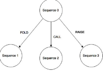
4.2.2 Game tree representation

14

In any Poker variant, there are at most three possible actions at any game state: fold, call and raise. Therefore, each node can have up to three child nodes. It is important to note that a 16

check is considered the same as a call in this implementation. A player will never fold if he can check, since there is a relationship of strategic dominance between the two.

18

(48)

Implementation

24

The class that represents a tree node is called Sequence. Every sequence object except the root has a parent Sequence. The root Sequence object represents the state in which no player has 2

taken any action yet. Figure 10 shows a very small example of a game tree that contains only four sequence objects, i.e., nodes. The Sequence class contains several fields that store 4

information about the game state in that node like current player, round number and number of possible actions available to the current player. Furthermore, there is a field that stores the 6

parent’s sequence number and a field that maps each possible action to a child Sequence.

It is important to note that this representation does not depend on anything related to the 8

deck that is used in the game. It only depends on the number of players, rounds and maximum number of raises. So if only the parameters related to the cards are changed in the game 10

definition files, then the Sequence objects will be identical. It is also important to note that an information set, in this context, is represented by a pair of one Sequence and one bucket. The 12

number of information sets in a certain game is equal to 𝑁𝑆𝐸𝑄𝑈𝐸𝑁𝐶𝐸𝑆× 𝑁𝐵𝑈𝐶𝐾𝐸𝑇𝑆 .

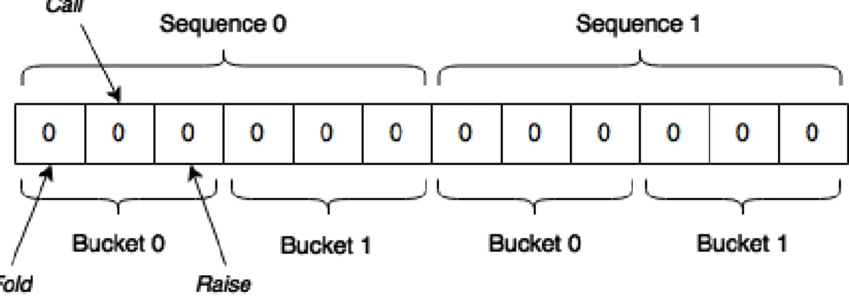
In the CFR algorithm, the average strategies and counterfactual regret values must be 14

stored and computed for each information set so the previous representation is not enough. At each Sequence, depending on the size of the deck, there are several possible hands that the 16

current player can have and each different hand corresponds to a different information set. Thus, the average strategies and counterfactual regret values are represented by arrays. An example of 18

such array can be seen in Figure 11. Note that there is one array for average strategies and another one for counterfactual regret values but both arrays have the same size and initial state. 20

(49)

Implementation

25

4.2.3 Brief explanation of core functions and variables

Figure 12 shows a summarized version of the main training function for this 2

implementation. The arrays average_strategy (line 2) and cfregret (line 3) are ones that were described in the previous section. The average strategy is basically the output of the 4

algorithm. The counterfactual regret values are stored in one iteration and used in the next so that is why there is a need for this array. The next array, utilitySum, is another output of the 6

algorithm (line 4) and it is used to measure the quality of the average strategy. It contains the sum of all utility values per player that were computed in each iteration (lines 13 – 14). By 8

dividing these sums by the number of iterations, the average utility is obtained.

Figure 11: Example of the average strategies array in its initial state for a game with 2 sequences and 2 buckets

(50)

Implementation

26

The function createSequences() creates an array of Sequence objects that holds every Sequence of the tree. The index of a certain Sequence is its sequence number.

2

The function initState(…) initializes a State struct to its initial default state while dealCards(…) modifies the State struct according to the game’s rules so that it contains 4

each player’s hands and also the board cards. The function that deals the cards determines the buckets for each player.

6

Finally, cfr(…) implements the recursive CFR for an iteration. Figure 13 shows a summarized version of this function. Each call is associated with a specific Sequence which 8

means that each execution of cfr(…) can lead to three more calls of the same function, one for each possible action in that Sequence. For each Sequence, the strategy is obtained through the 10

technique of regret matching as it was described in Chapter 3. Using this freshly obtained strategy, the average strategy for the current Sequence and bucket is updated. The strategy will 12

also be used to update the counterfactual regret values but this process also needs the utility values of each possible action. Now comes the recursive part: the utility values are returned by 14

this function which means that, in order to obtain the utility values for each action, a leaf Sequence node must be reached and the utility of this leaf node must be propagated back to 16

every parent node, including the root. In fact, this means that the last Sequence to have its counterfactual regret values updated will actually be the first one, i.e., root while being the first 18

one to have updated average strategies. Figure 13 does not show the part of the algorithm that returns the value of the state when the current Sequence has no actions possible, i.e., when it is a 20

leaf node.

(51)

Implementation

27

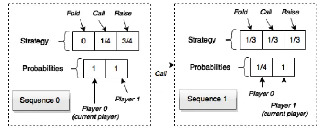
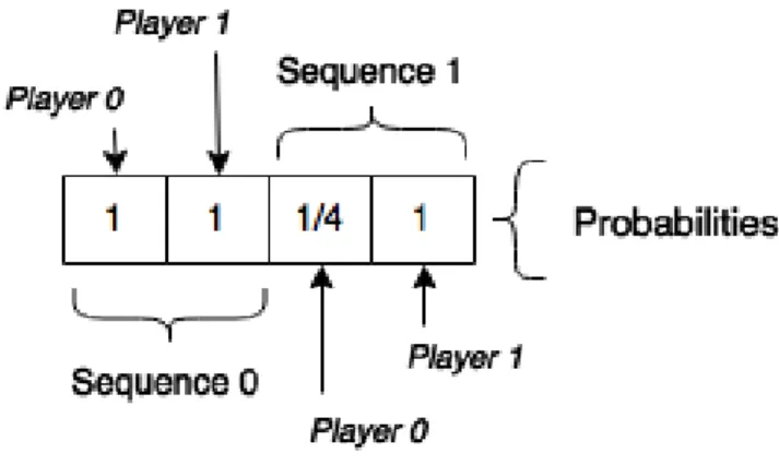
There is a parameter that has not been mentioned yet which is the probabilities array. As it was described in Chapter 3, CFR uses counterfactual regret – regret weighted by the 2

probability of the opponent reaching the information set. The probabilities array contains the probabilities of each player reaching the current sequence so that the counterfactual regret 4

can be computed.

Figure 14 shows the probabilities array and Strategy for an unspecified bucket in two 6

different sequences. Player 0 is the first to act, choosing to call. According to the strategy at that moment, Player 0 had 1 4⁄ probability of choosing that action, which leads to him having 8

probability 1 × 1 4⁄ = 1 4⁄ of reaching the information set represented in Sequence 1.

4.3 Iterative CFR

10

For the iterative version, it is necessary to split the algorithm into two different phases: 1. Update average_strategy and probabilities arrays for every sequence 12

in ascending order – first one to be updated is Sequence 0.

2. Update cfregret amd utilities array for every sequence in descending 14

order – first ones to be updated are the last sequences, i.e., leaf nodes.

This change could not be avoided because the values of counterfactual regret associated 16

with a sequence are dependent on every child sequence’s counterfactual regret values while the probabilities associated with a sequence are dependent on its parent sequence’s probabilities. In 18

the recursive version, the first phase is done before the recursive call and the second phase is done after the call.

20

Another change that must be done has to do with the probabilities array. This array has NPLAYERS elements in the recursive version because each function call passes a new array to

22

(52)

Implementation

28

the next call. In this iterative version, there is only one function call so there can only be one array for every Sequence. The new array has N_PLAYERS × NSEQUENCES elements. Figure 15

2

shows the probabilities array in the iterative version for the same game state as the one shown in Figure 14.

4

Similar to the situation with the probabilities, the State struct is passed by parameter in the recursive version so a new array must be used in the iterative version to store the State 6

associated with every Sequence. This new array has N_SEQUENCES elements.

The utility values are returned by each call in the recursive version so one more array is 8

declared in the iterative version where every player’s utility value is stored for every sequence. This new array, utilities, has N_PLAYERS × NSEQUENCES elements.

10

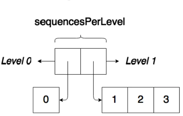
There is still one detail that is missing which is how to make this algorithm parallel. Consider the example shown in Figure 10: it is not possible to have the algorithm process 12

Sequence 0 and Sequence 1 at the same time because they depend on each other. However, once Sequence 0 is processed, it is possible to have all three child Sequences processed at the same 14

time since these do not depend on each other – each Sequence depends only on its parent and child Sequences. The way to make this algorithm parallel is to divide all Sequences in levels so 16

that every Sequence in the same level can be processed concurrently. Therefore we need one more array to make this possible, i.e., an array of arrays where the index is the level and the 18

array associated with the level contains every sequence number that belongs to that level. An example can be seen in Figure 16.

20

With this last change, the iterative version can be made parallel in both phases. In the first phase, the levels are processed in ascending order and in the second phase they are processed in 22

descending order.

(53)

Implementation

29

4.3.1 Multithreaded CPU Implementation

This implementation uses OpenMP, which is an API that supports multi-platform shared 2

memory multiprocessing programming in C++. OpenMP can be used to make a for loop parallel by only using a simple compiler directive. The API will be responsible for spawning threads 4

and dividing the iterations of the for loop between the available threads. It is also possible to choose how many threads are spawned. This is the only functionality of OpenMP that is needed 6

for this implementation.

The CPU implementation of the iterative version of CFR has many similarities with the 8

recursive implementation as it can be seen in Figure 17 and Figure 18. The inner for loop (line 3 in both Figures) is made parallel with the #pragma omp parallel for openMP 10

directive (line 2 in both Figures). In the actual implementation, there are some optimizations that were done so that this directive does not spawn and destroy threads in each iteration of the 12

outer for loop (line 1). Every important variable and array used in the CPU implementation of iterative CFR has been explained in the previous sections.

14

Figure 16: Example of the new array, sequencesPerLevel, for the same game that is represented in Figure 10

(54)

Implementation

30

There is an important optimization that has not been mentioned yet which considerably improves locality of reference when accessing the large arrays used in this iterative version. 2

This optimization consists of a change in order of Sequences in the game tree. This is illustrated by Figure 19. This optimization changes the structure of every array that is related to sequences 4

since sequences of the same level are close to each other in memory. In practice, the arrays are not actually different and what actually changes are the memory access patterns during the 6

execution of the algorithm.

Figure 18: Phase 2 of the multithreaded iterative version of CFR (summarized)

(55)

Implementation

31

4.3.2 Multithreaded GPU Implementation

Two CUDA kernels were implemented, one for each phase of the iterative CFR. It is very 2

similar to the CPU implementation, except for the arrays. Some considerations about CUDA and memory that were already mentioned in a previous chapter:

4

 The operation to copy memory between the device and the host is expensive

 Shared memory is very fast but limited 6

 Global memory available is huge when compared to shared memory and constant memory but is the slowest type

8

 Constant memory is very fast but read only and limited

 Texture memory is also quite fast and has the same limit as global memory but is 10

4.4 Summary

This chapter provides the details about the three implementations that were developed in 2

the context of this dissertation:

 Singlethreaded Recursive CFR 4

 Multithreaded Iterative CFR (CPU)

 Multithreaded Iterative CFR (GPU) 6

Chapter 5 describes the experiments that were done with these implementations and their results. It also provides analysis on these results, explaining why a certain implementation 8

performs better than the others in each experiment.

Figure 21: Part of the first kernel that shows how the average strategy is updated using shared memory

(58)

Implementation

(59)

35

Chapter 5

Experiments and Results

2

To test the implementations that were described in Chapter 4, four different variants of poker games were made by tweaking the game’s parameters in the game definition file. Table 2 4

shows several details about the game trees of each of these four variants such as number of information sets. Each variant has a very different number of buckets, sequences and levels in 6

order to see how the implementations behave under different circumstances.

The tests compare memory usage and execution time of each implementation for each 8

poker variant. Note that memory usage in the GPU implementation refers to device, i.e. GPU, memory. The execution times are the average values of five different measurements. All 10

measurements, including the average and standard deviation, for each variant can be found in Execution time measurements.

12

First, the results will be presented and then some remarks will be made about them. The iterative CPU implementation is tested with eight CPU threads while the GPU implementation 14

is tested with as many threads as there are sequences for each game tree level. Table 2: Some details about the game trees of each variant

Variant A Variant B Variant C Variant D Number of sequences 4 4 21285 616592

Number of buckets 4 8347680 2024 8

Number of information sets 16 33390720 43080840 4932736

Number of levels 3 3 21 30

A GPU implementation of Counterfactual Regret Minimization

F

ACULDADE DE

E

NGENHARIA DA

U

NIVERSIDADE DO

P

ORTO

A GPU implementation of

Counterfactual Regret Minimization

João Reis

Mestrado Integrado em Engenharia Informática e Computação

A GPU implementation of Counterfactual Regret

Minimization

João Reis

Mestrado Integrado em Engenharia Informática e Computação

Approved in oral examination by the committee:

Chair: Daniel Augusto Gama de Castro Silva (PhD)

External Examiner: Paulo Jorge Freitas Oliveira Novais (PhD)

Supervisor: Henrique Daniel de Avelar Lopes Cardoso (PhD)

____________________________________________________

Abstract

Resumo

Acknowledgements

Contents

List of Figures

List of Tables

Abbreviations

Chapter 1

Introduction

1.1 Context

1.2 Motivation

1.3 Objectives and Hypothesis

1.4 Structure of the Dissertation

Chapter 2

Background

2.1 Game Theory

2.1.1 Strategy and Strategy profiles

2.1.2 Cooperative and non-cooperative games

2.1.3 Zero-sum and non-zero-sum games

2.1.4 Sequential and simultaneous games

2.1.5 Perfect and imperfect information

2.1.6 Representation of games

2.1.7 Nash Equilibrium

2.2 Poker

2.3 General Purpose Computing on Graphics Processing Units

2.3.1 Compute Unified Device Architecture (CUDA)

2.3.2 CUDA and CFR

Chapter 3

Related Work

3.1 Counterfactual Regret Minimization (CFR)

3.1.1 Regret matching and minimization

3.1.2 Counterfactual regret

3.1.3 The original CFR algorithm

3.2 CFR variants

3.2.1 Monte Carlo CFR

3.2.2 CFR-BR

3.2.3 CFR+ and Cepheus

3.3 Summary

Chapter 4

Proposed CFR Implementations

4.1 Game logic module

4.2 Recursive CFR

4.2.1 Abstractions

4.2.2 Game tree representation

4.2.3 Brief explanation of core functions and variables

4.3 Iterative CFR

4.3.1 Multithreaded CPU Implementation

4.3.2 Multithreaded GPU Implementation

4.4 Summary

Chapter 5

Experiments and Results