A Work Project, presented as part of the requirements for the Award of a Masters Degree in Management from the NOVA – School of Business and Economics
AN ECONOMIC APPRAISAL OF THE WEALTH-HEALTH GRADIENT
ANDRÉ MACEDO SOARES FERREIRA 1915
A project carried out on the Management course, under the supervision of: Professor Pedro Pita Barros
AN ECONOMIC APPRAISAL OF THE WEALTH-HEALTH GRADIENT
Abstract
In this study we aim to investigate the health discrepancies arising from unequal economic status, known as the “wealth-health gradient”. Our sample comprises 47,163 individuals from 14 European countries in the SHARE Wave 4 (2011), representing the population aged 50 and older. Through a cross-sectional OLS regression model, we have tested the impact of country-level indicators to infer their effect on personal health and on the magnitude of the gradient. The results find that private expenditure yields, on average, a higher, but fast decreasing, health benefit than public expenditure; and that income inequality is irrelevant for reducing health inequalities.
Keywords: Wealth-health gradient, Health inequality
Acknowledgements
Section 1: Introduction
The purpose of this report is to investigate the effect of socioeconomic inequalities in the health of the elder population, aged 50 and over, in Europe. Previous studies have used different methodologies, with most of the results pointing to the existence of this association, also designated as the “wealth-health gradient”. We propose to investigate the magnitude of the effect of GDP, health expenditure and the degree of concentration of income on the level of personal health and on the health inequalities associated with wealth.
People with more economic resources engage not only in healthier behaviors and lifestyle (Pampel et al., 2010; Van Kippersluis & Galama, 2014), but have also better access to more specialized healthcare services, even with full family physician and hospital services coverage (Veugelers & Yip, 2003). It is debatable whether different healthcare systems trigger different health outcomes and affect the magnitude of these differences, although evidence from previous investigations (Maskileyson, 2014) and from our own tests confirm that healthcare systems are likely to affect the quality of health but not the gap surging from socio-economic inequalities.
To perform this analysis we first replicated a regression model for health production, predicting an individual’s level of health as a function of a set of socio-economic and socio-demographic covariates (Semyonov et al., 2013; Maskileyson, 2014). As novelty, this model was modified to include a set of country-level macroeconomic indicators, in order to appraise their marginal impact on health, given the different wealth patterns of the population in study. The adopted health measure was based on individual self-assessment and reported physical health problems, adjusted for their severity level. To measure an individual’s economic status, total household net worth was used as
“wealth”, since it is considered a better predictor of economic condition for a wide period of time, rather than income, which tends to represent economic status in a limited period in time (Rutstein & Johnson, 2004). We found that wealth, controlling for income and other socio-demographic factors, is likely to exercise a positive effect on health.
Second, we have included country-level indicators in the model, in order to test for their impact and economic relevance on this association. In this case, our goal is to understand what would be the impact of GDP and current health expenditure growth in the health discrepancies arising from wealth. National indicators measuring income inequalities were also included, such as the Gini index and the S80/S20 quintile ratio, to understand whether the gap between the richest rich and the poorest poor or a higher income concentration in each country is more likely to affect these health disparities. We find that private health expenditure is more likely to generate a stronger contribution to the level of health than public health expenditure; and that economic growth and lower inequality in a country’s income distribution will not reduce health disparities related with wealth.
Section 2 includes a brief literature review on the association between health and economic status, and presents the research question. Section 3 explains the data and methods employed, and how the model and the indicators were built and used. Section 4 includes the discussion of the results. Section 5 presents the main conclusions of this work.
Section 2: Literature Review
The literature studying the wealth-health gradient discusses the hypothesis that socioeconomic factors may affect personal health, due to the association of an economic
cost with a healthy lifestyle, production of health and access to healthcare (Morris et al., 2000; Pampel et al., 2010; Van Kippersluis & Galama, 2014). The challenge of dealing with this subject is to first define what should be the proper measures predicting health and socioeconomic status. Considering the population aged 50 and older, the indicator that best describes their economic situation is wealth, since it accounts for the accumulation of resources during life (Rutstein & Johnson, 2004). However, this does not imply that other variables should be disregarded, given that socioeconomic status is often measured by educational level and occupational status (Demakakos et al., 2008; Fujishiro et al., 2010). With respect to the construction of the health status measure, most of the surveys yet have not adopted clinical metrics to measure the health condition of the respondent. Besides the regular use of life-expectancy and mortality rates, self-perceived health has been generally accepted as a reliable health status indicator, despite some concerns with the respondent’s mental well being, educational and cultural background (Schnittker & Bacak, 2014; Wu et al., 2013). The use of health measures based on medical tests has therefore been encouraged to reinforce the investigation on this field.
The literature also discusses the health disparities associated with income and the policy of welfare states. There is evidence from international comparison that yields a positive association between income inequality and worse personal health (Pickett & Wilkinson, 2015), with some referring to the United States and the United Kingdom as the countries with the highest health disparities, and to the northern European countries as those with a more egalitarian level of health (Van Doorslaer et al., 1997). Still, it is interesting that there are other studies showing conservative – Bismarckian – welfare regimes exhibiting the lowest magnitudes in health inequalities; despite social
democratic welfare regimes exhibiting a smoother distribution of wealth and higher levels of overall population health (Eikemo et al., 2008b; Hurrelmann et al., 2010). Concerning the Scandinavian countries, some studies reveal that their social democratic welfare regime has not succeeded in dissipating the health inequities within the elder population, probably due to the their association with the current and early childhood economic conditions (Dahl & Birkelund, 1997). Multi-level regression tests have also revealed that only 10% of health inequalities, on average, are attributed to the countries’ welfare policies, with the remaining 90% arising from the individual-level (Eikemo et al., 2008a), possibly justified by factors such as long-term illness, hypertension, diabetes, obesity, or with personal lifestyle behaviors such as tobacco and alcohol consumption. Nonetheless, these considerations should be interpreted within the context of highly developed countries in terms of economical, social, cultural values and life-style, which matter for the overall level of population health.
A very small number of studies has discussed the impact of national economic growth in the population overall level of health and its implications in the health gaps, being more common the impact of health expenditures on GDP growth, which are also expected to promote higher health standards for the population. Some modeling studies argue that healthcare expenditure growth is likely to exert a positive effect on economic growth only in countries with medium and high levels of economic growth (Wang, 2011), with others finding a strong and positive influence of expenditures on healthcare (and education) in GDP growth (Beraldo et al., 2009). There is, however, evidence of a peculiar case in China, where economic growth, in the long run, contributed to the mitigation of health inequalities through the convergence of healthcare resources across the provinces of the country (Qin & Hsieh, 2014). Nonetheless, the literature has not yet
been conclusive that higher expenditure on healthcare and increased full coverage can actually affect the gap in the level of individual health associated with wealth (Veugelers & Yip, 2003).
First, this study tests the hypothesis of whether, or not, wealth exerts a positive effect on the level of individual health. We also address the magnitude of this impact on health in the countries that make part of our sample. Second, we look at the impact of macroeconomic indicators – GDP, total current health expenditure and private households out-of-pocket expenditure per capita – on personal health and on the gap of health according to wealth. In the case of health expenditure, we will segment our analysis focusing on public and private health expenditure per capita, to understand the different magnitudes of these impacts. In line with this hypothesis, the interpretation of the results can also be made with respect to the efficiency of public and private systems in producing healthcare. Third, and finally, to test national indicators of income inequality – Gini index and S80/S20 disposable income ratio – to understand which of them is likely to yield a stronger impact on health: higher inequality between the 20% with most and less economic resources, or a higher level of income concentration in each country. Semyonov et al. (2013) have included in their hierarchical linear model, in the country-level effects, the GDP per capita and the S80/S20 ratio, to test the hypothesis that countries’ economic resources and income inequality are likely to impact health and the wealth-health gradient. Although they did not find support for the hypothesis that GDP growth would have an impact in minimizing the wealth-health gradient, their results have shown statistical significance that higher income inequality would actually strength the gradient, but this finding could only hold for the sample comprising the United States.
Section 3: Data and Methodology
The data corresponding to country-level indicators was collected from the Organization for Economic Co-operation and Development (OECD). The variables include Gross Domestic Product per capita (GDP); total current health expenditure per capita (CHE), corresponding to the sum of total personal and collective services, excluding investment (alternatively, it is the sum of current public and private health expenditure per capita); current general government health expenditure per capita (GHE); current private sector health expenditure per capita (PHE); private households out-of-pocket expenditure per capita (OPE), comprising cost-sharing, self-medication and other expenditure paid directly by private households; the Gini index (Gini), at disposable income, post taxes and transfers; and the S80/S20 disposable income quintile share ratio (S80/S20), an inequality indicator that measures how much richer are the top 20% share of the population in relation to the bottom 20%. The Gross Domestic Product, health expenditure and out-of-pocket payments per capita were converted from national currency units into Euros and adjusted for PPP. All the individual-level data were obtained from the Survey on Health, Ageing and Retirement in Europe (SHARE; Börsch-Supan et al., 2013a; Malter & Börsch-Supan, 2013; Börsch-Supan et al., 2013b). The sample from SHARE is composed by 47,163 individuals, aged 50 and older, inquired in Wave 4 during the year of 2011, in 14 countries in Europe: Austria, Belgium, Czech Republic, Denmark, France, Germany, Hungary, Italy, The Netherlands, Portugal, Slovenia, Spain, Sweden and Switzerland (see Appendix 1). Only these countries were selected for the sample in order to guarantee that all observations were taken from the year 2011. The sample per country is nationally
representative, with all the individuals selected having answered to all the relevant questions for our study.
The starting point for the construction of the econometric model used in this study is a paper written by Maskileyson (2014), where the level of health of each individual in the sample is estimated with variables that describe an individual’s socioeconomic status, and another set of variables to control for their socio-demographic attributes. The dependent variable is a measure of state of health, named by its author as severity-weighted health index. This variable was constructed by weighting 41 individual health problems according to their severity degree, which included mobility problems and chronic diseases, reported on the SHARE questionnaire (see Appendix 2). The severity weights for each of the health problems are the mean of the ratings proposed by 13 practicing physicians, ranging in a scale from 0 to 10, where 10 represents maximum and 0 minimum severity. The index is calculated in three steps: first, by summing the health problems an individual has and weighting them according to their severity level; second, by dividing the score obtained in the previous step with the total possible score (the sum of all 41 health problems weighted by their maximum severity), multiplied by 100; third, in order to establish a scale ranging from 0 to 100, where 100 represents the maximum and 0 the minimum level of severity, the index was adjusted by calculating the difference between 100 and the total score obtained. This procedure for the calculation of the severity-weighted health index is the same adopted by its author; hence, the results of the present study are comparable with Maskileyson (2014).
The independent variable of more interest is total household net worth, informally designated as wealth, corresponding to the sum of net real and net financial assets minus debt of the previous year. Net real assets are defined as the sum of the value of main
residence net of mortgage and other real estate, owned share on a business and owned cars. Net financial assets comprised the aggregate value of bank accounts, government and corporate bonds, stocks, mutual funds, retirement accounts, contractual savings for housing and life insurance, net of non-mortgage debts. Total household income earned by all household members in the previous year, defined as income, was added in order to represent all non-asset income in the short-term. Income comprised the sum of the value of salaries, pensions, rents, interest and dividends from bonds, stocks, bank accounts, and mutual funds. Both wealth and income were expressed in Euros and adjusted for PPP, before being converted into a scale ranging from 0 to 100. This scale applies only for individual socio economic variables, in order to rank individuals according to their socio economic status in a standardized manner and to allow an easier cross-national comparison, but also because total household wealth, unlike income, can be negative or zero in some cases due to debt.
The remaining variables were included for socio-demographic control purposes. Age was expressed in years and centered on its mean due to the minimum age of 50 years old within the sample. The gender (male=1; female=0); immigrant status (immigrant=1; native-born=0) and if the individual lives with a partner (living with a partner=1; single=0) were taken into account as dummies. Regarding the level of education, it was also accounted as having a significant impact in describing the individual’s demographic status; hence we used lower secondary, primary or no education (low education=1); tertiary education (high education=1); and upper secondary or post-secondary (non-tertiary) education (intermediary education=0). Appendix 3 contains a descriptive table of all independent variables and related statistics for the overall sample and by country.
To perform this analysis we have employed an OLS multiple regression, which predicts the health status of an individual in the population as a function of wealth and income, controlling for other socio demographic characteristics. The OLS estimation was considered sufficient for our analysis in order to keep it simple to understand and to relax more complex assumptions that other models would demand. All regressions were estimated using robust standard errors for each coefficient, in order to control for heteroskedasticity.
Also, some of the literature discussing the wealth-health gradient has admitted the hypothesis that wealth may be endogenous in relation to health, although this cannot be considered as a conclusive remark, and so needs further investigation (Meer et al., 2003). Nevertheless, we have included in Appendix 4 the output of our main regression model estimation using 2SLS, with the sum value of owned real estate properties as an instrumental variable, also standardized to the ranking scale from 0 to 100 as wealth and income. It is worth noting that the effect produced by the coefficients on health with 2SLS is roughly similar to that of the regression estimated by OLS; so only the OLS results are reported.
Section 4: Discussion of Results
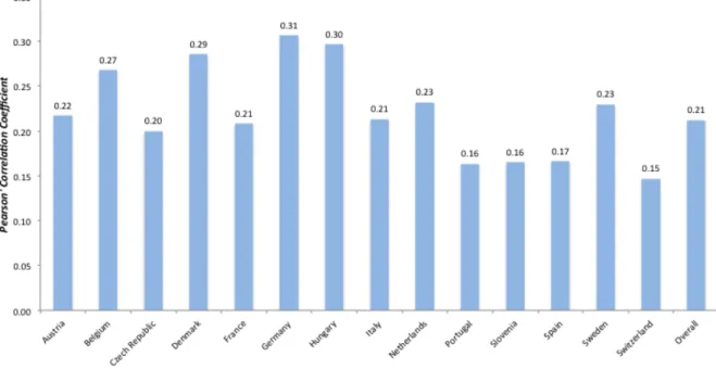
Figure 1 exhibits the average level of health for each country and for the overall sample. Our results show that the countries with worst level of health are Hungary, Portugal and Spain; with Switzerland, The Netherlands and Denmark performing better. The highest health discrepancies we find between the countries analyzed arise from Switzerland and Hungary, with a gap of 8.52 points in the level of health. Nevertheless, both countries exhibit a similar deviation in absolute value from the overall mean (- 4.20 for Hungary and 4.32 for Switzerland). Figure 2 represents Pearson’s Correlation Coefficients
between the severity-weighted index and total household wealth for each country and for the overall sample. Across all countries there is a positive correlation between the two variables, with the highest associations arising from Belgium, Denmark, Germany and Hungary; and the weakest from Portugal, Slovenia, Spain and Switzerland. The correlation for the overall sample (R=0.21) reveals a positive but moderately weak association between wealth and health.
Table 1 exhibits the main regression model predicting the severity-weighted index for each of the 14 countries in the sample. First, wealth shows a statistically significant effect on personal health, at a significance level of 1% for all the countries, except for Slovenia, where the significance level is 5%. Second, the impact of wealth on personal health is positive, meaning that being higher in the distribution of wealth implies better health. The impulse of the change in wealth is also relevant, as the impact of the coefficients varies, on average, from 0.017 in Slovenia to 0.092 in Germany; hence, a change in wealth from the 20th to the 80th percentile would yield an average impact on the health of an individual by 1.02 in Slovenia to 5.52 in Germany. Third, these results reinforce our hypothesis that wealth is likely to affect the level of health, and that the magnitude of this effect is likely to vary across countries. Finally, it is relevant to state that the coefficients for income happen to be statistically insignificant in Austria, Czech Republic, Italy, Spain and Switzerland, after controlling for wealth and socio-demographic characteristics. Also, in Portugal the income coefficient exerts a negative effect on health with 1% statistical significance. These findings could be interpreted as these countries’ healthcare systems trend to be efficient in either neutralizing or decreasing the health inequities associated with the level of household income.
Table 2 presents the estimates for five multiple regression models: the first is a replication of the model on Table 1 comprising the 14 countries in the sample, while in the other four models we add the estimation of the effects of GDP and current health expenditure per capita growth on health and on the magnitude of the wealth-based health inequalities. To estimate the regression models on Table 2, we first performed a Chow-test under the null hypothesis that all the coefficients of the 14 groups of countries were equal. Since the null hypothesis for the Chow-test was rejected, we have maintained only the variables that could hold on the usual 5% significance level and introduced the country-level indicators used on the models of Table 2. The magnitude and the statistical significance of the model’s coefficients had small changes. The only relevant change was for wealth, which lost statistical significance; however, the magnitude of the coefficient did not change substantially. Since the bias of the estimates happens to be minimal, we decided to proceed with the estimation of a single model comprising all countries in the sample. Model (1) confirms the overall results from Table 1: wealth exerts a statistically significant and positive effect on the level of health, after controlling for income, age, educational level, and immigration and partnership status. On the socio demographic side of this analysis, we find that age is contributing negatively to health, while being male and living with a partner are likely to increase the quality of health. Individuals with a low level of education are likely to have worse health than those with an intermediary or higher level of education. Finally, immigration status is not likely to have a statistically significant impact on individual health. Model (2a) estimates that a 1-percentage point increase in GDP per capita is likely to positively affect health (1.419). In model (2b), an interaction term of wealth with GDP was added, to understand what would be the effect of economic growth on
the relationship between wealth and health. This interaction was not statistically significant at the usual 5% level, and so we can conclude that this result is not relevant, despite the interaction term showing that richer countries tend to exhibit a lower magnitude on the wealth-health gradient. Model (2b) reiterates the results from model (2a) that countries with a higher level of economic resources are likely to have a better health status. Model (3a) repeats the previous analysis for current health expenditure. For instance, an annual increase of 1,000 € on current health expenditure per capita is likely to produce, on average, a positive impact of 2 units on self-assessed health. The interaction term introduced in model (3b) between total household wealth and current health expenditure proved to be statistically significant, and to negatively affect the health inequalities arising from wealth. The significance level of this interaction served as an incentive to perform the same analysis with current health expenditure from the general government and private sector.
In Table 3, it was estimated the impact of a 1-Euro per capita increase in out-of-pocket payments by private households, general government and private sector health expenditure on the severity-weighted index and on the wealth-health gradient. First, we find statistical significance on wealth for all the model estimations at the 1% significance level, controlling for socio economic and demographic attributes and for country-level variables. Second, the estimates point that an increase in health expenditures is likely to improve the quality of health. Third, all the interactions of the three components of health expenditure with wealth yield a statistically significant and negative effect on the magnitude of the health gap in models (1b), (2b) and (3b).
Given the statistical significance of the expenditure interactions with wealth in the models of Table 3, it was graphically estimated on Figure 3 the marginal impact of an
isolated 500-Euro increase in out-of-pocket, public and private health expenditures on the severity-weighted index, accounting for the distribution of wealth (first order derivatives in models (1b), (2b) and (3b) with respect to GHE, PHE and OPE, respectively). First, the graph reveals that a 500-Euro per capita increase in the private sector health expenditure is likely to exert, on average, a higher contribution to the level of personal health than an equivalent increase of public health or current health expenditure. Also, the same 500-Euro increase seems to produce an effect with a wider variability in the incremental benefits accounting for household wealth, due to the steepness of the line. By comparing both the increment of the private expenditure with the increment of public health expenditure, we see that the gap between them narrows as wealth increases, meaning that the benefits arising from the private health expenditure are more “wealth sensitive”. Second, we find the effect of both private sector and out-of-pocket health expenditure per capita to be producing very similar health improvements, although the effect of the out-of-pocket payments seem to benefit slightly less those with lower wealth and slightly more the one’s with higher wealth. Third, despite the results showing that a 500-Euro change in the public and private components of health expenditure produce, in quantitative terms, similar increments to health, depending on the individual’s level of household wealth, the difference between the marginal impacts can still differ substantially. This third consideration is confirmed on Table 4, which exhibits the estimates for a hypothetical per capita increase of 500 Euros in health expenditure, with the estimation of 95% confidence intervals for the impacts and their discrimination as a function of the level of household wealth. From the estimation of confidence intervals in Table 4, we conclude that as the wealth percentiles increase, the effects of private and public health expenditure on the
severity-weighted index tend to be approximately similar, and so the additional health benefits are higher with an increase of the private health expenditure between the wealth percentiles 0 and 50.
Table 5 presents four model estimations for the impact of the Gini index and the S80/S20 ratio on health, with interaction terms with wealth, in order to understand what would be the impact of higher income inequality on health and on the wealth-health gradient. According to models (1a) and (1b), a higher income concentration would not have a statistically significant impact on health, neither with the interaction with wealth. For models (2a) and (2b), we have found statistical significance on the impact of the S80/S20 ratio on health (- 0.202), but when it is controlled for the interaction term with wealth the statistical significance does not hold. The objective of this test was to understand which type of income inequality was most likely to affect the level of health: higher inequality between the 20% richest and the 20% poorest or lower income dispersion in a country? Given that the results are not statistically relevant, we conclude that country-level income inequalities are not associated with an individual’s quality of health.
Section 5: Conclusions
The objective of this work was to infer if household wealth is likely to contribute to health inequalities. In a first stage, we tested this hypothesis through OLS regression analysis in each of the 14 countries of our sample. In a second stage, all countries were combined in a single regression to test the effect of wealth on health, and the impact of macroeconomic indicators, such as GDP, total current health expenditure and measures of income inequality on health and on the wealth-health gradient.
First, we found considerable health discrepancies among the countries in the sample and, despite representing several regions in Europe, the correlations between the estimated health measure and total household wealth found to be positive and similar in magnitude across countries.
Second, the OLS regressions by country confirmed the significance of the impact of wealth on health, showing different magnitudes across countries and confirming our first hypothesis. In this estimation, we also found countries where income is likely to have a negative or neutral effect on health, probably justified by the efficiency of the healthcare systems in addressing income-associated health inequities.
Third, our results found a significant association between wealth and health on a regression accounting for the complete sample. Further estimations were made including GDP per capita and total current health expenditure per capita, comprising out-of-pocket, public and private health expenditures per capita. The estimations revealed that countries with higher amounts of economic resources are likely to exhibit better health standards, although no effect was found concerning the impact the state of the economy could have on the wealth-health gradient. On the other hand, the countries’ expenditure on health is likely to decrease the magnitude of the wealth-health gradient, according with the results. This finding was evident on the estimation of the marginal impacts on health, showing the private sector health expenditure associated with a stronger contribution to personal health and a higher diversity of the impact across the distribution of wealth when comparing with the general government expenditure. Therefore, our second hypothesis can be partially confirmed, with the exception that we did not find that economic growth is likely to significantly affect the magnitude of the health inequalities associated with health.
Fourth, the inclusion of national indicators of income inequality – the Gini index and the S80/S20 disposable income quintile ratio – revealed to have no effect on health and on the magnitude of the wealth-health gradient, with the exception of the economic discrepancies between the most rich and the most poor, which revealed to negatively affect personal health. In the effect explained by the S80/S20 ratio, the main difference from Semyonov et al. (2013) is that this effect on individual health is statistically significant with our sample of countries, which does not comprise the United States. Our third and last hypothesis, to infer whether a higher concentration of income in each country or a wider gap between the rich and the poor is more likely to impact health, could not be verified due to the lack of association of these effects with health and wealth.
Finally, the findings of this study point to the possibility that reducing income inequalities will not affect the already established health inequalities associated with personal wealth; but also raise the discussion that private healthcare systems may be more efficient than public systems in producing healthcare, with emphasis to the segment of the population in a more fragile economic position. We believe that the wealth-health gradient and these hypotheses should be tested with other econometric methods, namely through panel data models, to understand if these findings are consistent over different periods and how much can they change overtime. Moreover, and since we found interesting the inclusion of country-level indicators, multi-level and fixed-effect models could also be important to understand the magnitudes of country-level effects, controlling also for socio economic and socio demographic individual attributes. In either case, the findings should always be interpreted within the context of
self-assessed health, as long as surveys of large dimension do not adopt clinical metrics to measure the individual’s real health condition.
Figure 1 – Mean Severity-Weighted Health Index, by country.
Figure 2 – Pearson Correlation Coefficients between the Severity-Weighted Health
Index and Total Household Wealth, by country.
Figure 3 – Marginal Impact on the Severity-Weighted Health Index of a 500-Euro
increase in Current, Private Sector, General Government and Out-of-Pocket Health Expenditure per capita.
Italy Netherlands Portugal Slovenia Spain Sweden Switzerland Wealth (%) 0.062 0.048 0.042 0.017 0.043 0.044 0.028 (0.007)** (0.007)** (0.011)** (0.008)* (0.008)** (0.008)** (0.005)** Income (%) -0.004 0.021 -0.026 0.056 0.004 0.020 0.006 (0.007) (0.008)** (0.010)** (0.007)** (0.008) (0.009)* (0.005) Age (centered) -0.537 -0.194 -0.380 -0.333 -0.527 -0.322 -0.239 (0.022)** (0.022)** (0.034)** (0.022)** (0.023)** (0.030)** (0.016)** Male 3.920 2.154 5.476 1.077 4.986 1.618 1.029 (0.361)** (0.346)** (0.570)** (0.396)** (0.431)** (0.429)** (0.258)** Low education -1.685 -0.123 -6.050 -2.397 -2.352 -0.031 -1.359 (0.382)** (0.452) (0.833)** (0.489)** (0.591)** (0.565) (0.393)** High education 0.994 0.739 -1.425 1.536 0.831 0.855 0.170 (0.534) (0.448) (0.853) (0.458)** (0.721) (0.526) (0.316) Immigrant 0.975 -1.802 3.064 1.025 1.377 -1.904 -1.624 (1.372) (0.897)* (1.292)* (0.568) (1.035) (0.773)* (0.388)** Living w/ partner 1.169 0.633 1.357 -1.617 0.440 0.583 0.164 (0.545)* (0.524) (0.814) (0.521)** (0.586) (0.625) (0.362) Constant 84.350 86.600 85.494 86.212 84.012 87.121 91.012 (0.655)** (0.677)** (1.238)** (0.631)** (0.879)** (0.773)** (0.402)** Log Likelihood -13,013.368 -9,277.682 -7,652.704 10,005.528 -13,005.582 -6,757.469 -12,085.752 R2 0.27 0.13 0.18 0.18 0.25 0.16 0.14 N 3,451 2,589 1,938 2,688 3,309 1,859 3,541
Note: * p<0.05; ** p<0.01; Omitted variables: Female = 0; Intermediate education = 0; Native-born = 0; Not living with a partner = 0.
Table 1
OLS regression coefficients (robust standard errors) predicting the Severity-Weighted Health Index, by country.
Austria Belgium Czech
Republic
Denmark France Germany Hungary
Wealth (%) 0.052 0.071 0.037 0.060 0.047 0.092 0.088 (0.006)** (0.006)** (0.005)** (0.007)** (0.005)** (0.011)** (0.009)** Income (%) -0.009 0.020 0.009 0.018 0.021 0.024 0.029 (0.006) (0.006)** (0.005) (0.009)* (0.006)** (0.012)* (0.009)** Age (centered) -0.355 -0.340 -0.483 -0.235 -0.367 -0.372 -0.329 (0.018)** (0.016)** (0.018)** (0.024)** (0.015)** (0.039)** (0.029)** Male 0.443 2.885 2.057 1.222 2.295 1.578 3.303 (0.300) (0.290)** (0.287)** (0.378)** (0.262)** (0.552)** (0.465)** Low education -2.011 -1.150 -2.826 -1.635 -0.007 -2.145 -4.282 (0.398)** (0.375)** (0.308)** (0.645)* (0.330) (0.986)* (0.623)** High education 1.243 0.428 1.197 1.113 1.316 0.897 2.208 (0.323)** (0.351) (0.390)** (0.381)** (0.326)** (0.580) (0.551)** Immigrant 0.287 -0.306 -4.149 -1.858 -1.112 0.508 1.129 (0.516) (0.521) (0.794)** (1.017) (0.456)* (0.809) (1.687) Living w. partner 1.740 0.022 0.753 -0.277 -0.063 -1.230 -1.099 (0.361)** (0.387) (0.372)* (0.545) (0.341) (0.733) (0.633) Constant 86.334 82.137 85.142 86.941 84.278 83.221 78.582 (0.449)** (0.483)** (0.441)** (0.606)** (0.454)** (0.827)** (0.727)** Log Likelihood -18,729.34 -18,768.448 -21,942.113 -7,693.009 -19,834.973 -5,319.787 -11,766.963 R2 0.17 0.20 0.23 0.19 0.21 0.19 0.20 N 5,013 5,010 5,807 2,170 5,383 1,424 2,981
Table 2
OLS regression coefficients (robust standard errors) predicting the Severity-Weighted Health Index with the effect of Gross Domestic Product (GDP) and Current Health Expenditure (CHE) per capita.
Models (1) (2a) (2b) (3a) (3b) Wealth (%) 0.051 0.051 0.261 0.052 0.082 (0.002)** (0.002)** (0.120)* (0.002)** (0.005)** Income (%) 0.009 0.009 0.009 0.011 0.011 (0.002)** (0.002)** (0.002)** (0.002)** (0.002)** Age (centered) -0.356 -0.356 -0.356 -0.363 -0.362 (0.006)** (0.006)** (0.006)** (0.006)** (0.006)** Male 2.357 2.363 2.364 2.375 2.374 (0.098)** (0.098)** (0.098)** (0.097)** (0.097)** Low education -2.246 -2.191 -2.191 -1.656 -1.640 (0.116)** (0.116)** (0.116)** (0.116)** (0.116)** High education 0.859 0.918 0.915 0.795 0.817 (0.115)** (0.115)** (0.115)** (0.114)** (0.114)** Immigrant -0.156 -0.180 -0.186 -0.933 -0.968 (0.184) (0.184) (0.184) (0.184)** (0.184)** Living w/ partner 0.533 0.555 0.559 0.534 0.539 (0.132)** (0.132)** (0.132)** (0.131)** (0.131)** LnGDP - 1.419 2.454 - - (0.327)** (0.746)** Wealth*LnGDP - - -0.021 - - (0.012) CHE - - - 0.002 0.002 (0.000)** (0.000)** Wealth*CHE - - - - -0.000 (0.000)** Constant 85.056 70.470 59.866 79.841 78.281 (0.158)** (3.367)** (7.651)** (0.224)** (0.374)** Log Likelihood -178,179.27 -178,169.73 -178,168.01 -177,601.47 -177,581.77 R2 0.18 0.18 0.18 0.20 0.20 N 47,163 47,163 47,163 47,163 47,163
Table 3
OLS regression coefficients (robust standard errors) predicting the Severity-Weighted Health Index with the effect of General Government Health Expenditure (GHE), Private Sector Health Expenditure (PHE) and Private Households Out-of-pocket Expenditure (OPE).
Models
(1a) (1b) (2a) (2b) (3a) (3b)
Wealth (%) 0.052 0.082 0.051 0.068 0.051 0.061 (0.002)** (0.006)** (0.002)** (0.004)** (0.002)** (0.003)** Income (%) 0.011 0.011 0.010 0.010 0.010 0.010 (0.002)** (0.002)** (0.002)** (0.002)** (0.002)** (0.002)** Age (centered) -0.364 -0.363 -0.359 -0.358 -0.358 -0.358 (0.006)** (0.006)** (0.006)** (0.006)** (0.006)** (0.006)** Male 2.377 2.376 2.365 2.365 2.358 2.358 (0.097)** (0.097)** (0.097)** (0.097)** (0.097)** (0.097)** Low education -1.718 -1.702 -1.852 -1.842 -2.002 -1.997 (0.115)** (0.115)** (0.117)** (0.117)** (0.117)** (0.117)** High education 0.660 0.685 1.001 1.010 0.947 0.947 (0.114)** (0.114)** (0.115)** (0.115)** (0.115)** (0.115)** Immigrant -0.822 -0.853 -0.716 -0.739 -0.478 -0.491 (0.184)** (0.184)** (0.185)** (0.184)** (0.184)** (0.184)** Partner 0.546 0.555 0.517 0.514 0.506 0.504 (0.131)** (0.131)** (0.132)** (0.132)** (0.132)** (0.132)** GHE 0.003 0.003 - - - - (0.000)** (0.000)** Wealth*GHE - -0.000 - - - - (0.000)** PHE - - 0.003 0.005 - - (0.000)** (0.000)** Wealth*PHE - - - -0.000 - - (0.000)** OPE - - - - 0.003 0.005 (0.000)** (0.000)** Wealth*OPE - - - -0.000 (0.000)** Constant 79.504 77.952 82.720 81.881 83.381 82.875 (0.231)** (0.397)** (0.187)** (0.258)** (0.182)** (0.241)** Log Likelihood -177,551.37 -177,533.14 -177,938.09 -177,925.49 -178,023.79 -178,018.27 R2 0.20 0.20 0.19 0.19 0.19 0.19 N 47,163 47,163 47,163 47,163 47,163 47,163
Table 4
Estimation of the marginal impact on the Severity-Weighted Index of a 500-Euro increase in General Government and Private Sector Health Expenditure per capita, with 95% confidence intervals.
Wealth = 0 Wealth = 25 Wealth = 50 Wealth = 75 Wealth = 100 GHE 1.488 1.822 1.242 1.691 0.996 1.571 0.750 1.450 0.503 1.329 PHE 2.047 2.603 1.617 2.388 1.187 2.173 0.757 1.958 0.327 1.743
Table 5
OLS regression coefficients (robust standard errors) predicting the Severity-Weighted Health Index with the effect of the Gini Index and the S80/S20 disposable income quintile share ratio.
Models (1a) (1b) (2a) (2b) Wealth (%) 0.051 0.051 0.051 0.049 (0.002)** (0.018)** (0.002)** (0.010)** Income (%) 0.009 0.009 0.009 0.009 (0.002)** (0.002)** (0.002)** (0.002)** Age (centered) -0.356 -0.356 -0.356 -0.356 (0.006)** (0.006)** (0.006)** (0.006)** Male 2.360 2.360 2.365 2.365 (0.098)** (0.098)** (0.098)** (0.098)** Low education -2.214 -2.214 -2.142 -2.142 (0.118)** (0.118)** (0.119)** (0.119)** High education 0.864 0.864 0.871 0.872 (0.115)** (0.115)** (0.115)** (0.115)** Immigrant -0.161 -0.161 -0.181 -0.181 (0.184) (0.184) (0.184) (0.184)
Living with partner 0.539 0.539 0.550 0.551
(0.132)** (0.132)** (0.132)** (0.132)** Gini -0.021 -0.021 - - (0.018) (0.041) Wealth*Gini - 0.000 - - (0.001) S80/S20 - - -0.202 -0.221 (0.066)** (0.144) Wealth*S80/S20 - - - 0.000 (0.002) Constant 85.633 85.637 85.882 85.963 (0.532)** (1.160)** (0.315)** (0.645)** Log Likelihood -178,178.53 -178,178.53 -178,173.57 -178,173.56 R2 0.18 0.18 0.18 0.18 N 47,163 47,163 47,163 47,163
References
Beraldo, S., Montolio, D., Turati, G. 2009. “Healthy, educated and wealthy: A primer on the impact of public and private welfare expenditures on economic growth.” The Journal of Socio-Economics, 38: 946-956.
Börsch-Supan A., M. Brandt , H. Litwin and G. Weber (Eds). 2013a. Active ageing and solidarity between generations in Europe: First results from SHARE after the economic crisis. Berlin: De Gruyter.
Börsch-Supan, A., Brandt, M., Hunkler, C., Kneip, T., Korbmacher, J., Malter, F., Schaan, B., Stuck, S., Zuber, S. 2013b. Data Resource Profile: The Survey of Health, Ageing and Retirement in Europe (SHARE). International Journal of Epidemiology DOI: 10.1093/ije/dyt088.
Dahl, E., Birkelund, G. E. 1997. “Health inequalities in later life in a social democratic welfare state.” Social Science and Medicine, 44 (6): 871-881.
Demakakos, P., Nazroo, J., Breeze, E., Marmot, M. 2008. “Socioeconomic status and health: The role of subjective social status.” Social Science and Medicine, 67: 330-340.
Eikemo, T., Bambra, C., Judge, K., Ringdal, K. 2008a. “Welfare state regimes and differences in self-perceived health in Europe: A multilevel analysis.” Social Science and Medicine, 66: 2281-2295.
Eikemo, T., Bambra, C., Joyce, K., Dahl, E. 2008b. “Welfare state regimes and income-related health inequalities: a comparison of 23 European countries.” European Journal of Public Health, 18 (6): 593-599.
Fujishiro, K., Xu, J., Gong, F. 2010. “What does “occupation” represent as an indicator of socioeconomic status?: Exploring occupational prestige and health.” Social Science and Medicine, 71: 2100-2107.
Hurrelmann, K., Rathmann, K., Richter, M. 2010. “Health inequalities and welfare state regimes: a research note.” Journal of Public Health, 19: 3-13.
Malter, F., Börsch-Supan, A.(Eds.) 2013. SHARE Wave 4: Innovations & Methodology. Munich: MEA, Max Planck Institute for Social Law and Social Policy.
Maskileyson, D. 2014. “Healthcare system and the wealth-health gradient: A comparative study of older populations in six countries.” Social Science and Medicine, 119: 18-26.
Meer, J., Miller, D., Rosen, H. 2003. “Exploring the wealth-health nexus.” Journal of Health Economics, 22: 713-730.
Morris, J. N., Donkin, A. J. M., Wonderling, D., Wilkinson, P., Dowler, E. A. 2000. “A minimum income for healthy living.” Journal of Epidemiology and Community Health, 54: 885-889.
Pampel, Fred C., Krueger, Patrick M., Denney, Justin T. 2010. “Socioeconomic Disparities in Health Behaviors.” Annual Review of Sociology, 36: 349-370.
Pickett, K., Wilkinson, R. 2015. “Income inequality and health: A causal review.” Social Science and Medicine, 128: 316-326.
Qin, X., Hsieh, C. 2014. “Economic growth and the geographic maldistribution of health care resources: Evidence from China, 1949-2010.” China Economic Review, 31: 228-246.
Rutstein, Shea O., Johnson, K. 2004. “The DHS Wealth Index.” DHS Comparative Reports, 6: 4.
Schnittker, J., Bacak, V. 2014. “The Increasing Predictive Validity of Self-Rated Health.” PLoS ONE, 9 (1): e84933.
Semyonov, M., Lewin-Epstein, N., Maskileyson, D. 2013. “Where wealth matters more for health: The wealth-health gradient in 16 countries.” Social Science and Medicine, 81: 10-17.
Van Doorslaer, E., Wagstaff, A., Bleichrodt, H., Calonge, S., Gerdtham, U., Gerfin, M., Geurts, J., Gross, L., Häkkinen, U., Leu, R., O’Donnell, O., Propper, C., Puffer, F., Rodríguez, M., Sundberg, G., Winkelhake, O. 1997. “Income-related inequalities in health: some international comparisons.” Journal of Health Economics, 16: 93-112.
Van Kippersluis, H., Galama, Titus J. 2014. “Wealth and health behavior: Testing the concept of a health cost.” European Economic Review, 72: 197-220.
Veugelers, P. J., Yip, A. M. 2003. “Socioeconomic disparities in health care use: Does universal coverage reduce inequalities in health?” Journal of Epidemiology and Community Health, 57: 424-428.
Wang, K. 2011. “Health care expenditure and economic growth: Quantile panel-type analysis.” Economic Modelling, 28: 1536-1549.
Wu, S., Wang, R., Zhao, Y., Ma, X., Wu, M., Yan, X., He, J. 2013. “The relationship between self-rated health and objective health status: a population based study.” BMC Public Health, 13: 320.
Appendix 1
Data source, year of data collection and sample size, by country
Country Data source Year of data collection Wave observations Number of
Austria SHARE 2011 4 5,013
Belgium SHARE 2011 4 5,010
Czech Republic SHARE 2011 4 5,807
Denmark SHARE 2011 4 2,170 France SHARE 2011 4 5,383 Germany SHARE 2011 4 1,424 Hungary SHARE 2011 4 2,981 Italy SHARE 2011 4 3,451 Netherlands SHARE 2011 4 2,589 Portugal SHARE 2011 4 1,938 Slovenia SHARE 2011 4 2,688 Spain SHARE 2011 4 3,309 Sweden SHARE 2011 4 1,859 Switzerland SHARE 2011 4 3,541 Total - - - 47,163
Appendix 2
Mean Severity-Weights (standard-deviation) for the 41 health problems.
Health Problems Mean Severity Std. D.
Difficulty dressing, including shoes and socks 6.62 (1.73)
Difficulty walking across a room 7.00 (1.92)
Difficulty bathing or showering 6.62 (1.21)
Difficulty eating, cutting up food 5.46 (2.13)
Difficulty getting in or out of bed 6.77 (1.76)
Difficulty using the toilet, including getting up or down 7.54 (2.02)
Difficulty walking 100 meters 5.85 (1.70)
Difficulty sitting two hours 4.69 (1.73)
Difficulty getting up from chair 5.38 (2.10)
Difficulty climbing several flights of stairs 4.62 (1.73)
Difficulty climbing one flight of stairs 6.08 (2.13)
Difficulty stooping, kneeling, crouching 4.85 (1.92)
Difficulty reaching or extending arms above shoulder 4.77 (1.93)
Difficulty pulling or pushing large objects 3.77 (1.58)
Difficulty lifting or carrying weights over 5 kilos 4.08 (2.20)
Difficulty picking up a small coin from a table 4.69 (2.30)
Heart attack 8.38 (1.21)
High blood pressure or hypertension 6.31 (2.55)
High blood cholesterol 5.62 (2.37)
Stroke 9.08 (0.83)
Diabetes or high blood sugar 6.92 (1.73)
Chronic lung disease 7.08 (1.73)
Asthma 6.31 (1.59)
Arthritis 6.69 (1.64)
Osteoporosis 5.92 (2.37)
Cancer 8.54 (1.78)
Stomach or duodenal ulcer, peptic ulcer 5.85 (1.56)
Parkinson disease 8.23 (1.67)
Cataracts 6.46 (1.08)
Hip fracture or femoral fracture 8.54 (1.95)
Pain in back, knees, hips or other joint 5.46 (1.95)
Heart trouble 7.00 (1.41) Breathlessness 7.46 (1.39) Persistent cough 5.92 (1.38) Swollen legs 5.31 (1.49) Sleeping problems 5.77 (1.37) Falling down 7.00 (2.11)
Fear of falling down 5.69 (2.23)
Dizziness, faints or blackouts 7.08 (1.90)
Stomach or intestine problems 5.69 (1.90)
Appendix 3 (I)
Independent variables definition and descriptive statistics.
Variable name Variable definition Mean (SD) or percentage
Wealth Total household wealth, comprising all net real and
net financial assets, minus debt 241,866.5 (661,751.7) Income Total household income, comprising all non-asset
income
32,727.2 (47,390.34)
Age In years and centered around its mean 66.20 (10.04)
Gender Male (=1) 44.52
Female (=0) 55.48
Education High (=1) – Tertiary education 20.45
Intermediate (=0) – Upper secondary or post-secondary (non-tertiary) education
36.69 Low (=1) – Lower secondary, primary or no
education
42.86
Immigrant Immigrant (=1) 7.27
Native-born (=0) 92.73
Living with partner Living with partner (=1) 72.30
Single (=0) 27.70
GDP Annual Gross Domestic Product per capita 28,534.15 (4544.35)
CHE Annual total current health expenditure per capita 2,692.30 (926.48) GHE Annual current general government health
expenditure per capita
2,056.29 (683.57) PHE Annual current private sector health expenditure per
capita
636.00 (326.29) OPE Annual private households out-of-pocket health
expenditure per capita
447.77 (251.11) Gini Gini index, at disposable income, post taxes and
transfers
28.61 (2.90) S80/S20 S80/S20 disposable income quintile share ratio 4.48 (0.85) Note: Wealth, Income, GDP, CHE, GHE, PHE and OPE were adjusted for PPP and converted into Euros.
Appendix 3 (II)
Descriptive statistics, by independent variable and country. Austria Belgium Czech
Republic Denmark France Germany Hungary Wealth 169,864.5 (263,188.1) 330,121.8 (391,019.6) 116,801.2 (125,756.2) 249,518.3 (324,527.1) 289,421 (542,93) 199640 (252,100.9) 145,970.4 (1,983,06) Income 29,589.89 (26,425.72) 52,413 (68,533.5) 17,073.54 (15,326.16) 30,554.96 (18,956.84) 31,966.05 (47,169.85) 29,756.25 (23,793.25) 11,662.93 (10,400.09) Age 66.01 (9.79) 65.47 (10.64) 65.57 (9.44) 65.05 (10.53) 66.35 (10.75) 68.47 (8.73) 65.12 (9.38) Male 42.67 45.33 42.90 46.36 44.03 46.70 43.84 High Education 25.29 30.38 12.31 41.71 20.17 30.34 15.97 Low Education 25.07 43.13 45.62 18.39 46.00 13.27 31.83 Immigrant 8.58 9.30 4.70 3.09 10.37 13.00 1.95 Living w/ partner 64.91 69.10 70.17 74.19 67.73 78.93 71.79 GDP 30,681.54 27,558.77 38,391.36 21,909.28 25,974.78 29,386.36 26,051.92 CHE 30,681.54 3,068.42 1,804.91 2,963.57 3,059.55 3,133.82 1,038.81 GHE 2,539.47 2,321.96 1,514.02 2,511.49 2,378.28 2,412.69 656.46 PHE 745.12 746.46 290.90 452.08 681.27 721.14 382.35 OPE 554.34 612.13 271.12 394.37 238.61 386.06 290.33 Gini 28.18 26.43 25.61 25.27 30.9 29.31 27.19 S80/S20 4.4 4 3.7 3.6 4.7 4.4 4
Note: Wealth, Income, GDP, CHE, GHE, PHE and OPE were adjusted for PPP and converted into Euros; standard deviations inside brackets; age, male, education level, immigrant and partnership status are expressed in percentage.
Appendix 3 (III)
Descriptive statistics, by independent variable and country.
Italy Netherlands Portugal Slovenia Spain Sweden Switzerland Wealth 234,219.5 (331,851.4) 257,439.4 (514,434.3) 169,232.2 (294,829.8) 192,858.6 (222,433.2) 270,821.4 (547,204.6) 253,933.1 (331,147.6) 484,389.2 (895,148.5) Income 23,953.34 (31,138.98) (32,133.76) 39,211.44 (91,328.92) 23,063.69 (46,567.07) 34,764.15 (20,452.5) 19,765.75 (24,098.79) 33,771.39 (76,673.78) 75,519.73 Age 67.01 (9.55) 66.018 (9.58) 65.18 (9.50) 65.70 (10.01) 68.03 (10.80) 70.06 (9.02) 65.51 (10.06) Male 45.55 44.34 44.53 43.94 45.45 45.94 45.95 High Education 6.52 26.65 28.38 16.37 8.55 26.30 15.87 Low Education 70.88 47.32 64.55 34.78 82.02 45.99 20.05 Immigrant 1.30 5.06 3.25 10.75 2.78 8.77 17.17 Living w/ partner 79.83 76.98 78.79 73.55 77.18 71.17 75.12 GDP 24,282.36 32,748.99 22,412.55 26,784.98 25,598.98 26,552.9 29,929.7 CHE 2,068.84 3,679.30 1,686.6 1,867.07 2,102.32 2,910.22 4,766.48 GHE 1,638.17 3,152.68 1,105.09 1,368.87 1,540.84 2,375.11 3,114.96 PHE 430.67 526.62 581.51 498.20 561.48 535.10 1,651.52 OPE 409.93 216.81 487.73 228.62 433.91 497.59 1,199.09 Gini 32.14 28.3 34.14 24.50 34.39 27.34 28.90 S80/S20 5.6 4.2 5.8 3.6 6.7 4.1 4.4
Note: Wealth, Income, GDP, CHE, GHE, PHE and OPE were adjusted for PPP and converted into Euros; standard deviations inside brackets; age, male, education level, immigrant and partnership status are expressed in percentage.
Appendix 4
2SLS regression coefficients (robust standard-errors) predicting the Severity-Weighted Health Index.
Wealth (%) 0.068 (0.003)** Income (%) 0.005 (0.002)* Age (centered) -0.357 (0.006)** Male 2.364 (0.098)** Low education -2.142 (0.117)** High education 0.718 (0.116)** Immigrant -0.016 (0.185)
Living with partner 0.365
(0.134)**
Constant 84.522
(0.174)**
R2 0.18
N 47,163