Animal Spirits vs
Contagion:
Which one is the main
driver of sovereign yields
in Europe?
Miguel Homem Ferreira
Luís Catela Nunes
José Tavares
Working Paper
# 604
* The views in this paper do not reflect those of the Portuguese Treasury and Debt Management Agency (IGCP).
Animal Spirits vs Contagion:
Which one is the main driver of sovereign yields in Europe?
*Miguel Homem Ferreira, Nova School of Business and Economics and IGCP Luís Catela Nunes, Nova School of Business and Economics
José Tavares, Nova School of Business and Economics and CEPR
July 7, 2016
Abstract
The objective of this paper is to assess the differences between contagion and investors’ risk aversion in terms of their impact on European sovereign bond yields during the financial crisis. This paper evaluates contagion at banking level, as it has the advantage of capturing the exposure of sovereign debt markets to financial sector’s risk and also the contagion between sovereign spreads that occurs through the financial sector channel. The paper analyzes the period from 2008 to 2012 and also the Greek, Portuguese and Spanish bailout periods. The results indicate that the main driver of yields in Europe is risk aversion and not contagion. The main differences between Central and Southern European countries’ yields are explained by risk aversion. This channel has a much stronger impact on the periphery. On the other hand, contagion exerts a similar influence throughout all European countries.
2
1. Introduction
The main objective of this paper is to assess the differences between contagion and investors’ risk aversion in terms of their impact on European sovereign bond yields during the financial crisis. In the literature both variables are often confused, with risk aversion perceived as contagion and the other way around. In this paper the difference between contagion and risk aversion will be clarified, with the conclusion that the different behaviors of sovereign yields between Southern and Central European countries during the current crisis were caused mainly by investors’ risk aversion and not contagion.
This study will also evaluate the contagion and risk aversion during the two Greek bailouts as well as the debt restructure and the Spanish and Portuguese bailouts. That will help to understand if the increase in Southern European countries’ yields during these events was triggered by contagion or risk aversion. Once again, it will be possible to conclude that the difference between the core and European peripheral countries occurs due to risk aversion and not contagion, as the contagion affects all countries in the same way.
The paper will evaluate contagion from banks to countries. As discussed in the literature, the banking sector risk is connected to the country’s risk. Nonetheless, there is no quantification of the contagion of banking risk in one country to another country’s risk. With the methodology used in this paper it will be possible to quantify the contagion from a bank in country A to a bank in country B and then display how it affects country’s B sovereign bond yields.
Since the introduction of the Euro two different phenomena regarding the behavior of the sovereign interest rates of the European Monetary Union (EMU) countries could be observed. From 1999 until the start of the financial crisis in 2008, the sovereign bond interest rates converged, with spreads very close to zero. After 2008, there has been a divergence between Southern and Central Euro Area sovereign bond yields, with Germany often mentioned as a "safe heaven".
In 1999 there were significant differences in interest rates between peripheral countries (like Portugal, Greece or Italy) and core countries (France or Germany) with country specific factors, such as economic growth, budget deficits, level of debt, playing an important role. However, with the introduction of the Euro, country specific risks started to lose their significance within the EMU countries, and interest rate differentials almost disappeared. Pozzi and Wolswijk (2008) studied the period between 1995 and 2006 and concluded that by 2006, in the EMU, country specific factors did not play an important role.
Bernoth and Erdogan (2010) pointed out that with the formation of the EMU some factors, such as debt and deficits of the issuing country, did not have as much impact on sovereign spreads when compared with the period before the establishing of the EMU. Bernoth, von Hagen and Schuknecht (2006) also show that with the establishment of the EMU there was a change of focus on the fundamental macroeconomic variables of each country, from debt and deficits to debt service ratio.
Codogno, Favero and Missale (2003) highlighted some differences on the determinants of yield spreads before and after the EMU. Before the EMU, expected exchange rate movements, tax treatments, control on capital movements, liquidity and credit risk were the main factors affecting yield spreads within future EMU countries. However, in 1999, in spite of the introduction of the Euro, exchange rate related risks vanished in EMU countries. Also, control of the capital movements and different tax treatments were harmonized before the EMU. Consequently, the two factors that remained relevant were liquidity and default risk, indicating that Euro government bonds were not perfect substitutes.
3
Buiter and Grafe (2003) also shared this point of view, arguing that they found the convergence of the interest rates a surprising fact considering that the adoption of a single currency does not eliminate sovereign default risk differentials. They proved that even though interest rates (both long and short term) were converging, the short term real interest rates were not converging.
Although the sovereign interest rates were converging, there were still minor differences between the EMU countries. Pagano (2004) pointed out that liquidity, default risk and vulnerability to the risk of an eventual EMU collapse were the cause of the minor spread differentials in the beginning of the EMU. In addition to those factors, Heppke-Falk and Hufner (2004) mention the expectations built about the future country's deficit. Nevertheless there is some discrepancy in the impact of the expected deficits. While Canzoreni et al. (2002) proved that expected deficits would affect both long and short term sovereign interest rates, Laubach (2003,2004) and Gale and Orszag (2004) proved only a relation with long term interest rates. Ardagna, Carelli and Lane (2004) also demonstrated that deficits affected long term interest rates and that there was a non-linear relation between the level of government debt and sovereign bond yields: only when the debt ratio is above a certain threshold, does it affect sovereign yields.
Baek, Bandopadhyaya and Du (2005) argued that the market premium of country risk is affected by liquidity, solvency, economic stability and investor's attitude towards risk. Nonetheless the market premium could be affected in different ways depending if it is on long or short term maturities. According to Eichler and Maltritz (2012) indicators such as the growth rate of debt and trade balance affected more long term maturities whereas GDP growth rate and openness (proxied by exports plus imports) impacted all the maturities.
Meanwhile, with the eruption of the financial crisis in 2008, EMU sovereign bond yields started to diverge and investors became more risk averse and focused more on country specific fundamentals, like debt and deficit levels. Dötz and Fischer (2010) claim that the turning point from a non-crisis period to a crisis period was the bailout of Bear Stearns in 2008. They estimate a pre- crisis and a crisis specification to find out two major differences. On the pre-crisis period spreads for corporate bonds and the real exchange rate had a negative impact on sovereign bond yield spreads, whereas on the crisis periods both variables had a positive and statistically significant impact.
After 2008, the differentials were caused mainly by an overall increase in risk aversion, contagion and an increase in the price of risk (Bernoth and Erdogan, 2010). Investors behavior during crisis periods had been previously studied by Dungey et al (2000), Copeland and Jones (2001) and Lemmen (1999), all agreeing that during a crisis period there was a tendency among investors to move to safer and more liquid assets, further widening the spreads. Moreover, the findings of Sgherri and Zoli (2009) are in line with that perception, given that their finding that after the beginning of the financial crisis, the liquidity of markets had a major impact on sovereign bonds, explained by the "flight to safety" by investors. Gomez-Puiz (2006) and Manganelli and Wolswijk (2009) also argued that differentials in spreads were explained by liquidity. According to Mody (2009), investors paid more attention to the weaknesses of financial markets and determinants of country's specific risk.
Equally, Abmann and Boysen-Hogrefe (2009) show that there were major differences on how sovereign spreads were affected between 2003 and 2007 and after 2007. Between 2003 and 2007 debt to GDP ratio was the most important ratio for investors. That was not the case after 2007 when budget balances and liquidity started to play a much more important role. Since liquidity started to have a bigger impact on sovereign bond yield spreads, banking risk also affected the spreads through three main factors: shortage in banking liquidity, government recapitalization of banks, and bank
4
bailouts. Ejsing and Lemke (2010) also found a positive correlation between sovereign and banks CDS premia, strengthening the idea that banking risk had an impact on country risk.
Contagion also ignited the divergences between Euro countries’ sovereign bond yields. Arghyrov and Kontonikas (2012) provided a specification to evaluate how contagion affected spreads. They divided the EMU countries into two groups: the core and the periphery. They saw how each country was affected by the average of spreads of EU countries and how periphery countries and core countries affected the spreads. That enabled them to conclude that there was intra periphery contagion, i.e. between countries of the periphery group, and periphery to core contagion, with Greece, Ireland, Portugal and Spain being the main drivers of contagion.
Even though that literature significantly expands the knowledge on the determinants of sovereign bond yield spreads, there are still some gaps regarding the evaluation of the impact of contagion and investors’ risk aversion as well as the study of how certain events taking place in a given country spread out to other countries. This is where this paper will contribute to the literature, by estimating the impact of banking contagions and differentiating it from risk aversion, both during the crisis period and the bailout events in the given countries.
The paper is organized as follows. In Section 2 the model and the variables of interest are presented. In sections 3 and 4 the results of the model during the entire period considered and during the sovereign bailouts are displayed, while in Section 5 the overall results of the study are discussed. Section 6 present some robustness tests and Section 7 concludes the paper.
2. Instruments estimation
A change in sovereign interest rates is usually associated with changes in country’s specific fundamentals such as debt to GDP ratio, GDP growth rate, government deficits. However the phenomenon of sovereign interest rates fluctuations may also be due explained by other reasons. This paper will focus on the effects of contagion and changes in risk averseness among investors.
At times, countries that were not experiencing any macroeconomic changes have watched their sovereign bond yield spreads changing. This may occur as a result of contagion. As the current Eurozone countries have strong economic links, with free capital movements between countries, a common currency, among other reasons, a change in one country’s specific fundamentals will affect not only the sovereign bond yields of this particular country but also the yields for other countries.
Furthermore, the sovereign interest rates may change due to risk aversion of investors. The price of an asset is usually modeled on its returns and on the risk premium required by investors to buy that asset. As investors become more risk averse they will demand higher risk premiums, which leads to an increase in sovereign spreads.
To capture these two effects, this paper will use an approach adopted by Caceres, Guzzo and Segoviano (2010). Two variables, the Spillover Coefficient (SC) and the Index of Risk Aversion (IRA), will be constructed. The first variable will allow us to quantify the impact of banking contagion, by measuring the probability of default of a bank in a country i conditional on the fact that the bank in a country j defaults, while the second one will capture the investors’ risk aversion by measuring the required price of risk.
5 Spillover Coefficient (SC)
To estimate the Spillover Coefficient a bank’s default probability will be extracted from CDS data. It will be then used to calculate how it may impact another bank’s default probability. This way it is possible to quantify how changes on one bank’s risk affects another bank’s distress probability.
The SC variable will be calculated as the probability of bank in country i defaulting given that a bank in country j defaults, weighted by the probability of the bank in country j defaulting. SC is then given by
𝑆𝐶𝑖𝑡 = 𝑃(𝐴𝑖𝑡|𝐴𝑗𝑡) ∗ 𝑃(𝐴𝑗𝑡) ∀ 𝑗 ≠ 𝑖 where 𝑃(𝐴𝑗) is the probability of default of a bank in country j1, 𝑃(𝐴
𝑖|𝐴𝑗) is the probability of distress of bank in country i given that bank in country j defaults. To calculate the conditional probability of default 𝑃(𝐴𝑖𝑡|𝐴𝑗𝑡), the CIMDO method (Segoviano, 2006) will be used, thanks to which it will be possible to find the joint probability of default, 𝑃(𝐴𝑖𝑡, 𝐴𝑗𝑡), given that the joint probability will be necessary to find the conditional probability using Bayes’ Law
𝑃(𝐴𝑖𝑡|𝐴𝑗𝑡) =
𝑃(𝐴𝑖𝑡, 𝐴𝑗𝑡) 𝑃(𝐴𝑗𝑡) .
The CIMDO method consists in extracting from the data information on the unknown density probabilities (posterior distribution p(x,y) ). As the probabilities are extracted only from data of our interest there will be no need to recalibrate the probabilities since they will be consistent with the empirical data.
By creating a prior distribution (q(x,y)) in accordance with economic intuition and theoretical models we are able to model a problem to minimize the differences between the prior and the posterior distribution. By constructing an objective function of the form
𝐶[𝑝, 𝑞] = ∫ ∫ 𝑝(𝑥, 𝑦)𝑙𝑛 [𝑝(𝑥, 𝑦)
𝑞(𝑥, 𝑦)] 𝑑𝑥 𝑑𝑦 with a set of constraints given by
∫ ∫ 𝑝(𝑥, 𝑦)𝕀[𝑋 𝑑𝑥,∞)𝑑𝑥 𝑑𝑦 = 𝑃𝑜𝐷𝑡 𝑥 ∫ ∫ 𝑝(𝑥, 𝑦)𝕀[𝑋 𝑑 𝑦 ,∞)𝑑𝑦 𝑑𝑥 = 𝑃𝑜𝐷𝑡 𝑦 𝑝(𝑥, 𝑦) ≥ 0 ∫ ∫ 𝑝(𝑥, 𝑦)𝑑𝑥 𝑑𝑦 = 1
where 𝑃𝑜𝐷𝑡𝑖 is the probability of default of bank i at time t. This way it is possible to achieve the posterior distribution that is closest to the prior distribution but still consistent with empirical
1 Probability of default of country j is calculated using the Credit Default Swaps of this country and using a recovery rate
6
observations. At a next stage the joint probability of default, C[p,q], is obtained by replacing the prior and posterior distributions on the objective function. 2
Index of Risk Aversion (IRA)
The IRA is an index that reflects the market perception of risk in each period, which in turn leads to changes in investors’ risk aversion. It quantifies the perception of risk among investors as it incorporates the volatility of the market and the distress probability perceived by investors. With this the price of risk asked by investors is calculated. The higher the price of risk the higher the investors’ risk aversion with respect to that asset.
The IRA is given by
𝐼𝑅𝐴𝑖𝑡 = −(1 − 𝑃𝑜𝑅𝑖𝑡) = − (1 −𝑉𝑜𝑙𝑎𝑡𝑖𝑙𝑖𝑡𝑦 𝑜𝑓 𝑚𝑖𝑡
𝜋𝑖𝑡 )
where 𝑃𝑜𝑅𝑖𝑡 stands for Price of Risk, 𝜋𝑖𝑡 is the actual probability of default and 𝑚𝑖𝑡 is the price of security i. The volatility of 𝑚𝑖𝑡 will be equal to the market price of risk, which will be extracted from the Volatility Index VIX (measures the implied volatility of the S&P500) as proposed by Espinoza and Segoviano (2011). The actual probability of default will be estimated following a methodology suggested by Espinoza and Segoviano (2011)3. It will be given by
𝜋𝑡 =
𝜋𝑡 ̂
(1 + 𝑟𝑡𝑓)𝐸𝑡(𝑚𝑡+1|𝑑𝑖𝑠𝑡𝑟𝑒𝑠𝑠) using the risk neutral probability 𝜋̂ that can be calculated as 𝑡
𝜋𝑡
̂ = 𝑆𝑁
(1 − 𝐾)
with 𝑆𝑁 being the CDS spreads of country N and K the recovery rate, which we will assume equal to 60%. To estimate the market price of risk in a stress situation we will define distress as the price of risk above a certain threshold value, and assuming mt+1 is normally distributed it is possible to use the truncated normal distribution formula so that
𝐸𝑡(𝑚𝑡+1|𝑑𝑖𝑠𝑡𝑟𝑒𝑠𝑠) = 𝐸𝑡(𝑚𝑡+1|𝑚𝑡+1> 𝑇) = 𝜇𝑡+ 𝜎𝑡𝜆(α𝑡) with 𝜇𝑡= 𝐸[𝑚𝑡+1] 𝜎𝑡 = 𝑉𝑎𝑟(𝑚𝑡+1) 𝜆 = 𝜑(𝛼) [1 − Φ(α)] α𝑡= 𝑡ℎ𝑟𝑒𝑠ℎ𝑜𝑙𝑑 − 𝜇𝑡 𝜎𝑡
where Φ is the normal cumulative distribution function and 𝜑 is the normal density function. The threshold will be given by
2 See Annex I for detailed information of the CIMDO methodology. 3 See Annex II for calibration of the actual probability of default
7 𝑇 = 𝐸[𝑚] + Φ−1[1 − 𝜋 𝑡]√𝑣𝑎𝑟(𝑚) = 1 1 + 𝑟̅+ Φ −1[1 − 𝜋 𝑡]𝜎̅ so the actual probability of default will be given by the non-linear equation
𝜋𝑡 = 𝜋𝑡 ̂ 1 + (1 + 𝑟𝑡𝑓)𝜎𝑡∗ 𝜆 ( 1 1 + 𝑟̅ − 1 1 + 𝑟𝑡𝑓+ Φ −1[1 − 𝜋 𝑡]𝜎̅ 𝜎𝑡 ) . Methodology
With the two variables that account for contagions and risk aversion calculated, the baseline specification can now be estimated. Daily observations from 31st of May 2008 to 31st of December 2014 for all initial Eurozone countries except Luxembourg, Finland, Ireland and Netherlands due to the lack of CDS spreads data, will serve as the database for this very study. All the financial data is the last updated price data provided by Bloomberg while the country’s specific data comes from Eurostat.
From each country the bank that owns more debt of that country was selected to guarantee the connection between that bank and the sovereign yields. Nevertheless due to the lack of data of CDS spreads for some countries it was impossible to select in each case the bank that holds more national debt. The banks selected were Millennium BCP for Portugal, BBVA for Spain, Deutsche Bank for Germany, Intesa Sanpaolo for Italy, BNP Paribas for France, Erste Group Bank for Austria, KBC Bank for Belgium and Alpha Bank AE for Greece.
With the objective of measuring the impact of contagion and risk aversion on the sovereign yields, the following T-GARCH model will be used
Mean equation 𝑟𝑖𝑡 = 𝛽0+ 𝛽1(𝑟𝑖𝑡−1) + 𝛽2 𝑃𝑢𝑏𝑙𝑖𝑐 𝐷𝑒𝑏𝑡 𝐺𝐷𝑃 𝑖𝑡+ 𝛽3 𝐵𝑢𝑑𝑔𝑒𝑡 𝐷𝑒𝑓𝑖𝑐𝑖𝑡 𝐺𝐷𝑃 𝑖𝑡+ 𝛽4(𝐼𝑅𝐴𝐺𝐸𝑅𝑡) + ∑𝑗≠𝑖,𝑘𝛽𝑘𝑆𝐶𝑗𝑡+ 𝜀𝑖𝑡 Variance Equation 𝑉𝑎𝑟(𝜀𝑖𝑡|Ω𝑖𝑡−1) = 𝜎𝑖𝑡2 = 𝜔 + 𝜃𝜀𝑖𝑡−12 + 𝛾𝜎𝑖𝑡−12 + 𝛼𝜀𝑖𝑡−12 𝐼(𝜀𝑖𝑡−1 < 0)
where i stands for the country in study, j all the other countries in the sample and t the period. The dependent variable is the 5-year sovereign bond yield. A lag of the dependent variable is also included as an independent variable to control the high persistency of bond yields. Public debt and budget deficit as percentage of GDP are also incorporated in the specification as control variables for country fundamentals. The two main variables of interest are the German IRA and SC variables.
Only the German IRA was included, as it works as a good proxy for investors’ risk aversion with respect to Eurozone countries. This way it is easier to draw comparisons between the results in different countries. The SC variable will allow us to measure the impact of contagion between banks on the sovereign yields, and will serve as the contagion from foreign banks to the sovereign.
𝜀𝑡 is the error term with conditional variance given by a lag of the square of the error term itself (ARCH term), the conditional variance of the previous period (GARCH term) and also by a lag of the error term multiplied by an indicator function that will be equal to one if the error term is below zero, and zero otherwise (TARCH term).
8
The T-GARCH model was chosen to correct the heteroscedasticity present in the OLS equation. The addition of the TARCH term will account for the fact that variance may be asymmetrically dependent on the residuals.
3. Risk aversion vs banking contagion: Impact on sovereign yields
Contagion and investors risk aversion are often perceived as the same phenomenon. Some studies use both perceptions together to state that contagion is caused by an increase in investors’ risk aversion or the other way around. The results of this paper will distinguish the two phenomena and demonstrate that investors risk aversion plays more important role than pure contagion.
Baek, Bandophadyaya and Chan Du (2005) constructed a quantifiable measure of market's attitude towards risk that allows us to understand how countries that do not experience changes in economic indicators have spreads changing, to conclude that contagion was the main factor.
Another perspective of contagion is presented by Giordano, Pericoli and Tommasino (2013). Instead of just looking at contagion and its sources, they took a different approach defining three distinct processes of contagion. The first was “Wake-up call contagion” which occurs when a crisis taking place in a country makes investors more risk averse with respect to a country that was economically similar to the country dealing with the crisis.
The second type was “Shift contagion”. This process was characterized by contagion occurring due to the intensification of the normal market channels and higher focus on factors common to different countries. The final definition was “Pure contagion” regarded as contagion coming from investors’ rationality, loss of confidence or capital losses in the country where the crisis originated. Here the focus will be on contagion having its source in foreign banks and the isolation of this effect so that it is not confused with investors’ price of risk demanded. Morison and White (2013) demonstrated that contagion between banks within the Euro Area takes place as banks are exposed to the same regulations. They found that the common regulations and not the correlation of the assets or interbank lending served as the main cause of contagion. This can be explained in the following way: if one bank fails it will lead to the loss of public confidence in the regulations and hence in banks subject to the same regulations.
Abmann and Boysen-Hogrefe (2009) and Ejsing and Lemke (2011) emphasized the connection between banking risk and sovereign yields, proving that after the beginning of the financial crisis liquidity and consequently the banking sector, started playing a huge role in the definition of sovereign yields. Acharya, Drechsler and Schnabl (2013) also demonstrated the link between the bank and sovereign risk, arguing that financial sector bailouts contributed to the outbreak of the crisis and the increase of sovereign risk.
Stânga (2014) also found a connection between banking bailouts and sovereign risk in European countries.
Using this knowledge about contagion between banks and the linkage with sovereign risk, we are comfortable with our approach when calculating the SC variable and with its connection to sovereign yields.
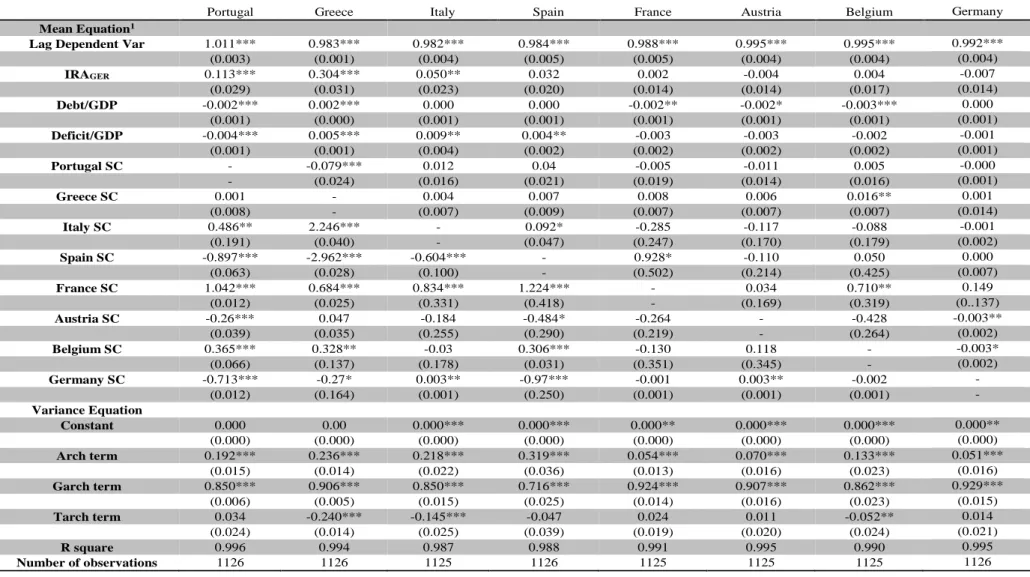
Results
9
Looking at the results it is possible to observe a different impact (of contagion and investors’ risk aversion) on Southern and Central European countries’ yields. The main difference consists in the IRA variable since an increase in investors’ risk aversion has a positive and significant impact on Portugal, Italy and Greece’s yields while in case of the Central European countries’ yields that factor does not play such a vital role and is not even statistically significant. It is also worth noting that country’s specifics, like debt and government deficits, do not exert as crucial influence on yields as contagion and investors’ risk aversion.
The results of the contagion variable indicate that contamination between Southern European banks has, in general, a significantly negative or non-significant impact, except for Italian banks that are the only source of contagion making yields increase. This may suggest that investors looked at Portugal, Greece and Spain as investment substitutes, which means that if the risk of the financial sector in one country increases, investors will look for a substitute investment. This will in turn result in an increase in bonds’ prices of this substitute investment, and consequently decreasing yields.
Contagion from Southern to Central Europe is in general non-significant. Nonetheless in some cases it is significantly positive. This suggests that an increase in the financial sector’s risk in the Southern European countries has a more negative impact on Central European countries’ yields than on the yields of other periphery countries.
The contagion between Central European countries is in general either significantly positive or non-significant, demonstrating that investors perceive those countries as complement investments. The German case is the only one where contagion always decreases yields, proving its “safe-heaven” status.
The main source of yields’ variation, in terms of contagion impact, is the contagion from Central to Southern Europe. If the financial sectors’ risk in Central European countries increases periphery countries’ yields will rise and the majority of the coefficients will be significantly positive.
The results of the study, in particular the results of the contagion variable, contradict some findings in the literature. Arghyrov and Kontonikas (2012) found that contagion in intra periphery countries was the main reason for the divergence between peripheral and core countries in Europe, while Giordano, Pericoli and Tommasino (2013) concluded that contagion was caused by investors starting to pay more attention to specific country’s factors that contributed to the outbreak of the Greek crisis, and so the effects were stronger on periphery countries.
This paper’s results, on the contrary, suggest that the main source of yields divergence is risk aversion and not contagion. However the findings also indicate that even contagion between Central and Southern European countries is stronger than contagion between Southern countries, which is not a source of divergence, as Arghyrov and Kontonikas (2012) and Giordano, Pericoli and Tommasino (2013) claimed. This may be justified with the approach adopted in this paper, which allows us to differentiate between pure contagion and investors’ risk aversion.
What supports the statement that the differences between the results comes from the separation between contagion and risk aversion is also the impact of the IRA variable. It has been demonstrated that the risk aversion has a stronger and more significant impact on Southern European countries than on the Central ones, which is in line with the contagion results presented in other papers. It may indicate that contagion and risk aversion were being confused with one another.
Other reason why the results may differ from the ones of the studies presented above is that in this paper the contagion between banks, and not sovereigns, is being analyzed. Nevertheless, Stânga
10
(2014) establishes the link between sovereign and banking risk, demonstrating that the increase of a bank’s risk or a banking bailout will also contribute to the augmentation of the sovereign’s risk.
Acharya, Drechsler and Schnabl (2013) illustrated as well that banking and sovereign’s risk followed a similar path, which may indicate that the effect of sovereign and banking contagion on sovereign yields may not be that different.
With this in mind, the SC variable may capture a channel of contagion between sovereigns, the financial sector one. The increase of a bank’s risk in country i will contribute to the higher risk of the sovereign in this country. As the sovereign’s risk in country i increases, bank’s risk in country B may increase as well. Bolton and Jeanne (2011) demonstrated that banks, trying to diminish their exposure to an individual country’s sovereign, diversify their portfolios. As a result, if sovereign’s risk in country i increases, the bank in country j is likely to be exposed to it and its risk will rise as well, which consequently affects the sovereign’s risk in country j. It is therefore possible to conclude that the difference between results presented in this study and the ones provided in other studies derives from the differentiation between contagion and investors’ risk aversion, and not the fact that this paper measures banking contagion instead of sovereign contagion.
The advantage of measuring banking and not sovereign contagion is that it may help prevent endogeneity problems (analyzed in section 6).
4. Impact of banking contagion and risk aversion during sovereign bailouts
Gennaioli, Martin and Rossi (2013) studied the impact of sovereign bailouts on domestic banks. They found that government bailouts are costly as they destroy domestic banks’ balance sheets.
The aim of this section is to evaluate if the impact of sovereign bailouts on domestic banks is transmitted to foreign banks and if this transmission mechanism has an impact on foreign government yields. The bailout events to be analyzed are the following: the two Greek bailouts as well as the debt restructure, the Portuguese and the Spanish banks bailouts.
With the methodology used it will be possible to distinguish if it was the risk aversion or the banking contagion that caused the yields divergence between Central and Southern European countries during these events. The results will strengthen even more the conclusions drawn in the previous section as they indicate that this divergence is mainly caused by investors’ risk aversion and not contagion.
There is some literature studying how specific events occurring in one country spread to other countries. Over the years following the establishment of the Euro Area some warnings were issued for some countries that were not respecting the rules of the Maastricht treaty. However, Codogno, Favero and Missale (2003) found that although the Portuguese spreads reacted to a warning issued in 2002, no other country responded to this or other warnings.
Similarly Giordano, Pericoli and Tommasino (2013) studied three political decisions adopted by the EU. The first was the introduction of the European Financial Stability Facility (EFSF). The second was the introduction of the European Stability Mechanism (ESM) and the last one was the decision to provide Greece with a new financial assistance program. They found that while the first decision eased the tensions in Europe the second had the opposite effect, which may have been caused by the Greek and Irish bailout.
11
Cobert (2014) evaluated the impact of sovereign rating downgrades on government debt to find out that the downgrade of the rating of a sovereign contributed to the yields’ increase throughout European countries.
Mink and de Haan (2012) studied the impact of the Greek news on government and bank bonds. They were evaluating the news for twenty days with extreme returns on Greek bonds, to find out that only the Greek bailouts had an impact on sovereign and bank bonds, even on banks that have no exposure to Greece.
Methodology
The methodology used at this stage will be the same as the one applied in the model in section 3 since the objective is still to differentiate between the impact of contagion and investors’ risk aversion, and the problems with the data are still the same. As the aim is to observe the contagion coming from countries where the bailouts took place, the impact on the government bonds of the country where the event occurs will not be evaluated.
To catch the contagion during these events the following two dummy variables will be introduced: one equal to one on the day of the event and the following four week days, and other equal to one on the five week days before the event to control for expectations. These two dummies are then multiplied by the contagion variable of the country where the event takes place to isolate the impact of this variable during this period of time.
The regression will be estimated during a period starting 30 week days before the event and ending 30 week days after, as usually done on the event literature. The regression will take the following form Mean equation 𝑟𝑖𝑡 = 𝛽0+ 𝛽1(𝑟𝑖𝑡−1) + 𝛽2𝑃𝑢𝑏𝑙𝑖𝑐 𝐷𝑒𝑏𝑡 𝐺𝐷𝑃 𝑖𝑡+ 𝛽3 𝐵𝑢𝑑𝑔𝑒𝑡 𝐷𝑒𝑓𝑖𝑐𝑖𝑡 𝐺𝐷𝑃 𝑖𝑡+ 𝛽4(𝐼𝑅𝐴𝐺𝐸𝑅𝑡) + ∑𝑗,𝑘𝛽𝑘𝑆𝐶𝑗𝑡+ 𝛽11(𝑆𝐶ℎ𝑡∗ 𝑏𝑒𝑓𝑜𝑟𝑒 𝑒𝑣𝑒𝑛𝑡ℎ) + 𝛽11(𝑆𝐶ℎ𝑡∗ 𝑒𝑣𝑒𝑛𝑡ℎ) + 𝜀𝑖𝑡 𝑗 ≠ ℎ ≠ 𝑖 (2) Variance Equation 𝑉𝑎𝑟(𝜀𝑖𝑡|Ω𝑖𝑡−1) = 𝜎𝑖𝑡2 = 𝜔 + 𝜃𝜀𝑖𝑡−12 + 𝛾𝜎𝑖𝑡−12 + 𝛼𝜀𝑖𝑡−12 𝐼(𝜀𝑖𝑡−1 < 0)
where h stands for the country where the event takes place, i the country in study and j all the other countries in the sample, and t the period.
The variables of interest will be the IRA and the dummies multiplied by the SC variable of the country where the event takes place. All the other variables are incorporated as control variables.
Results
The results of equation (2) are presented in Table II (annex III). The overall results of the event study support the conclusions of Section 3 that the investors’ risk aversion, and not contagion, is the main source of divergence.
Usually, during these events Southern European countries’ yields rise more than these of the Central European countries. Mink and de Haan (2012) concluded that the Greek bailouts and the Greek news had a stronger impact on Portugal, Spain and Ireland than on the other European countries.
12
Those conclusions are in line with the results for the Greek bailouts and debt restructure presented in this paper which determine that the Greek bailouts and the Greek news exerted much stronger influence on Portugal, Italy and Spain than on Austria, Belgium, France and Germany. The advantage of the methodology used in this paper is that it allows us to understand why these differences arise.
The results indicate that the main differences come about due to a stronger impact of investors’ risk aversion on the periphery countries than on the core countries. Contagion has a similar impact throughout all European countries in sample making yields increase, which is in line with the findings of Mink and Haan (2012) who stated that even banks with no exposure to Greece were affected by the bailouts. In contrast, risk aversion affects almost exclusively Portugal, Spain and Italy. Comparing those results with the impact of risk aversion measured in Section 3, it is possible to conclude that the price of risk demanded by investors has an even stronger impact during these events than during the overall period.
Portuguese and Spanish bailouts illustrate that difference even more explicitly. The results indicate that whereas contagion resulted in the increase of yields in the Central European countries, it made yields decrease in the other Southern European countries. This may show that Central European banks were more exposed to the Portuguese and Spanish situation. However, the impact of risk aversion, which is stronger than the impact of contagion, causes an increase of the Southern European countries’ yields.
The impact of risk aversion on Austria, Belgium and France governments’ yields is even negative in some cases, which demonstrates the fact that investors move from periphery to these countries during these events. The IRA for Germany illustrates this move even more explicitly, and confirms the “safe-haven” status of Germany, as it has always a negative impact on the German yields.
Consequently, the results of the event study allows to see more clearly the difference between contagion and risk aversion and presents even more evidence that investors risk aversion is the main cause of divergence between Southern and Central European countries’ yields.
5. Discussion
The conclusions drawn from the results of the overall period analysis indicate that risk aversion has a stronger impact on yields than both contagion and the country’s specifics included in the regression. The results of the event study strengthen this conclusion and show that during these events investors’ risk aversion influences yields to even a greater degree.
Our methodology also allowed us to differentiate between contagion and investors risk aversion, two variables that are many times confused with one another in the literature. The results indicate that risk aversion was the main cause of divergence between Central and Southern European countries. Banking contagion has a similar impact throughout all European countries, which may indicate that banks in different countries are exposed to foreign countries/banks to the same degree. What would be interesting to understand is why investors’ risk aversion had a much stronger and more significant impact on Southern European country yields. The fact that the country’s specific variables have a diminished impact on yields, according to the results presented in this paper, may ensue from the introduction of investors’ risk aversion. Thus, as specifics were worse in case of the Southern countries, investors’ risk aversion had a greater impact on those countries’ yields.
13
In the literature it is shown that with the formation of monetary union country specifics lost their importance. Pozzi and Wolswijk (2008) studied the period between 1995 and 2006 to find out that with the introduction of the Euro country specific factors such as debt to GDP ratio or deficits, started to lose their significance when evaluating the determinants of sovereign interest rates. In 2006, in the EMU, country specific factors also did not play an important role, a position supported by Bernoth and Erdogan (2010). Nonetheless we could observe that with the outbreak of the financial crisis the country specific factors regained importance, evidence presented by Mody (2009).
The introduction of risk aversion in our specification may have contributed to the smaller impact of specifics on yields. Some of the impact of those variables may be explained by the investors’ behavior. As specifics become negative, less investors want to invest in the country.
Ang and Bekaert (1998) demonstrated that sovereign yields have two different regimes, and that those regimes are associated with GDP growth rates regime. The behavior of yields during the expansion is different from the behavior during the recession.
Those two different regimes may be associated with investors’ risk aversion. In one regime, as macro specific variables of one country present worth results, investors become more risk averse with respect to that country, while in the other regime investors’ do not pay much attention to country specific factors and attach more importance to global factors.
As the literature shows, with the establishment of the European Monetary Union country specifics lost their importance and there were minor spreads differential between European countries. Consequently, during “regular” times, country specific do not play an important role and there wouldn’t be therefore major differences between country spreads caused by investors’ risk aversion. That period of time may represent one regime. With the outbreak of the financial crisis, countries’ specifics regained importance according to some literature. The financial crisis may have represented a change of regime for some countries that presented worse fundamentals.
The second regime is caught in the results of this paper. As only the crisis period is being analyzed, it is possible to observe that the Southern countries are in a different regime, with investors risk aversion being the main driver of sovereign yields in these countries. A change of regimes and the importance that investors attach to the country’s specific variables are the main reasons why investors’ risk aversion has divergent consequences in different countries.
Even though this study helps us understand the differences between contagion and risk aversion, further investigation is needed to better understand the different impact of investors’ risk aversion on different countries’ yields and what triggers the change of investors’ behavior.
6. Robustness test
In order to check the validity of the results two different robustness tests are performed.
Firstly, we noticed a parallel between the majority of the results as the coefficients associated with the lag of the independent variable are close to one, which may indicate the presence of a unit root in this variable.
In order to test if this affects the results a regression, with the lag of the interest rate differentials now as the dependent variable and no lag of the dependent variable incorporated as an explanatory variable, will be estimated. This robustness test is computed for both the entire period and event specifications.
14
The results of this new regression indicate that the majority of the conclusions are not affected by the presence of a unit root on the lag of the dependent variable. However there is one country where almost all results change sign and significance, which is Austria. This may indicate that the presence of a unit root on the lag of the dependent variable affects the results for this country.
For the events specifications the changes in results are even more subtle. The majority of the signs of interest do not change, the impact of the relevant variables stay similar and with the same statistical significance. As a result, the conclusions for the events specifications are not affected as well.
Secondly, it was noticed that there was the possibility of existence of endogeneity in the results. As SC variables are extracted from the banks’ CDS spreads, these spreads may be correlated to sovereign yields, which may cause endogeneity between the SC variable and the yields.
The difficulty in testing endogeneity consists in the instrument choice as there is a need to guarantee that the instrumental variable is connected with the SC variables but that is not affected by sovereign yields. We find the best instrument is European Central Bank reference interest rates as they are not affected by sovereign yields but may affect the CDS spreads and consequently the SC variables.
To test endogeneity regressions (1) and (2) were estimated with some modifications. First the SC variable was used as the dependent variable and the instrument as an independent variable. Then the residuals of this new regression were added in regressions (1) and (2), and if the impact of the residuals was significantly different from zero we could speak about endogeneity.
The broad majority of the results indicates that no endogeneity is present. Nevertheless in case of Greece, there is endogeneity in the banking contagion coming from Portugal, Austria, Belgium, Germany and France. This may indicate that Greek government was more exposed to banking risk and that banks had also a high exposure to the Greek situation.
In case of the Belgian and Italian situation we could also observe some endogeneity, but a week one (only considering an interval of confidence of 10%). For Belgium coming from Portugal, Spain and Italy and for Italy coming from Austria and Spain. However it is possible to state that the endogeneity does not affect the regressions’ results for these two countries.
As a consequence, we can conclude that only in the Austrian and Greek cases results may not be valid but that the overall conclusions of the paper are not affected by unit roots or endogeneity.
7. Conclusions
The aim of this paper was to distinguish between the impact of contagion through financial sector channels and investors’ risk aversion, both during the entire period of crisis and during sovereign bailouts. Results indicate that investors’ risk aversion was the main driver of the differences between Central and Southern European countries’ yields, with contagion affecting in a similar way all countries in the sample.
It was possible to conclude as well that the difference in the impact of investors’ risk aversion may come about due to the different regimes where some countries find themselves. These different regimes may be triggered by a worsening of country’s specifics, which have a small impact on yields.
15
Those conclusions have some policy implications. The Southern Europe countries considered in the analysis should focus on achieving long-term financial stability. As investors, started paying more attention to the countries’ specifics after the crisis broke out, Greece, Portugal, Spain and Italy were the ones more affected by the change in investors’ behavior. That may have led to a change of regime. Moreover, as the paper’s results show, risk premiums is the main driver of sovereign interest rates in those countries. So, in order to restore trust of the investors and bring the “regular” regime back the periphery countries should therefore focus on financial stability.
Equally the European Union should react more strongly to financial instability or default of a country in order to prevent spreading these phenomena to other countries as the bailouts did. If the bailouts contagion to the other Southern Europe countries had not been so strong, those countries would have probably been in a better situation during the period studied in this paper. As we have seen contagion affects all the European countries in the sample. This is not a desirable situation. Accordingly, EU should take measures to prevent contagion. In order to reach this goal, EU should control the financial sector transmission channels, probably by increasing the integration of the financial sector in Europe, which at the same time guarantees more effective regulations and a more tightened supervision of financial institutions. Countries should also look for new financing ways in order to guarantee that neither sovereigns nor the economy are dependent on the financial sector to such a degree, which would probably decrease the financial sector contagion and its impact.
16 References
Acharya, V.; Drechsler, I. and Schnabl, P. (2014). “A Pyrrhic Victory Bank Bailouts and Sovereign Credit Risk”, The Journal of Finance;
Afonso, A.; Arghyrou, M. and Kontonikas, A. (2012). “The determinants of sovereing bond yield spreads in the EMU”, School of Economics and Management, Technical University of Lisbon WP 36/2012/DE/UECE;
Alper, C.; Forni, L. and Gerard, M. (2012). “Pricing of Sovereign Credit Risk: Evidence from Advanced Economies during the Financial Crisis”, IMF Working Paper WP/12/24;
Ang, A. and Bekaert, G. (2002). “Regime Switches in interest rates”, Journal of Business & Economic Statistics;
Arghyrou, M. and Kontonikas, A. (2011). “The EMU sovereign-debt crisis: Fundamentals, expectations and contagion”, European Commission Economic Papers 436;
Audrino, F.; De Georgio, E. and Filipova, K. (2014). “Monetary policy regimes Implications for the yield curve and bond pricing”, Journal of Financial Economics;
Baek, I.; Bandopadhyaya, A. and Du, C. (2005). “Determinants of market-assessed sovereign risk: Economic fundamentals or market risk appetite?”, Journal of International Money and Finance 24 (2005) 533-548;
Beirne, J. and Fratzscher, M. (2013). “The pricing of sovereign risk and contagion during the European sovereign debt crisis”, Journal of International Money and Finance;
Bernoth, K. and Erdogan, B. (2010). “Sovereign bond yield spreads: A time-varying coefficient approach”, European University Viadrina Frankfurt, Deparment of Business Administration and Economics Discussion Paper No. 289;
Bernoth, K.; von Hagen, J. and Schuknecht, L. (2004). “Sovereign Risk Premia in the European Government Bond Market”, European Central Bank, Working Paper Series No. 369;
Bernoth, K.; von Hagen, J. and Schuknecht, L. (2006). “Sovereign Risk Premiums in the European Government Bond Market”, Governance and the Efficiency of Economic Systems, Discussion Paper No. 151;
Bernoth, K and Wolff, G. (2006). “Fool the markets? Creative accounting, fiscal transparency and sovereign risk premia”, Deutsche Bundesbank, Discussion Paper Series 1: Economic Studies No 19/2006;
Bolton, P and Jeanne, O. (2011). “Sovereign Default Risk and Bank Fragility in Financially Integrated Economies”, IMF Economic Review;
Brutti, F. and Sauré, P. (2011). “Transmission of Sovereign Risk in the Euro Crisis”, University of Zurich Working Paper No. 108;
Buiter, W and Grafe, C. (2003). “EMU or Ostrich?”;
Caceres, C.; Guzzo, V. and Segoviano, M. (2010). “Sovereign Spreads: Global Risk Aversion, Contagion or Fundamentals?”, IMF Working Paper WP/10/120;
Codogno, L; Favero, C. and Missale, A. (2003). “Yield spreads on EMU government bonds”, Economic Policy, Volume: 37 pp.503-531;
17
Corbet, S. (2014). “The Contagion Effects of Sovereign Downgrades”, International Journal of Economics and Financial Issues;
Di Cesare, A.; Grande, G.; Manna, M. And Taboga, M. (2012). “Recent estimates of sovereign risk premia for euro-area countries”, Banca d’Italia Working Paper Number 128;
Dotz, N and Fischer, C. (2010). “What can EMU countries’ sovereign bond spreads tell us about market perceptions of default probabilities during the recent financial crisis?”, Deutsche Bundesbank, Discussion Paper Series 1: Economic Studies No 11/2010;
Eichler, S. and Maltritz, D (2012). “The term structure of sovereign default risk in the EMU member countries and its determinants”, Journal of Banking & Finance;
Ejsing, J. and Lemke, W. (2011), “The Janus-Headed Salvation: Sovereign and Bank Credit Risk Premia during 2008-2009”, Economics Letters, 110(1), 28-31.
Espinoza, R. and Segoviano, M. (2011). “Probabilities of Default and the Market Price of Risk in a Distressed Economy”, IMF Working Paper WP/11/75;
Featherstone, K. (2011). “The Greek Sovereign Debt Crisis and EMU: A Failing State in a Skewed Regime”, JCMS 2011 Volume 49. Number 2. Pp. 193-217;
Fontana, A and Scheicher, M (2010). “An Analysis of Euro Area Sovereign CDS and their Relation with Government Bonds”, European Central Bank, Working Paper Series No 1271;
Gabrisch, H. and Orlowski, L. (2009). “Interest Rate Convergence in the Euro-Candidate Countries: Volatility Dynamics of Sovereign Bond Yields”, WCOB Working Papers Paper 2;
Gennaioli, N.; Martin, A. and Rossi, S. (2014). “Sovereign Default, Domestic Banks, and Financial Institutions”, The Journal of Finance;
Giordano, R.; Pericoli, M and Tommasino, P. (2013). “Pure or wake-up-call contagion? Another look at the EMU sovereign debt crisis”, Banca d’Italia Working Paper Number 904;
Guerreiro, D. and Mignon, V. (2011). “On price convergence in Eurozone”, Economix Working Paper 2011-34;
Haan, J. de and Mink, M. (2013). “Contagion during the Greek Sovereign Debt Crisis”, Journal of International Money and Finance;
Hein, E. and Truger, A. (2003). “European Monetary Union: nominal convergence, real divergence and slow growth?”, Structural Change and Economic Dynamics 16 (2005) 7-33;
Honohan, P. and Lane, P. (2003). “Divergent Inflation Rates in EMU”, Trinity Economics Papers No. 20034;
Lane, P. (2006). “The Real Effects of EMU”, IIIS Discussion Paper No. 115;
Longstaff, F; Pan, J.; Pedersen, L and Singleton, K. (2011). “How Sovereign is Sovereign Credit Risk?”, American Economic Journal: Macroeconomics 3: 75-103;
Martinez, L.; Terceño, A. and Teruel, M. (2012). “A Sovereign Bond Spreads Analysis in the European Union and European Monetary Union: a Panel Data Framework”, Universitat Rovira I Virgili;
Pagano, M. (2004). “The European Bond Markets under EMU”, Oxford Review of Economic Policy, Vol. 20, No.4;
18
Pan, J. and Singleton, K. (2008). “Default and Recovery Implicit in the Term Structure of Sovereign CDS Spreads”, The Journal of Finance;
Pozzi, L. and Sadaba, B. (2012). “Did the financial crisis cause a regime shift in euro area government bond risk pricing?”;
Sbracia, M. (2003). “A Primer on Financial Contagion”, Journal of Economic Surveys Vol.17 No. 4;
Segoviano, M. (2006). “Consistent Information Multivariate Density Optimizing Methodology”, Financial Markets Group;
Stânga, I. M. (2014). “Bank bailouts and bank-sovereign risk contagion channels”, Journal of International Money and Finance;
Suh, S. (2013). “Measuring Sovereign Risk Contagion in the Eurozone”, Chung-Ang University;
19
Annex I – Spillover Coefficient
To illustrate the CIMDO method we will focus on an example of a portfolio of loans granted to two different investors, each one with logarithmic returns given by x and y. The objective function is defined as
𝐶[𝑝, 𝑞] = ∫ ∫ 𝑝(𝑥, 𝑦)𝑙𝑛 [𝑝(𝑥, 𝑦)
𝑞(𝑥, 𝑦)] 𝑑𝑥 𝑑𝑦
where q(x,y) stands for the prior distribution and p(x,y) the posterior distribution.
As the CIMDO method assumes that default occurs when the asset value of a firm drops below a certain threshold, we may assume that the portfolio follows a multivariate distribution q(x,y)∈ 𝑅2 that is normal N(0,I), where I is the identity matrix, which is consistent with the economic intuition behind the CIMDO method.
To find the thresholds we will compute an average of the default threshold through time, which will be given by
𝑋𝑑𝑥 = Φ−1(1 − 𝑃𝑜𝐷̅̅̅̅̅̅𝑥) and 𝑋 𝑑
𝑦
= Φ−1(1 − 𝑃𝑜𝐷̅̅̅̅̅̅𝑦)
where Φ is the inverse of a standard normal cumulative distribution function.
Having the thresholds we can now estimate the moment-consistency constraints ∫ 𝑝(𝑥)𝕀[𝑋 𝑑𝑥,∞)𝑑𝑥 = 𝑃𝑜𝐷𝑡 𝑥 ∫ 𝑝(𝑦)𝕀[𝑋 𝑑 𝑦 ,∞)𝑑𝑦 = 𝑃𝑜𝐷𝑡 𝑦
with 𝑝(𝑥) 𝑎𝑛𝑑 𝑝(𝑦) being the posterior probability density functions and 𝕀[𝑋 𝑑 𝑦
,∞) and 𝕀[𝑋𝑑𝑥,∞) being the indicator functions defined by
𝕀[𝑋
𝑑𝑖,∞) = {
1 𝑖𝑓 𝑖 ≥ 𝑋𝑑𝑖
0 𝑖𝑓 𝑖 < 𝑋𝑑𝑖 , 𝑖 = 𝑥, 𝑦
However as the objective is to obtain the joint posterior distribution we will calculate ∫ ∫ 𝑝(𝑥, 𝑦)𝕀[𝑋 𝑑𝑥,∞)𝑑𝑥 𝑑𝑦 = 𝑃𝑜𝐷𝑡 𝑥 ∫ ∫ 𝑝(𝑥, 𝑦)𝕀[𝑋 𝑑 𝑦 ,∞)𝑑𝑦 𝑑𝑥 = 𝑃𝑜𝐷𝑡 𝑦
The last constraints that will need to be satisfied are the probability additivity constraints 𝑝(𝑥, 𝑦) ≥ 0
∫ ∫ 𝑝(𝑥, 𝑦)𝑑𝑥 𝑑𝑦 = 1 to ensure that p(x,y) is a valid density.
20 min 𝑝(𝑥,𝑦)∫ ∫ 𝑝(𝑥, 𝑦)𝑙𝑛 [ 𝑝(𝑥,𝑦) 𝑞(𝑥,𝑦)] 𝑑𝑥 𝑑𝑦 𝑠. 𝑡 ∫ ∫ 𝑝(𝑥, 𝑦)𝕀[𝑋 𝑑𝑥,∞)𝑑𝑥 𝑑𝑦 = 𝑃𝑜𝐷𝑡 𝑥 ∫ ∫ 𝑝(𝑥, 𝑦)𝕀[𝑋 𝑑 𝑦 ,∞)𝑑𝑦 𝑑𝑥 = 𝑃𝑜𝐷𝑡 𝑦 𝑝(𝑥, 𝑦) ≥ 0 ∫ ∫ 𝑝(𝑥, 𝑦)𝑑𝑥 𝑑𝑦 = 1 Setting up the Lagrangian equation
𝐿(𝑝, 𝑞) = ∫ ∫ 𝑝(𝑥, 𝑦)𝑙𝑛 [𝑝(𝑥, 𝑦) 𝑞(𝑥, 𝑦)] 𝑑𝑥 𝑑𝑦 + 𝜆1[∫ ∫ 𝑝(𝑥, 𝑦)𝕀[𝑋𝑑𝑥,∞)𝑑𝑥 𝑑𝑦 − 𝑃𝑜𝐷𝑡 𝑥] + 𝜆2[∫ ∫ 𝑝(𝑥, 𝑦)𝕀[𝑋𝑑𝑦,∞)𝑑𝑦 𝑑𝑥 − 𝑃𝑜𝐷𝑡 𝑦 ] + 𝜇 [∫ ∫ 𝑝(𝑥, 𝑦)𝑑𝑥 𝑑𝑦 − 1] which can be simplified to
𝐿(𝑝, 𝑞) = ∫ ∫ 𝑝(𝑥, 𝑦)[ln 𝑝(𝑥, 𝑦) − ln 𝑞(𝑥, 𝑦)]𝑑𝑥 𝑑𝑦 + ∫ ∫ 𝑝(𝑥, 𝑦) [𝜆1𝕀[𝑋𝑑𝑥,∞)+ 𝜆2𝕀[𝑋 𝑑 𝑦 ,∞)+ 𝜇] 𝑑𝑦 𝑑𝑥 − 𝜆1𝑃𝑜𝐷𝑡𝑥− 𝜆2𝑃𝑜𝐷𝑡 𝑦 − 𝜇 we can reach the optimum by performing the following variation
𝛿𝐿 =𝑑𝐿[𝑝(𝑥, 𝑦) + 𝜀𝛾(𝑥, 𝑦), 𝑞(𝑥, 𝑦)]
𝑑𝜀 |
𝜀=0 = 0
with 𝜀 being very small and 𝛾(𝑥, 𝑦) a continuous function equal to zero at the boundary of integration and finite variance.
The optimal solution will be then given by
𝑝(𝑥, 𝑦)̂ = 𝑞(𝑥, 𝑦)𝑒𝑥𝑝 {− [1 + 𝜇̂ + 𝜆̂𝕀1 [𝑋
𝑑𝑥,∞)+ 𝜆̂𝕀2 [𝑋𝑑𝑦,∞)]}
With the results of 𝑝(𝑥, 𝑦)̂ and q(x,y) we can now replace them on the objective function and achieve the joint probability of default.
21 Annex II – Index of Global Risk Aversion
Estimating IGRA: 𝐼𝐺𝑅𝐴 = −(1 − 𝑃𝑜𝑅𝑡) = − (1 −𝑉𝑜𝑙𝑎𝑡𝑖𝑙𝑖𝑡𝑦 𝑜𝑓 𝑚𝑡 𝜋𝑡 ) = − (1 − 𝑉𝑎𝑟(𝑚𝑡+1) 𝐸[𝑚𝑡+1] 𝜋𝑡 )
Accordingly, we need 𝜋𝑡, 𝑉𝑎𝑟(𝑚𝑡+1) and 𝐸[𝑚𝑡+1]. First: Estimate the mean of mt+1 using
𝑅𝑡+1𝑓 = 1 𝐸[𝑚𝑡+1]
𝑅𝑡+1𝑓 − 𝑃𝑟𝑜𝑥𝑖𝑒𝑑 𝑓𝑟𝑜𝑚 𝑂𝐼𝑆 (𝑜𝑣𝑒𝑟𝑛𝑖𝑔ℎ𝑡 𝑖𝑛𝑑𝑒𝑥 𝑠𝑤𝑎𝑝) 𝑟𝑎𝑡𝑒 Second: Estimate 𝑉𝑎𝑟(𝑚𝑡+1) using the formula
𝜆𝑚 =𝑉𝑎𝑟(𝑚𝑡+1) 𝐸[𝑚𝑡+1]
where 𝜆𝑚 is the price of risk estimated by CAPM excess returns equation 𝐸𝑡[𝑟𝑡+1𝑖 ] − 𝑟𝑡𝑓= 𝛽𝑖,𝑚𝜆𝑚
which can be estimated using Fama-MacBeth regressions.
Another way to estimate the price of risk is by means of the VIX index (Espinoza and Segoviano, 2010). The price of risk can be inferred from the maximum sharp ratio of an efficient portfolio. To prove this we use the pricing equation
𝐸(𝑅𝑖) − 𝑅𝑓 = −𝜌𝑚,𝑅𝑖
𝑉𝑎𝑟(𝑚)
𝐸(𝑚) 𝑉𝑎𝑟(𝑅
𝑖)
As 𝜌𝑚,𝑅𝑖 cannot be higher than 1 |𝐸(𝑅
𝑖) − 𝑅𝑓 𝑉𝑎𝑟(𝑅𝑖) | ≤
𝑉𝑎𝑟(𝑚) 𝐸(𝑚)
The maximum sharp ratio will therefore be equal to the price of risk given by 𝑉𝑎𝑟(𝑚)
𝐸(𝑚)
Historically a Sharpe ratio of 3 or higher would be considered very high, so we normalize the VIX index by 4 to scale it down to consistent levels with price of risk properties.
Third: Estimate 𝜋𝑡 (actual probability of default) using the risk neutral probability of default (𝜋̂) 𝑡 according to the following equation
𝜋𝑡 = 𝜋̂𝑡
(1 + 𝑟𝑡𝑓)𝐸𝑡(𝑚𝑡+1|𝑑𝑖𝑠𝑡𝑟𝑒𝑠𝑠) Where the risk neutral probability can be calculated as
22 𝜋𝑡 ̂ = 𝑆𝑁 (1 − 𝐾) 𝑆𝑁− 𝐶𝐷𝑆 𝑜𝑓 𝑐𝑜𝑢𝑛𝑡𝑟𝑦 𝑁 𝐾 − 𝑟𝑒𝑐𝑜𝑣𝑒𝑟𝑦 𝑟𝑎𝑡𝑒 (𝑎𝑠𝑠𝑢𝑚𝑒𝑑 𝑒𝑞𝑢𝑎𝑙 𝑡𝑜 60%)
As the market price of risk in a stress situation is not observable, by defining stress as the market price of risk above a certain threshold value, and by assuming 𝑚𝑡+1is normally distributed, we can infer from the truncated normal distribution formula that
𝐸𝑡(𝑚𝑡+1|𝑑𝑖𝑠𝑡𝑟𝑒𝑠𝑠) = 𝐸𝑡(𝑚𝑡+1|𝑚𝑡+1> 𝑇) = 𝜇𝑡+ 𝜎𝑡𝜆(α𝑡) where 𝜇𝑡= 𝐸[𝑚𝑡+1] 𝜎𝑡 = 𝑉𝑎𝑟(𝑚𝑡+1) 𝜆 = 𝜑(𝛼) [1 − Φ(α)]
Φ − normal comulative distribution function 𝜑 − normal distribution density function
α𝑡= 𝑡ℎ𝑟𝑒𝑠ℎ𝑜𝑙𝑑 − 𝜇𝑡 𝜎𝑡 with the threshold being given by
𝑇 = 𝐸[𝑚] + Φ−1[1 − 𝜋 𝑡]√𝑣𝑎𝑟(𝑚) = 1 1 + 𝑟̅+ Φ −1[1 − 𝜋 𝑡]𝜎̅
respectively, the actual probability of default will be given by estimating the non-linear equation 𝜋𝑡 = 𝜋𝑡 ̂ 1 + (1 + 𝑟𝑡𝑓)𝜎𝑡∗ 𝜆 ( 1 1 + 𝑟̅ − 1 1 + 𝑟𝑡𝑓+ Φ −1[1 − 𝜋 𝑡]𝜎̅ 𝜎𝑡 )
23 Annex III – Results
Table 1 – Risk aversion vs banking contagion4
4 *** - Statistically significant at 1%; ** - Statistically significant at 5%; * - Statistically significant at 10%
1 *** - Statistically significant at 1%; ** - Statistically significant at 5%; * - Statistically significant at 10%
Portugal Greece Italy Spain France Austria Belgium Germany
Mean Equation1
Lag Dependent Var 1.011*** 0.983*** 0.982*** 0.984*** 0.988*** 0.995*** 0.995*** 0.992***
(0.003) (0.001) (0.004) (0.005) (0.005) (0.004) (0.004) (0.004) IRAGER 0.113*** 0.304*** 0.050** 0.032 0.002 -0.004 0.004 -0.007 (0.029) (0.031) (0.023) (0.020) (0.014) (0.014) (0.017) (0.014) Debt/GDP -0.002*** 0.002*** 0.000 0.000 -0.002** -0.002* -0.003*** 0.000 (0.001) (0.000) (0.001) (0.001) (0.001) (0.001) (0.001) (0.001) Deficit/GDP -0.004*** 0.005*** 0.009** 0.004** -0.003 -0.003 -0.002 -0.001 (0.001) (0.001) (0.004) (0.002) (0.002) (0.002) (0.002) (0.001) Portugal SC - -0.079*** 0.012 0.04 -0.005 -0.011 0.005 -0.000 - (0.024) (0.016) (0.021) (0.019) (0.014) (0.016) (0.001) Greece SC 0.001 - 0.004 0.007 0.008 0.006 0.016** 0.001 (0.008) - (0.007) (0.009) (0.007) (0.007) (0.007) (0.014) Italy SC 0.486** 2.246*** - 0.092* -0.285 -0.117 -0.088 -0.001 (0.191) (0.040) - (0.047) (0.247) (0.170) (0.179) (0.002) Spain SC -0.897*** -2.962*** -0.604*** - 0.928* -0.110 0.050 0.000 (0.063) (0.028) (0.100) - (0.502) (0.214) (0.425) (0.007) France SC 1.042*** 0.684*** 0.834*** 1.224*** - 0.034 0.710** 0.149 (0.012) (0.025) (0.331) (0.418) - (0.169) (0.319) (0..137) Austria SC -0.26*** 0.047 -0.184 -0.484* -0.264 - -0.428 -0.003** (0.039) (0.035) (0.255) (0.290) (0.219) - (0.264) (0.002) Belgium SC 0.365*** 0.328** -0.03 0.306*** -0.130 0.118 - -0.003* (0.066) (0.137) (0.178) (0.031) (0.351) (0.345) - (0.002) Germany SC -0.713*** -0.27* 0.003** -0.97*** -0.001 0.003** -0.002 - (0.012) (0.164) (0.001) (0.250) (0.001) (0.001) (0.001) - Variance Equation Constant 0.000 0.00 0.000*** 0.000*** 0.000** 0.000*** 0.000*** 0.000** (0.000) (0.000) (0.000) (0.000) (0.000) (0.000) (0.000) (0.000) Arch term 0.192*** 0.236*** 0.218*** 0.319*** 0.054*** 0.070*** 0.133*** 0.051*** (0.015) (0.014) (0.022) (0.036) (0.013) (0.016) (0.023) (0.016) Garch term 0.850*** 0.906*** 0.850*** 0.716*** 0.924*** 0.907*** 0.862*** 0.929*** (0.006) (0.005) (0.015) (0.025) (0.014) (0.016) (0.023) (0.015) Tarch term 0.034 -0.240*** -0.145*** -0.047 0.024 0.011 -0.052** 0.014 (0.024) (0.014) (0.025) (0.039) (0.019) (0.020) (0.024) (0.021) R square 0.996 0.994 0.987 0.988 0.991 0.995 0.990 0.995 Number of observations 1126 1126 1125 1126 1125 1125 1125 1126
24 Table 2 – Events results5
5 *** - Statistically significant at 1%; ** - Statistically significant at 5%; * - Statistically significant at 10%
Greece Bailout Second Greece Bailout Greece Debt Restructure Portugal Bailout Spain Bailout Austria SC*Before 0.02** -0.003 0.03*** -0.004 0.02 SC*Event 0.02 -0.01 0.02* 0.02 -0.01 IRA 0.32*** -0.27 -0.60*** -1.58*** 0.36 Belgium SC*Before 0.02* 0.01 -0.001 -0.004 0.01 SC*Event 0.02 -0.01 0.02* -0.002 0.03 IRA 0.22 1.28 0.99*** -0.65 0.67** France SC*Before 0.01 0.01 0.03*** 0.01 0.02 SC*Event 0.01 0.002 0.03* 0.01* 0.01 IRA -0.32 -0.06 0.11 -1.83*** 0.65*** Germany SC*Before 0.002 0.02** 0.02 0.001 0.01 SC*Event 0.02 0.01 0.01 0.02 0.04** IRA -1.09*** -0.72** -0.95*** -1.60*** -0.49* Greece SC*Before - - - -0.10 -0.04 SC*Event - - - -0.19*** -0.35 IRA - - - 1.17 9.68*** Italy SC*Before 0.02 0.04** 0.01 0.01 -0.05 SC*Event 0.02*** 0.03* 0.003 -0.01 0.09** IRA 0.59*** 3.57*** 2.12*** -0.56 0.76 Portugal SC*Before 0.12*** 0.03 0.23* - 0.06 SC*Event 0.12*** 0.03 0.07 - 0.11 IRA 3.32*** 0.86 3.46*** - 1.13 Spain SC*Before 0.03*** 0.05*** 0.01 0.02 - SC*Event 0.03*** 0.05*** -0.01 -0.03* - IRA 1.08*** 4.65*** 0.17 1.25* -
Nova School of Business and Economics
Faculdade de Economia Universidade Nova de Lisboa Campus de Campolide 1099-032 Lisboa PORTUGAL Tel.: +351 213 801 600