Vehicle routing and tour planning problem: a cement industry case study

(1)

Universidade do Minho

Escola de Engenharia

Ricardo David Pereira Alves

Vehicle Routing and Tour Planning

(2)

Universidade do Minho

Dissertação de Mestrado

Escola de Engenharia

Ricardo David Pereira Alves

Vehicle Routing and Tour Planning

Problem: A Cement Industry Case Study

Mestrado em Engenharia de Sistemas

Trabalho realizado sob orientação do

Professor Doutor José António Vasconcelos Oliveira

Professor Doutor Luís Miguel da Silva Dias

(3)

DECLARAÇÃO

Nome: Ricardo David Pereira Alves

Endereço eletrónico: ralves_12_@hotmail.com

Título da dissertação: Vehicle Routing and Tour Planning Problem: A Cement Industry Case Study

Orientadores: Professor Doutor José António Vasconcelos Oliveira e Professor Doutor Luís Miguel Silva Dias

Ano de conclusão: 2018

Mestrado em Engenharia de Sistemas

É

AUTORIZADA

A

REPRODUÇÃO

INTEGRAL

DESTA

DISSERTAÇÃO APENAS PARA EFEITOS DE INVESTIGAÇÃO,

MEDIANTE DECLARAÇÃO ESCRITA DO INTERESSADO, QUE A TAL

SE COMPROMETE.

Universidade do Minho, ___/___/______ Assinatura:

(4)

(5)

(6)

(7)

A

CKNOWLEDGMENTS

Life is like driving a car. This document represents one more road traversed by me. It is therefore necessary to thank all those who helped me in this stage.

First, I want to offer my gratitude to my advisors, J. António Oliveira, Ph.D. and to Luís Dias, Ph.D. for allowing me to grow both academically and personally.

To the University of Minho, for giving me 5 years of great learning.

To my parents, for my education, for the constant support, for teaching me the most important things in the world, and for being an Example to follow everyday.

To Ângela Coutinho, for all the support, patience, friendship, and for encouraging me to be a better person everyday.

To João Fonseca and Ana Regina, for the constant support and for traversing this road together, with me, as colleagues, but, above all, as friends.

Not in order of priority, to my friends José Luís Silva, Afonso Rodrigues, Rui Costa, Miguel Nogueira, Miguel Sanches, Joaquim Santos, José Bruno, Luís Miguel Costa, Ricardo Dias, and João Pedro for the fun moments, and for the learning I had with each one of them.

Finally, I want to show my gratitude to every person who directly, or indirectly, has contributed for the accomplishment of this document.

(8)

(9)

A

BSTRACT

The transportation, being part of the logistics field, plays a crucial role in the business world. Its impact in the costs and service quality is an increasingly imperative topic. In industry, transportation systems are equally important and can represent a large improvement in the management of the plants and in the service quality of the products, thus bringing advantages for the companies and for the clients.

The cement industry is not an exception. Cement is the second most consumed substance in the world and with the great number of trucks arriving at cement facilities, every day, the supply chain management of this industry must encompass this management as well. With the lack of assistance and guidance clients have inside the cement facilities, both companies incur in additional costs and clients experience reduced levels of service quality. To overcome these issues, three algorithms were developed and implemented. Each algorithm has different specifications and different goals. However, all the developed algorithms improve the service quality, guiding the truck drivers – the clients – inside the plants and giving the routes in shorter periods of time. One algorithm guides the trucks through the minimum distance route and will serve as a comparison term for the other two. The other two algorithms, named equilibrium approaches, are the main contribution of this dissertation. These dynamic algorithms consider not only the traveled distance, but also the workload both in the servers and in the roads. The entrance management in the facilities is also a crucial aspect cement companies must be aware of. Several thought policies are presented and an algorithm for the entrance management is developed and implemented. With a simulation software, the developed algorithms were tested and simulated. The simulation results are reported and discussed.

Keywords: Industry 4.0; Supply Chain Management; Vehicle Routing; Tour

(10)

(11)

R

ESUMO

A indústria do transporte desempenha um papel crucial no mundo empresarial. O seu impacto nos custos e na qualidade de serviço são um tópico cada vez mais importante. Na indústria, os sistemas de transporte são igualmente importantes e podem representar uma grande melhoria na gestão das fábricas e na qualidade do serviço dos produtos, trazendo vantagens tanto para as empresas como para os clientes.

A indústria cimenteira não é uma exceção. O cimento é a segunda comodidade mais consumida em todo o mundo, e com o grande número de camiões que chegam às fábricas de cimento todos os dias, a gestão da cadeia de abastecimento desta indústria deve, também, incorporar esta gestão. Com a falta de assistência na orientação que os clientes têm dentro das fábricas, tanto as fábricas incorrem em custos acrescidos como os clientes experienciam uma qualidade de serviço reduzida. Para abordar este problema, três algoritmos foram desenvolvidos e implementados. Cada algoritmo tem objetivos e especificações diferentes. No entanto, todos os algoritmos implementados melhoram a qualidade de serviço guiando os camiões dos clientes dentro das plantas, e calculando as rotas em curtos períodos de tempo. Um dos algoritmos guia os camiões pela rota que permite a menor distância percorrida, e servirá como termo de comparação para os outros dois. Os outros dois algoritmos, chamados abordagens de equilíbrio, são a grande contribuição desta dissertação. Estes algoritmos dinâmicos consideram a ocupação dos servidores e das estradas, além da distância percorrida. A gestão de entrada nas fábricas é também um aspeto importante que as fábricas de cimento devem ter atenção. Diversas políticas de entrada são apresentadas e um algoritmo para a gestão de entrada na fábrica é também desenvolvido e implementado. Com um software de simulação, os algoritmos desenvolvidos foram testados e simulados. Os resultados das simulações são apresentados e discutidos.

Palavras-Chave: Indústria 4.0; Gestão da cadeia de abastecimento; Roteamento

(12)

(13)

C

ONTENTS

ACKNOWLEDGMENTS ... v

ABSTRACT ... vii

RESUMO ... ix

CONTENTS ... xi

LIST OF FIGURES ... xiii

LIST OF TABLES ... xv

LIST OF ACRONYMS ... xvii

1. INTRODUCTION ... 1

2. ROUTING PROBLEMS ... 5

2.1. Introduction ... 5

2.2. Tour Planning ... 6

2.3. Shortest Path Problem ... 7

2.3.1.Dijkstra’s Algorithm ... 9

2.3.2.Floyd-Warshall Algorithm ... 11

2.4. Travelling Salesman Problem ... 13

2.4.1.Outline of the Traveling Salesman Problem ... 13

2.4.2.Travelling Salesman Problem Variations ... 16

3. DYNAMIC VEHICLE ROUTING ... 21

3.1. Outline of the Dynamic Routing Problems ... 21

3.2. Dynamic Shortest Path Problem ... 23

3.3. Traffic Assignment ... 26

3.3.1.Overview ... 26

(14)

3.3.3.Link Cost Functions ... 28

3.3.4.Capacity-Restraint Heuristic ... 30

3.3.5.Incremental Assignment ... 30

4. CEMENT INDUSTRY CASE STUDY ... 33

4.1. List of Publications ... 33

4.2. Cement Industry Overview ... 34

4.3. Industry 4.0 and Cement Industry Supply Chain Management ... 38

4.4. Problem Description ... 40

4.5. Problem Assumptions ... 41

5. APPROACH TO THE PROBLEM & APPLICATIONS ... 43

5.1. Algorithm No.1 – The Distance Approach ... 45

5.2. Algorithm No. 2 – The Equilibrium Approach (without updates) ... 50

5.3. Algorithm No.3 – The Equilibrium Approach (with updates) ... 63

6. IMPLEMENTATION: TESTS AND RESULTS ... 69

6.1. Algorithm No. 1 ... 69

6.2. Algorithm No. 2 ... 70

6.3. Simulation: Algorithms Comparison ... 76

6.4. Discussion ... 80

7. PARKING MANAGEMENT ... 83

8. CONCLUSION AND FUTURE RESEARCH ... 89

BIBLIOGRAPHY ... 93

(15)

L

IST

O

F

IGURES

FIGURE 1 - GENERIC EXAMPLE OF A TOUR PLANNING. ... 7

FIGURE 2 - EXAMPLES OF THE SOP (RIGHT) AND THE TSPPC (LEFT). ... 20

FIGURE 3 - BEST ROUTE AT TIME T1. ... 21

FIGURE 4 - BEST ROUTE AT TIME T0. ... 21

FIGURE 5 - EXAMPLE OF A TIME DEPENDENT SHORTEST PATH. ... 25

FIGURE 6 - TWO ROUTES EXAMPLE FOR THE ALL OR NOTHING ASSIGNMENT. ... 28

FIGURE 7 - INFLUENCE OF TRAFFIC FLOW IN THE TRAVEL TIME OF A ROAD. ... 29

FIGURE 8 - CEMENT INDUSTRY SUPPLY CHAIN. ... 35

FIGURE 9 - CEMENT STORAGE SILO. ... 36

FIGURE 10 - EXAMPLE OF A CISTERN OR TANK TRUCK. ... 37

FIGURE 11 - LOADING TRUCK FOR BAGGED CEMENT. ... 37

FIGURE 12 - INDUSTRY 4.0 IN CEMENT INDUSTRY SUPPLY CHAIN. ... 39

FIGURE 13 - GRAPH EXAMPLE OF A CEMENT FACILITY. ... 43

FIGURE 14 – FLOWCHART OF THE ALGORITHM NO.1. ... 49

FIGURE 15 - MINIMUM SHORTEST ROUTES FOR THE TRUCK X2. ... 59

FIGURE 16 - THE FIRST CHOSEN ROUTE FOR THE TRUCK X2. ... 59

FIGURE 17 - THE ROUTES FOR THE TRUCK X2 - 2ND_{ITERATION. ... 60}

FIGURE 18-SECOND CHOSEN ROUTE FOR THE TRUCK X2. ... 60

FIGURE 19 - OVERALL ROUTE FOR THE TRUCK X2... 61

FIGURE 20 - OVERALL ROUTE FOR THE TRUCK X2 IN THE ALGORITHM NO.3. ... 67

FIGURE 21 - COMPUTED ROUTE FOR THE TRUCK T1. ... 72

FIGURE 24 - EXAMPLE OF A TRUCK HAVING TO WAIT FOR ITS SERVICE. ... 75

FIGURE 25 - REPRESENTATION OF THE CEMENT PLANT IN SIMIO_{SOFTWARE. ... 77}

FIGURE 26 – CEMENT FACILITY GRAPH. ... 79

(16)

(17)

L

IST OF

T

ABLES

TABLE 1 - TSP SOLVING METHODS. ... 15

TABLE 2 - ADJACENCY MATRIX FOR THE GRAPH OF THE FIGURE 13. ... 44

TABLE 3 - POSSIBLE ROUTES FOR A TRUCK WITH REQUIRED LOCATIONS B, C AND E - ALGORITHM NO.1. ... 69

TABLE 4 - SET COMPOSED BY 5 TRUCKS. ... 103

TABLE 5 - SERVICE TIMES FOR THE SET COMPOSED BY 5 TRUCKS. ... 103

TABLE 6 - ALGORITHM NO.1 RESULTS OF THE SIMULATION FOR THE SET COMPOSED BY 5 TRUCKS. ... 103

TABLE 28 - ENTRANCE MANAGEMENT ALGORITHM RESULTS OF THE SIMULATION FOR THE SET COMPOSED BY 10 TRUCKS. .... 118

TABLE 29 - ENTRANCE MANAGEMENT ALGORITHM RESULTS OF THE SIMULATION FOR THE SET COMPOSED BY 16 TRUCKS. .... 119

(18)

(19)

L

IST OF

A

CRONYMS

ECS European Committee for Standardization

ICT Information and Communication Technologies

UH4SP Unified Hub for Smart Plants

GDP Gross Domestic Product

INE Instituto Nacional de Estatística

VRP Vehicle Routing Problem

SPP Shortest Path Problem

SSSPP Single Source Shortest Path Problem

APSPP All pairs Shortest Path Problem

ACO Ant Colony Optimization

TSP Traveling Salesman Problem

ATSP Asymmetric TSP

TSPTW TSP with time Windows

TSPPD TSP with Pickup and deliveries

TSPPC TSP with Precedence Constraints

GA Genetic Algorithm

SOP Sequential Ordering Problem

GPS Global Positioning System

TDTSP Time dependent TSP

MILP Mixed Integer Linear Programming

TAP Traffic Assignment Problem

EU European Union

(20)

(21)

1. I

NTRODUCTION

Logistics plays a central role in the micro and macro perspective of a day to day life of a company, organization, or to the economy of a nation. The Comité Européen Normalisation (European Committee for Standardization - CEN) defines logistics as being the concept of plan, execute and control. These tasks are strongly connected, and it is possible to consider logistics as the operational component of the supply chain management (SCM) [1].

Among several definitions of what logistic is, there is one modern definition that applies to most industries [2], and it is presented below.

“…the efficient transfer of goods from the source of supply through the place of manufacture to the point of consumption in a cost-effective way, whilst providing an acceptable service to the customer...”

In most industries, one of the crucial stages of logistics is the transportation operation, which is strongly connected to the efficiency of moving products. Usually, the transportation links the several elements in a logistical chain. The use of efficient methods of transportation is one of the key foundations in management techniques for promoting the efficiency and competitiveness of enterprises [3].

The increasingly use and evolution of Information and Communication Technologies (ICT) in industry, and specifically in the support for the logistics operations, have promoted new challenges and introduced a transformation in how organizations are managed [4]. With these aspects, Industry 4.0 is now a familiar term. It is referred to the fourth industrial revolution and is also known as the ‘smart manufacturing’, or even ‘integrated technology’.

The equilibrium between optimizing the supply chain and providing a good service level, is the key aspect when introducing technology into the business world. Thus, the main goal of Industry 4.0 is to connect people, machines, and goods, searching for a more organized environment to, simultaneously, bring advantages for the organizations and for

(22)

the clients [5]. Industry 4.0 has also a great impact in the transportation sector as well. Using ICT, it is possible to develop a more efficient and profitable transportation system. The work presented in this dissertation is developed under a scientific project, that aims to develop systems for smart plants, specifically cement plants. The UH4SP – Unified Hub for Smart Plants – aims to develop simulation models and heuristic optimization models to take cement plants to another level [6]. More specifically, one of the main goals of the project is the development of architectures of software and methodologies orientated to services, promoting the corporative and aggregate vision of the operations in each one of the cement plants dispersed by several geographic regions [7]. The UH4SP addresses several segments of the supply chain of a cement plant. The problem addressed in this dissertation is the one dealing with the management of the trucks entering the plant.

A typical cement plant receives hundreds of trucks every day. Each one of them has one or more locations to visit, in order to load or unload materials, depending on each truck. This process is, in this sense, unpredictable, due to the fact that it is not possible to know the locations each truck must visit before arriving at the plant. Besides this, the truck driver usually does not know the plants’ map, due to their big dimensions. Even if the driver already knows the facility, the choice of the route will be made only by what he knows of it. Either way, the driver will much probably follow a disadvantageous route, forcing him to stay more time inside the plant, causing delays to him and to other truck drivers that already are inside, or who will still enter the plant. Additionally, the driver may load or unload the materials in wrong locations, causing delays, additional costs to the company, etc. One other big problem caused by the trucks is the congestion in the roads of the plant. Each truck driver chooses its own route, and this ‘irreflective’ choice will overload some roads in the plant.

O

BJECTIVES

The main goal of this dissertation is to create an algorithm that tackles the routing problem of the trucks. The algorithm must compute a route for each truck, whenever they are entering the plant. This route will guide the drivers inside the plant, to the locations they must visit, reducing its unnecessary times, thus increasing the service quality for the clients.

(23)

One other big goal of this dissertation is to test and validate the algorithm and, consequently, the developed program, using a simulation software. This validation will confirm if the algorithm is working as it is required, or to make some adjustments in possible parameters, approximating the solution to what it is expected.

D

ISSERTATION

O

UTLINE

This dissertation is composed by seven chapters. The Chapter 2 and 3 are devoted to the most studied and known routing problems in literature, being them static or dynamic. In these chapters, some examples of algorithms for solving the routing problems, variations of the problems and application examples are also studied and presented. The Chapter 4 presents the cement industry supply chain. It starts by giving a brief overview of the cement industry, presenting the cement life cycle and explaining how this commodity is created, stored and distributed. After that, it suggests how Industry 4.0 and technologies can affect directly the management of the cement supply chain. This chapter ends with the description and the modeling of the trucks routing management problem. With this, the real problem and its impacts in the day to day of a cement facility are outlined. In the Chapter 5, the developed methodologies for solving the routing problem are explained, giving examples of how the trucks will be guided inside the facility. In the Chapter 6, some tests and simulations are presented, testing and comparing the developed methodologies. The Chapter 7 presents an additional problem, the parking management, that can have an impact in the day life of a cement facility. Some entrance policies are presented, and an algorithm and its simulation are developed to tackle this problem. The conclusion of the work and the future research are presented in the Chapter 8.

(24)

(25)

2. R

OUTING

P

ROBLEMS

2.1. I

NTRODUCTION

In the days we live in, transportation has a big economic impact in almost all companies, organizations, families, and people of most developed countries. Efficient transportation reduces costs in many economic areas. Besides that, the impact that inefficient transportation could bring to the environment is, by itself, a great impact everyone should be aware of. These impacts have motivated companies and academic researchers to vigorously pursue the use of operations research and management science to improve the efficiency of transportation [8].

There are several types of transportation, such as air, rail, road, sea, etc. In this study, the focus will be targeted in the direction of road transportation. This type of transportation has a great impact in the economy of a nation. For example, in Portugal, in 2011, the industry of transportation reached 3.2% of the gross domestic product (GDP) (Instituto Nacional de Estatística – INE).

Road transportation process involves all stages of the production and distribution systems and represents a relevant component (generally from 10% to 20%) of the final cost of the goods [9]. Saving time and/or money is the aim of all organizations. The impact of a successful implementation of a routing software can change a lot in the daily basis of a company.

Several successful implementations of computerized routing software’s have been documented in literature. These successes can be attributed in part to algorithmic advances in the field of vehicle routing and also to the development of new software and computer technologies. Vehicle routing is truly one of the great success stories of operations research [10]. There are many examples of routing problems and each one has one purpose, and, because of that, there are inherent constraints and changes that make almost each problem unique. Vehicle Routing Problem (VRP) is described by Laporte [11] as “Unlike what happens for several well-known combinatorial optimization problems, there does not exist a single universally accepted definition of the VRP because of the diversity of constraints encountered in practice.” Laporte says as well that researchers may have a difficulty

(26)

finding their way through the abundant and somewhat disorganized literature in these types of problems. When choosing the best route, it may have to do with distance, with time, with what it is better for the system in that period, etc.

Therefore, in the next sections, some of the most structured routing problems in literature will be addressed.

2.2. T

OUR

P

LANNING

The increasing development in technologies lead to a progress in the study and implementation of intelligent transportation systems. Thus, Tour Planning Problems are a vital research area. In [12], it is possible to state the increasingly number of publications in the thematic of Routing Problems since 1954. This increasing interest has focused attention in new and more difficult routing problems.

The tour planning can be generally viewed as a process of assigning resources to requests, for example, vehicles that execute transportation processes, following to some conditions, as capacity, time windows, etc. For each vehicle, the sequence of the requests will be specifically ordered to obtain the minimum cost for that vehicle and for the fleet in general. In the Figure 1 is possible to observe a generic example of a tour planning for a fleet of two vehicles [13]. The objective of the tour plan is connected to a purpose, being that, minimizing the total traveled distance, per example, and the goal is to find the optimal solution, the one that minimizes/maximizes the objective function [11].

(27)

Figure 1 - Generic Example of a Tour Planning.

2.3. S

HORTEST

P

ATH

P

ROBLEM

Shortest Path problems lie at the heart of network flows [14]. The first case of the shortest path is difficult to trace. It is possible to imagine that it was used in very primitive societies, in the search for food, for example. The mathematical research of the problem started later, when compared with other similar problems (like minimum spanning tree, assignment problem, etc.), which could happen due to the relatively easiness of the problem. Yet, when the problem came to the focus of interest, several researchers independently developed methods for solving it [15].

The shortest path problems play a central role in network analysis. Network analysis is one of the most important functions, and because of that, the shortest path problem played an important role in lots of fields, such as electric navigation, traffic tourism, urban planning and electricity, communications, pipe designs, and others. It is important to state that the shortest path is not only the analysis of the shortest distance. This problem extends to other measurements, such as time, cost, or even the capacity of the

(28)

path. With all this, the ‘shortest path analysis’ can be turned to the fastest path, the lowest cost, and so on [16]. Besides this, shortest path problems can be applied in other topics. For example, most algorithmic approaches for finding traffic patterns solve a lot of shortest path problems as subproblems [14].

The Shortest Path Problem (SPP) usually involves a network represented by a directed graph G= (N, A), where N is the set of the n nodes and A is the set of m arcs that connect the nodes. Each one of the arcs (i,j) ∈ A has an arc cost, which, per example, can be the distance of travelling from i to j. This cost (weight) can be any measurement [17][18].

Researchers have studied several different types of shortest path problems [14]: 1- Finding shortest paths from one to all other nodes when arc lengths are

nonnegative, or Single Source Shortest Path Problems (SSSPP).

2- Finding shortest paths from one node to all other nodes for networks with arbitrary arc lengths.

3- Finding shortest paths from every node to every other node, or All Pairs Shortest Path Problems (APSPP).

4- Various generalizations of the shortest path problem.

In the case of the SSSPP (or simply SPP), the graph contains a distinguished node, named source node. Thus, the problem is to find the shortest path from that node, to all the other nodes [18]. The length of the path is the sum of all the distances (or costs) of each arc that make up the path.

In the case of the APSPPs, it is determined the shortest paths between each pair of nodes presented in the network [17].

A solution to the SPP can be described by a (shortest path) spanning tree rooted in the source node. A spanning tree is a subgraph of G, which includes all the vertices (n) of G, but only the necessary number of arcs (n-1) for this to happen. In a spanning tree, each node is preceded by another, so that the position of it in the spanning tree is defined by a

(29)

predecessor label. The predecessor label of a node marks another node that precedes it. The shortest path can be found by following the predecessor labels down to the source node [18]. Thus, not only the shortest path problem gives the minimum cost, but also the route that makes that minimum cost.

As stated earlier, there are different types of shortest path problems (SSSPP, APSPP, etc.). Depending on the context of the problem, different types of algorithms are implemented. Although being a relatively ‘easy’ problem, advancement in areas of ICT and the increasing of high quality network data, leading to networks involving large amounts of data, containing hundreds of thousands or even millions of nodes [19]. Thus, the algorithms for solving this type of problems are different, depending on the objective and context of the problem.

In the study [14]- Chapters 4 and 5, is stated that there are, in literature, roughly two different major classes of algorithms for solving the SPP. The setting and label-correcting algorithms. These algorithms assign distance labels to each node at each step. The distance labels are upper bounds (estimates) of the shortest path distances. The classes of algorithms vary on the way they approach to the final shortest distance. The label setting algorithms designate at each iteration a distance as permanent, while label correcting algorithms do not consider any of the label a permanent label till the final iteration, when all the labels become permanent.

The Dijkstra’s algorithm is one of the most known label setting algorithms. On the other hand, the Floyd-Warshall algorithm is one of the most famous label correcting algorithms. A great difference between the two stated approaches is the fact that the label correcting algorithms are more general because they are able to, among other things, solve SPP when negative arc costs are present. On the other side, the label setting algorithms have much better worst-case complexity bounds.

2.3.1. D

IJKSTRA

’

S

A

LGORITHM

In 1959, Edsger Dijkstra came up with an algorithm of finding the shortest path in a network where at least one path between two nodes exists [20].

(30)

The Dijkstra’s algorithm is one of the most famous algorithms for the SPP. It is part of the label setting algorithms and finds the shortest path from one node to all the other nodes in a nonnegative arc length network, being so part of the SSSPP algorithms stated previously.

Dijkstra’s algorithm starts by creating a distance label d(i) for each node i ∈ N. The algorithm divides the nodes into two groups, the permanently labeled and the temporarily labeled. The permanently labeled nodes are the ones who give the shortest distance from the source node to that node. On the other hand, the temporarily labeled nodes, are the ones who give an upper bound on the shortest path from the source node to that node. Thus, the algorithm starts by initializing the source node to be permanently labelled and to have distance of 0. The other nodes are temporarily labeled with their directly distance to the source or labeled with infinity, if there is no connection between the source node and that nodes. In each iteration, the temporarily labeled node with minimum distance is examined. Examining that node means the algorithm scans the arcs A(i), to update the distance labels of the adjacent nodes. This chosen node is also made permanently because none of the arcs from a temporary node can reduce its distance label further due to the nonnegative arc restriction. The algorithm terminates when all the nodes are made permanent [19][22].

In terms of running time, Dijkstra’s algorithm has, in his original implementation, a running time of O(n2), where n is the number of nodes [21]. The most consuming of this time is due to the selection of what node to process next, i.e., the search of the temporarily labeled node with least distance label [18]. The search of all the nodes, in each iteration, makes a great bottleneck. One way to overcome this difficulty, is to implement a priority queue, also named heap. A priority queue is a structure that, in a Dijkstra’s algorithm implementation, allows to group the arcs by distances and so to overcome the bottleneck of searching all the arcs at each iteration.

There are several applications of heap structures in implementation of Dijkstra’s algorithms. There are also several types of heaps and each one of them can have a different computational effort. It is possible to reduce the computing time from O(n2) to O ( m + nlog2_{C), where m is the number of arcs, n is the number of nodes and C is the value}

(31)

running times of heap implementations on Dijkstra’s algorithms, see [19] [22] [28]. Besides all the heap-based implementations of Dijkstra’s, in a very dense network, the original implementation of Dijkstra’s algorithm, without any heaps, achieves the best available running time.

Dijkstra’s algorithm has a great spectrum of applications since its creation, in areas such as Traffic information, calculating the shortest path and the shortest distance from a source to a given node, but also, in other problematics such the Open Shortest Path First, used in internet routing [22].

Another well-known algorithm for the single source shortest path is the Bellman-Ford algorithm. In this algorithm, it is possible for the network to have also negative arc costs. Besides this, the computational time of the Bellman-Ford is worse than Dijkstra’s algorithm [23]. It is possible to see a very vast study on this problematic in Chapter 4 of [14], Chapter 5 of [24], [17] and [18].

2.3.2. F

LOYD

-W

ARSHALL

A

LGORITHM

The Floyd-Warshall algorithm was introduced in 1962, by Robert Floyd [25] and is an example of dynamic programming [26]. The Floyd-Warshall is a simple and widely used algorithm for the SPP. It is part of the label correcting algorithms and allows to compute the shortest path between all pairs of nodes in a weighted graph, being so part of the APSPP stated above [27].

Before explaining how Floyd-Warshall’s algorithm works, it is important to have in mind that all pair shortest path problems can be solved by using the repetitive SPP. This means that, by running a single source SPP algorithm n times, one for each node of the network, the problem is solved. If the network does not have any arcs with negative cost, the Dijkstra’s algorithm could solve this problem. If, on other hand, there are arcs with negative costs, the Bellman-Ford algorithm could be addressed [17].

The Floyd-Warshall algorithm also allows arc costs to be negative. Besides this, the algorithm will give the shortest path for each pair of nodes if there does not exist a negative cycle. If so, the computational effort of the algorithm will pass from polynomial

(32)

to NP-Hard, unless P=NP [27]. Besides this, it is possible for the algorithm to detect if it does exist a negative cycle.

Let

d

k

[i,j]

represent the shortest path length from node

i

to the node

j

, using only

the nodes 1, 2, …,

k

-1 as internal nodes. It is clear to state that

d

n+1

[i,j]

is the shortest path

from

i

to

j

because any node can be an internal node. The algorithm computes

d

1

[i,j]

for

all pairs

i

and

j

. Then, using

d

1

[i,j]

, calculates

d

2

[i,j]

for all node pairs i and j. The

algorithm repeats this procedure until the iteration

d

n+1

[i,j]

, and so obtain the shortest

distance between each pair of nodes [19] [22].

The core of the dynamic programing in the Floyd-Warshall algorithm is given by the next equation [27] [32]:

d𝑘[𝑖, 𝑗] = {𝑤_min(d𝑖𝑗, if k < 0

𝑘[𝑖, 𝑗], d𝑘[𝑖, 𝑘] + d𝑘[𝑘, 𝑗]) if k > 0

(

1)

In each iteration, and just like the Dijkstra’s algorithm, the Floyd-Warshall algorithm store a predecessor index of each node, allowing the construction of the shortest path route.

The Floyd-Warshall algorithm has a complexity time of O(n3)[24]. Comparing with Dijkstra’s algorithm (per example), that, in the original implementation has O(n2), the complexity time of the Floyd-Warshall algorithm would be predictable to be greater because while Dijkstra’s only computes SSSPPs, Floyd-Warshall algorithm computes ASPPs. Thus, applying n times an algorithm with complexity O(n2) will make other algorithm with complexity time of O(n3).

The applications spectrum of algorithms as the Floyd-Warshall is very wide, like stated in the beginning of this chapter. In fact, as stated in [28], this type of algorithms is very important in routing the data packets of communications networks to avoid communication delays. In particular, finding the shortest path between each pair of nodes can be a very heavy task, in a network with thousands of nodes.

(33)

One other algorithm for solving the ASPP is the Johnson’s algorithm. The particularity of this algorithm is the fact that it can be faster – with smaller complexity time than Floyd-Warshall algorithm- for sparse graphs. A sparse graph is a graph in which the number of arcs is much lesser than n2_{, where n}_{represents the number of nodes. As in the}

Floyd-Warshall algorithm, it gives the shortest paths from all pairs of nodes in a graph with positive or negative arc costs, but with no negative cycles. Similarly, it is possible to report if there exist a negative cycle in the network [24].

It is possible to see more for this problematic in the Chapter 25 of [24], Chapter 5 of [14] and [15].

In some cases, the most traditional algorithms for solving the SPP and APSPP are not viable due to the complexity time for large number of arcs and nodes, so alternative methods are needed and used. The Ant Colony Optimization (ACO) metaheuristic, is a versatile algorithm and proves to be efficient to a lot of NP-Hard problems [29]. Besides not being in focus in this chapter, for these cases, the lecture of [29], [30] and [31] is recommended.

2.4. T

RAVELLING

S

ALESMAN

P

ROBLEM

2.4.1. O

UTLINE OF THE

T

RAVELING

S

ALESMAN

P

ROBLEM

The Traveling Salesman Problem (TSP) is one of the most widely studied problems in the combinatorial optimization area. It is defined in a graph and states as follows [32]. Given a graph G=(N, A), being N the set of n nodes to be visited, and A the set of arcs, let

C

ij be the cost of traveling from node

i

to the node

j

. The objective of the TSP is to

determine the minimum cost Hamiltonian circuit, which means that it is necessary to find the minimum cost circuit passing once, and only once, in every node of G. As happens in the SPP, presented in the Chapter 2.3, the cost

C

ij, associated to each arc can be any

measurement, like distance, time, capacity, etc. The TSP is often modeled in a complete graph, meaning that exists one arc connecting each pair of nodes. If there is no path between two nodes, adding a fictitious arc, with an infinity cost connecting them, will complete the graph without affecting the optimal tour.

(34)

Great effort has been made in literature solving instances with increasingly number of cities (nodes). In [33] and [34], a study of the milestones achieved for the TSP is given.

There are two major types of TSP. The symmetric TSP (STSP) and the asymmetric TSP (ATSP). The STSP is defined in a symmetric graph, which means that travelling from node “A” to “B”, per example, has equal cost to travelling from “B” to “A”. And this premise happens to every pair of nodes in the graph. On the other hand, in the ATSP, the costs are asymmetric, which means that traveling from “A” to “B” can be different of travelling from “B” to “A” [35][36].

Thus, the total number of possible route solutions for the TSP in a graph, will depend if the graph is asymmetric or symmetric. If the graph is asymmetric the next equation gives the maximum total number of TSP routes [35]:

N = (n − 1)!

(

2)

Where:

n

is the number of nodes

On the other hand, if the graph is symmetric, the next equation gives the maximum total number of TSP routes [35]:

N =

(𝑛−1)!₂

(

3 )

Where:

n

is the number of nodes

Therefore, the TSP is very easy to understand but very hard to solve. It is possible to observe that the number of possible solutions increase exponentially with the number of nodes in the graph, making so extremely difficult to compute optimal solutions, when the

(35)

number of nodes is large. TSP is so part of the so-called NP-Hard problems due to the great complexity for solving it [36].

TSP is famous due to its complexity but also due to its range of applications. Applications on the TSP are beyond route planning. Areas such electronics, mathematics, computer science, genetics, engineering, machine scheduling, job sequencing, wallpaper cutting, among others, are examples of TSP applications [32][37].

There are different methods to solve the TSP, generally divided in two major classes. Exact algorithms and heuristic methods. Exact algorithms give always the optimal solutions, but these algorithms need very large computational times when compared with other methods. On the other hand, heuristic approaches may give good (or even optimal results) in some cases, or bad results in other cases. The advantage of using heuristic approaches for the TSP relies in the computational time, which is very low when compared with the exact algorithms. Thus, depending on the context of the application (depending on the computational time, the number of nodes, etc.), there are several possible solutions, being them exact or approximation heuristics.

Some examples of exact applications and heuristic approaches and its characteristics are given below.

Table 1 - TSP Solving Methods.

Solutions quality Computational time Implementation Difficulty Recommended References Integer Linear

Programming Optimal Exponential Relatively Simple [38] [39] Brute Force Optimal Exponential

O(n!)) Simple

[42] [40]

Branch and

Bound Optimal

Lower when compared with ILP

or BB Relatively Simple [48] [41] Concorde Optimal Described as the most performing exact algorithm currently available.

Hard to implement due to the great number of lines of code. The code

is open source for academic purposes.

[34][42]

Greedy

Algorithm Approximate O(n

2_log2_(n)) _Simple _{[43] [44]} Nearest Neighbor Approximate Relatively lower time O(n2₎ Simple [45] [46]

(36)

K-OPT and its variants Very good approximations. 1-2% below optimum O(nk₎ Hard [47][48][49] Simulated Annealing (SA) Good approximations. 4% below optimum Higher when compared with K-OPT Relatively Simple [43] _[50]

2.4.2. T

RAVELLING

S

ALESMAN

P

ROBLEM

V

ARIATIONS

There are several variations that make each TSP a particular problem. Usually, these configurations add new features to the “basic” and stated above configuration, making it even more difficult to solve (strongly NP-Hard). These variants have been suggested from various real life or potential applications [37]. In this work, four variations of the problem will be briefly addressed.

TSPWITH TIME WINDOWS

In most business organizations, there are fixed scheduling’s – like opening hour, closing time, etc. - which makes important to define time windows in problems like the TSP.

The TSP with time windows (TSPTW), as the regular TSP, involves a graph G=(N, A), being N the set of nodes to be visited and A the set of arcs. The difference here is that each node has a defined interval

[ri,di]

. The

r

i represents the release date, which

denotes the earliest possible starting time for visiting the node

i

. On the other hand, the

di

denotes the latest possible time for visiting the node

i

. Thus, this interval is called time window, and its width is given by

d

i

-r

i. For the depot, that is, node 0, the

r

0=

d

0=0 [51].

Allied to this, the constant

p

i represents the processing time in the node

i

.

Therefore, the problem is to find the minimum cost route (time, distance, etc.), starting and ending in a specified depot, visiting a set of customers, each one in its predefined time window, having in consideration the arrival time and the processing time of each node. TSPTW can be used for practical applications in bank or postal deliveries, school-bus routing and besides this, it can be also used to model a job sequencing in a single machine, where each job has a release time and a deadline [52] [53].

(37)

It is possible to observe that the TSPTW is a special case of the Vehicle Routing Problem with time windows [54], where only one vehicle composes the fleet.

TSPWITH PICKUP AND DELIVERY

Another extension to the TSP, is the TSP with pickup and deliveries (TSPPD). The TSPPD also involves a graph G = (N, A), being N the set of nodes to be visited, and A the set of arcs. In this case, the set of nodes to visit are divided in two groups. The first group contains the locations requiring amounts of goods to be picked up (

p

i), and the other

contains the amounts of goods to be delivered (

d

i). The node 0 corresponds to the depot

location, being a node of pickup the amount to be delivered in the set of delivery customers. One aspect to have in mind is that, in this case of the TSP, the capacity of the vehicle must be considered. If, for one side, the amount of goods being transported decreases when a delivery node is reached, it increases when a node of picking is reached. For this, the vehicle has a maximum capacity allowed, Q, and a current capacity,

c

, which represents the capacity being transported at each location. Therefore, c may never exceed Q during the tour. The TSPPD consists of determining the least cost tour (distance, time, etc.), starting and ending in the depot, visiting each node once and having in consideration

c

and Q, and if the node represents picking up or delivering goods [55] [56].

It is important to state that a node can be simultaneously a pickup and a delivery node. A mathematical formulation for an Integer Programming modeling the TSPPD can be found in [57] [58].

There are various applications for this problem, like school buses scheduling, distribution of goods to supermarkets, cab scheduling, distribution of postal services, etc.

TSPWITH PRECEDENCE CONSTRAINTS

Sometimes, in several problems such as scheduling, routing decision, process sequencing, among others, it is necessary to process some tasks before others[59]. In fact, the already explained TSPPD and TSPTW deal with these problematics, that certain nodes must be visited before others, because of the picking and delivering constrains or due to

(38)

the time windows assigned to each node, respectively. Although TSPPD have this type of constraints, the TSP with Precedence Constraints (TSPPC or PCTSP) tries to solve these problems in a more generalized way. The TSPPC is one of the most difficult combinatorial optimization problems. Thus, given a graph G=(N,A) where N is the set of nodes to be visited and A the arc set, the objective is to find a minimum cost tour, starting and ending in the depot, visiting all the nodes of N-{depot}. Besides that, every node

i

must be visited before node

j

(but not necessarily directly), when a precedence constraint exists between these two nodes [60]. When a node must precede other, say

i

must precede

j

, it is also common to use the notation

i

≺j

. Given a certain node

i

_{∈ N\{Depot} that must precede a}

set of nodes, pi,and succeed a set of nodes, si. If

|p

i

|+|s

i

|

= N\{depot} means that

i

must

have a fixed position in the final tour [61]. Therefore, the precedence’s between the nodes can exist for some of them, requiring that only certain nodes need to be visited before others. The precedence’s can also exist between all the nodes, when there is a fixed sequence between all the nodes that compose N.

The amount of research and applications on this problem is fewer when compared to other routing problems [61]. A mathematical formulation for the TSPPC can be found in[59], [62]and[63]. In [61], a Branch and Cut algorithm is developed for solving the ATSP with precedence constraints. Different densities structures of precedence’s were tested for different network instances, using real life data obtained from industrial applications as well as randomly generated instances. The results for the instances with dense structure precedence’s show that it is very difficult to construct optimal solutions, proving so the already mentioned increased difficulty of this variation of the TSP.

In [62], Kubo and Kasugai developed a Branch and Bound algorithm incorporating three different bounding procedures, computed from the Lagrangean Relaxation. The algorithm was tested for different densities of precedence’s and different instances size. The algorithm performed well for 49 nodes and with relatively lower computational time.

The TSPPC can be also modeled using a two-commodity network flow problem. To solve a model such this, Moon et al. [59] proposed a Genetic Algorithm (GA) in which for small and medium size problems, the algorithm reported optimal solutions. In this

(39)

example, the path is considered feasible if visits all the vertices, not requiring if it does not return to the initial node. The graph is directed, and the nodes (or vertices) represent activities and the directed arcs (or edges) represent the precedence relation between activities.

Sarin et al. [64] developed a new formulation for the ATSP with and without precedence constraints. This algorithm computes tight lower bounds and it is usually required a significantly lesser (by several orders of magnitude) computational effort to reach the optimal solution. Different instances were tested using several densities of precedence’s, and the results were presented.

SEQUENTIAL ORDERING PROBLEM

Although Sequential Ordering Problem may not be a “direct” extension of the TSP, it is a problem with several similarities (like will be demonstrated below) and for that, it will be described in this section.

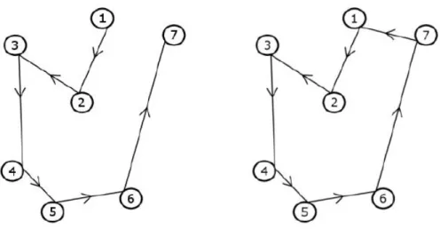
The Sequential Ordering Problem (SOP) is a well-known combinatorial problem defined on a graph. Given a graph G, with n vertices and m weighted directed edges, the SOP is the problem of finding the minimal cost Hamiltonian path from the start vertex to the terminal vertex, following precedence constraints on the vertex set [65]. In some literature, the SOP is associated to the TSPPC (or the asymmetric TSPPC), presented in the section 0, but it is different, in one characteristic. Both problems have precedence constraints in the vertex set. But, in the case of the SOP, there is only defined a fixed start and end node. While in the PCTSP, as already observed, it is required a closed tour where it is necessary one return to the start node. In the Figure 2 it is possible to observe the difference of two solutions for these problems. It is important to have in mind the precedence constraints presented in both solutions, having so the same sequence of nodes. Thus: (1) in the left for the SOP, with a fixed node and an end node, and (2) in the right for the PCATSP, with a closed tour [66][67].

(40)

Figure 2 - Examples of the SOP (right) and the TSPPC (left).

Thus, SOP is a generalization of the TSP, and so must be NP-Hard [68]. The scope of applications of this problematic is very wide, including, vehicle routing with pickup and deliveries, single-machine scheduling problems with set-up costs and precedence between jobs, among others [69].

A variation of SOP is the capacitated SOP. This problem adds the capacity constraint to the problem. Thus, a vehicle with a capacity Q and a precedence relation (

p,q

) is associated with a commodity that has a weight of

d

pq, needing so to be collected at

p

and delivered at

q

. Following the similarity between SOP and TSPPC stated previously, this variation of the problem is related to the Travelling Salesman Problem with Pickup and Deliveries [69].

There are some examples of different applications in literature. In [70], a metaheuristic Ant Colony Optimization algorithm that uses a local search to improve the overall performance of the ACO metaheuristic is developed. It is strongly based on an Ant Colony System and is a building heuristic in the sense that starts from node 0 and adds new nodes until all the nodes have been visited and the last node is reached, always according to the precedence constraints.

To see more applications and state of the art related to the SOP problematic, the reading of [68]is recommended.

(41)

3. D

YNAMIC

V

EHICLE

R

OUTING

3.1. O

UTLINE OF THE

D

YNAMIC

R

OUTING

P

ROBLEMS

The development of technologies lead to a model of different routing problems, dealing not only with static routing problems (as the examples already mentioned of the SPP and TSP), but also with dynamic routing problems. The dynamic routing problems arise due to the fact that static network optimization problems do not depend on the time and so, there are some time dependent parameters that are not considered [71].

Thus, a dynamic environment means that the information of the network may be changing during the execution of the algorithm. Moreover, following a dynamic environment, at each time, the choice of a route is based on the information then available [72]. In a dynamic routing problem, what may be the ‘best route’ for one to follow, may or not be the best, for the same entity, in a different time instant, due to the network information updates.

The Figure and Figure illustrate a possible scenario in a dynamic routing problem. Initially (Figure ), at time t0, the best route for a vehicle with characteristics x1, is starting

in the node ‘S’, following the sequence demonstrated in the Figure and turning back to ‘S’. The same vehicle (with characteristics x1), at the time t1 will have a different best route,

because the arc connecting the nodes ‘1’ and ‘2’ is unable to be traversed, due to some certain event (Figure ). Therefore, for the same vehicle and network, the assigned the route is different depending on the time.

(42)

Thus, in the dynamic routing problems there are certain events which may change the network and consequently change the transportation process [13]:

1. New Requests: If it is necessary to visit a new location closed to a planned location, (in a fixed time windows and/or other specified attributes), an adaptation of the tour may be necessary to include this new request.

2. Changes in request attributes: The attributes of each location may be different (requesting a different amount of goods, changing the time window, etc.). Therefore, it will be necessary to rearrange the previous tour, perhaps altering the path of the route, or altering some fleet characteristics.

3. Traffic Congestion and blocked roads: The traffic jam in the roads increase their travel times or can provoke a complete blockage of the affected roads. When this happens, reassigning the vehicles to non-congested roads, or allocating the requests to other vehicles may be necessary.

4. Vehicle disturbances: When a partial or complete deficiency on the vehicle exists, due to an accident or other possible scenario, the routing plan may be rearranged, assigning other vehicles to the requests of the incapacitated one.

A great different between the static and the dynamic routing problems is the objective function. In the static routing problems, usually the objective function tries to minimize the route cost. The dynamic routing problems introduce different scenarios, like service level, throughput time, or revenue maximization [73]. In real-time dynamic routing problems, the objective is sometimes the aggregate of several objectives, combining different measures [74].

Alan Larsen[75], proposes a framework, dividing the dynamic routing problems, depending on their degree of dynamism. The Weakly Dynamic Systems are problems in which the grater part of the information is known in advance, that is, at the time of the tours’ construction. The reacting time is considerably longer when compared with others and the tradicional way of solving this problem is to adapting static procedures. Thus, a static routing problem is solved every time an update on the network happens. The Strongly Dynamic Systems are characterized by the fast change of data, and by the urgency of requests received. As examples of this systems, are the emergency services (such as police,

(43)

fire department and ambulance), and the taxi cabs, in which only a few “customers” are known beforehand. Therefore, in such problems, the reaction time is of great importance.

With this necessity of updated information, dynamic routing problems usually involve more elements than the static routing problems, increasing so the complexity of their decisions and introducing new challenges while judging the merit of a given route plan [73] [76].

If a problem is dynamic, it can also be stochastic or deterministic [77][74]. In a deterministic and dynamic problem, part or all the information is unknown in advance and depend on time, being revealed during the design or execution of the routes, per example. For this problem, typically is necessary to have technological support, for example cellphones, or global positioning systems (GPS), for real-time communication between the vehicle and the central depot[73]. One example of a deterministic and dynamic problem is the one presented by Daskin [78]. In this problem, a TSP in a time dependent network is addressed. The time dependent TSP (TDTSP) is a generalization of the regular TSP, in which the travel time between two customers or between a customer and the depot depends on the distance between them, but also depends on the time of the day. Here, a Mixed Integer Linear Programing (MILP) formulation is presented, and the results are reported.

In a stochastic and dynamic problem, the uncertain data is represented by a stochastic process. Therefore, the unknown data is a collection of random variables, being so travel times, unknown demands and/or the existence of customers. The data are so gradually revealed during the operational interval, making so that they are not constructed beforehand [75]. One example of this type of problems is the case of the Dynamic Traveling Repairman Problem [79].

In addition to the examples previously presented, one of the most known routing problems in a dynamic network is the dynamic shortest path problem.

3.2. D

YNAMIC

S

HORTEST

P

ATH

P

ROBLEM

The dynamic shortest path problem is the generalization of the static SPP, already explained, where the characteristics of the network may change overtime.

(44)

Dynamic shortest path problems are computed in a time-dependent network, instead of a static network as in the static version of the SPP. Thus, a time-dependent Graph is defined as G=(V,E,T), where V is the set of nodes and E is the set of arcs representing the network segments, each one connecting two nodes. For every arc

e=(v

i

,v

j

)

∈ E

, and

v

i≠

v

j, there is a cost function

c

vi,vj(t), where

t

is the time variable in time domain T. This

cost function represents the travel time from

v

i to

v

j starting that arc in the time

t

[80].

Considering that a cost of one (or more) arcs may change during the calculations, the dynamic shortest path problem is to compute the shortest path between one to all the other nodes, or between all the pairs of nodes present in the network. Thus, the dynamic SPP deals with non-fixed arc costs [81].

Dynamic SPP can be further divided into two types, depending on how the time is treated [82]: discrete and continuous. In the discrete type, the time variable is modeled as a set of integers, while in the continuous, the time variable is treated as real numbers. Depending on the type of how the time is treated, the cost function can also be continuous in time, or discrete, whose domain and range are integers [83]. Therefore, dynamic SPP is more about fastest path than shortest path per se. Typically, the objective is to find the fastest path from one node to another, which may not be the shortest one in terms of distance. However, the time of traversing an arc is generally directly proportional to the distance of that arc.

The network can be also FIFO (first in, first out) or non-FIFO. If the condition FIFO holds, no one can depart later at the beginning of one or more arcs and arrive earlier. On the other hand, when the network is non-FIFO, it is possible for an entity to depart later and arrive earlier at the destination. The difference between the former networks lies on the travel functions of the arcs. If the functions are constant or increasing with time, means that the network is FIFO. If there is travel functions that are decreasing with time, the network is non-FIFO [80].

One practical example of such networks can be given by considering a link composed of two physical channels, one being faster than the other. If the policy is to send a message over the first available channel, then a message sent over the slower one may

(45)

arrive later than another message sent later in the fast channel, meaning that messages arrive in non-FIFO order [83].

These different types of networks bring many implications, such as, if waiting at nodes is possible or not, or if the time of the departure is restricted or unrestricted, etc. For example, if the network is non-FIFO, sometimes it may be preferable to wait a certain amount of time in the node, before entering in one arc. One other example can be the system entering time. This time is the time that the entity starts its route. If this time is restricted means that the entity must enter the system in a fixed time. On the other hand, the entity can have an allowed interval of time before entering the system. Such conditions will have impact on the solution of the shortest path.

An illustration of the dynamic shortest path problem is given in [84] and can be observed in the Figure 3. In this case, it is possible to state that, the edge ‘e’, has a time dependent cost. Therefore, when computing the shortest path from the source, ‘s’, to the destination, ‘d’, the shortest path and cost will depend on the time of the departure. The graph presented in the Figure 3 shows an example of a non-FIFO network.

Figure 3 - Example of a time dependent shortest path.

In the dynamic version of the SPP, the algorithms can also compute not only the shortest path from one-to-all given a departure time, but also from all-to-all for all departure times. As happens in the static version, this problem can be turned into the fastest path problem, least cost path problem, planning, etc. [82].

Compared to the static SPP, the literature in this problem is surprisingly much more limited. In the study of Cook and Halsey [85], a dynamic Programming algorithm is developed to address the dynamic SPP. In 1969, Dreyfus [86], is the first to address the time dependent shortest path with a generalization of the well-known Dijkstra’s algorithm.

(46)

In this generalization, waiting times at nodes were not allowed. It was proved [87], later, that this generalization is only valid if the network satisfies the FIFO conditions. On the other hand, the time-dependent cost functions of the arcs are usually difficult to be forecasted, thus the link travel times are typically described by random variables.

In [88], a study of the complexity of shortest paths in time-dependent graphs is outlined.

Besides routing, there are an enormous variety of problems were a dynamic modeling may be addressed. Among them are Design of a service network, Repositioning of empty vehicles to anticipate future demands, Production and Inventory Management, Facility planning and design, etc.[77].

Previously, four types of events with most impact in the dynamic routing problems were addressed and explained. The traffic jam was one of them and is mentioned as being one of the principal events in dynamic routing problems and is widely studied in literature.

3.3. T

RAFFIC

A

SSIGNMENT

3.3.1. O

VERVIEW

Since the early 1990’s, road traffic has been increasing and causing congestion, delays, accidents, and environmental problems, almost in all large cities [89] [90].

Besides this, congestion also results in a massive delay for the vehicles due to the fact that the time of traversing a road is unpredictably higher whenever congestion is present [91]. Therefore, traffic congestion is a noteworthy problem, and the reduction of the congestion a major challenge [92]. All the costs caused by the traffic can be reduced or even eliminated, by using the transportation systems efficiently. In literature, there are several strategies to avoid traffic congestion, depending on the problem, such as selecting alternative routes, changing the customer-vehicle assignment, among others [93].

To achieve an efficient way to organize the transportation system, the traffic (or transportation) planning problematic can be addressed [18]. The Traffic Planning can be divided into several processes [94], having in consideration goal definition, collection of

(47)

data, travel forecasting, among others, which are analyzed separately, and often in a predefined sequence.

In what this study concerns, one of the most important processes in Traffic Planning is the so-called Traffic Assignment. The Traffic Assignment is the part of traffic planning that determines traffic loadings on arcs and paths of the road network of interest in a static or dynamic environment [95]. The difference between static and dynamic is, as stated above, that a static approach, by definition, cannot reflect any variation in the traffic flows and any change in the transportation conditions, over time [96].

Therefore, succinctly, the Traffic Assignment Problem (TAP) is stated as follows [97]: Given a directed graph G, and a matrix of tours, containing the number of travelers from an origin location to a given destination in G, the TAP consists in determining a flow assignment on the links of G which satisfies the demand for each pair origin-destination (O-D) and minimizes each traveler’s time.

The major aims of TAP are the outlined above [98]: 1. Estimate the volume of traffic on the links.

2. Estimate inter zonal travel cost.

3. Analyze the travel pattern of each origin destination pair.

4. To identify congested links and to collect traffic data useful for the design of the transportation transport system.

The output of the TAP depends on the complexity of the application, but always give an estimate of the traffic volumes and the corresponding travel times or costs on each link of the transportation network. In a more sophisticated technique, the directional turning movements at intersections and route flows may be included to the assignment of traffic [94].

3.3.2. A

LL

-

OR

-N

OTHING

A

SSIGNMENT

One of the first heuristics to address the TAP was the all-or-nothing technique. This technique consists in the basic procedure of assigning all the traffic to the route with

(48)

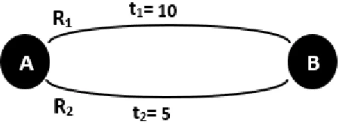
minimum traversing time [99]. In the Figure 4, there are two different routes, R1 and R2,

for reaching ‘B’ from ‘A’. Therefore, suppose that an amount of flow (vehicles),

x

, must be assigned to the origin-destination pair A-B, that is, starting in ‘A’ and traveling to ‘B’.

Figure 4 - Two routes example for the All or Nothing Assignment.

It is possible to observe in the Figure 4 that the cost (time) of traversing each route does not depend on the flow in the route, having then a constant cost. In the all-or-nothing procedure, all the amount of flow is assigned to R2, being that route the one of minimum

cost, regardless of x.

It is notable that this technique considers a highly unnatural assumption, that the travel cost is independent of the amount of flow present in the links. If, p. e., there are two alternative routes with a nearly cost, the assignment is always made to the minimum cost route [94].

Moreover, the assigning is made whether or not there is adequate capacity or heavy congestion on the links of the network. Despite this, this procedure may be efficient if the amount of flow to be assigned is low and/or if there are many alternative routes with an accentuated difference in the costs. It may also act as a building block for other models of traffic assignment [98].

This assignment can be made using only a TSP or a SPP instance (depending if there are more than a location to visit or not). Therefore, all the traffic is assigned to that route.

3.3.3. L

INK

C

OST

F

UNCTIONS

The results of the all-or-nothing technique are very unrealistic, as stated above. To introduce the concept of congestion, it is necessary to have algorithms considering that