MORTGAGE VALUATION
A Quasi-Closed Form Solution
Cristina Viegas
Faculdade de Economia and CASEE Universidade do Algarve
José Azevedo-Pereira
Instituto Superior de Economia e Gestão Universidade Técnica de Lisboa
MORTGAGE VALUATION: A QUASI-CLOSED FORM SOLUTION ABSTRACT
The main objective of this study consists in developing a quasi-analytical solution for the valuation of commercial mortgages. We consider the existence of a single source of risk - the risk of defaulting on a mortgage - and therefore, the existence of a single state variable - the value of the mortgaged property. The value of the mortgage corresponds to the present value of the future payments on the loan, minus the value of the embedded American default option. The major difficulty in designing such a model consists in calculating the value of this option, since for that purpose it is necessary to determine the lowest property price below which it must be immediately exercised, i.e. the critical value of the property.
Under such a framework, the partial differential equation for the value of the default option is that presented in Black and Scholes (1973). The boundary conditions applicable to the value of the default option are naturally different, given the possibility of early default. To obtain a quasi-closed form solution, instead of continuous time framework, a discrete time setting is considered for the differential equation - the “Method of Lines”. The partial differential equation is transformed into an ordinary non-homogenous differential equation, replacing the derivative of the function [price of the option in relation to time] with a finite difference, and keeping the derivatives of the mortgaged property unchanged. In order to improve the performance of the model, Richardson’s extrapolation is applied, allowing for the increase in the speed of convergence of the model results towards reasonable values.
As compared to the alternative numerical valuation techniques, the proposed quasi-closed form solution provides much quicker mortgage valuation results and enhances the ability to perform the corresponding sensitivity analysis. The current work constitutes one of the first attempts to address the development of analytical solutions to mortgage valuation, using contingent claims analysis.
1. Introduction
Contingent claims mortgage valuation models tend to assume that the main drivers for the value of these financial assets are the risks of prepayment and default. These sources of risk are normally modelled through the consideration of two stochastic variables: the interest rate and the value of the mortgaged property.
The possibilities held by the borrower to end the respective loan, either by way of prepayment or by way of default, represent sources of uncertainty that are not easy to model appropriately. The decision of the borrower is influenced by the future evolution of both interest rates and prices of the mortgaged property. The prepayment option embedded in a mortgage is equivalent to an American call option on a bond whose cash flows are equivalent to the outstanding payments inherent in the mortgage loan. In turn, the default option may be understood as an American put option, whose underlying asset is the mortgaged property1.
The contingent claims valuation models that take into consideration both mortgage options tend to allow for a good understanding of the characteristics and components of mortgage contracts. This is important not only academically, but also for its practical implications, since the pricing of assets may improve as a result of different investment banks progressively adopting these types of models.
In the most cases, the specialist literature has presented only numeric solutions for this type of evaluation. In order to obtain these solutions, complex calculation techniques are required, which means the process becomes overly slow and expensive.
1 It could also be seen, probably even more aptly, as a European compound option i.e. as a series of European put options with payments made on each of the due dates inherent in the loan (see, for example, Kau, Keenan, Muller and Epperson, 1995, and Azevedo-Pereira, Newton and Paxson, 2002, 2003).
In this area of research, an aspect that has still not been explored much is the development of closed form solutions for valuation of mortgage assets2. The mathematical complexity that derives from the simultaneous consideration of two American options has, up to now, impeded the development of efficient valuation models.
With the aim of making a contribution towards surpassing these difficulties, the main objective of this study is the development of a quasi-closed form solution that will allow the valuation of commercial mortgages. To make the modelling possible, a simplifying assumption is made: given the specific characteristics inherent to commercial mortgages, we do not take into consideration the prepayment option. Consequently, interest rates are not regarded as stochastic.
Under these assumptions, the value of the mortgage will correspond to the present value of the future payments minus the value of the default option. The present value of future payments is obtained by applying the concept of the present value of an annuity, since the interest rate is not stochastic. The value of the default option is determined using the principles that normally underlie the valuation of American put options.
Following this approach, the valuation of a commercial mortgage starts with the definition of the stochastic process used to characterize the behaviour of the stochastic variable considered in the model: the value of the mortgaged property. The most frequently used approach is that used by Black and Scholes (1973) and Merton (1973) for modelling the price of a European call option on a stock.
The next step consists of obtaining the partial differential equation for the value of the default option. This equation is, once more, that presented by Black and Scholes (1973). However, the boundary conditions applicable to the value of the default option are
2
Two exceptions are Collin-Dufresne and Harding (1999) - that proposes a closed form solution for fixed rate residential mortgages, using a single variable, the short-term interest rate – and Sharp, Newton and Duck (2006) that use singular perturbation theory to develop a closed-form solution for the value of a mortgage when both default and prepayment are included.
naturally different. The difference derives from the possible early exercise of the default option held by the borrower. In this sense, the main difficulty in designing the model lies in calculating the critical value of the property, i.e. the price level below which the option should be immediately exercised.
Considering the income of the mortgaged property as proportional to its value, a commercial mortgage valuation model is developed for which it is possible to derive a quasi-closed form solution.
The outline for this paper is as follows. Section 1 introduced the work. Section 2 describes the main assumptions underlying the mortgage valuation model and presents the stochastic processes followed by corresponding variables, the general partial differential equation and the corresponding options held by the borrower. It develops the commercial mortgage valuation model and presents its quasi-closed form solution. Some of the model limitations are identified. In section 3, the formulae derived during the course of the work are verified and validated via graphical and numerical analysis. Finally, the conclusion is presented, including suggestions for future developments.
2. The Mortgage Valuation Model
2.1. General Formulation of the Contingent Claims Mortgage Valuation Model
Some contingent claims mortgage valuation models include both risk factors inherent in a mortgage contract whilst others limit themselves to either the default or the prepayment option. This work uses a single variable, the value of the mortgaged property, B .
The stochastic process followed by the value of the property is identical to the process used by Black and Scholes (1973) and Merton (1973):
(
b)
Bdt BBdzBdB= α− +σ (1)
Where: ≡
α Instantaneous expected return on property ≡
b Continuous rate of property payout ≡
B
σ Instantaneous standard deviation ≡
B
z Standard Wiener process
Works such as Cunningham and Hendershott (1984), Epperson et al. (1985), Kau et al. (1987, 1990, 1992, 1993a, 1993b, 1995), Titman and Torous (1989), Schwartz and Torous (1992), Deng (1997), Yang et al. (1998), Hilliard et al. (1998), Ciochetti and Vandell (1999), Azevedo-Pereira et al. (2000, 2002, 2003), Downing et al. (2003), Sharp et al. (2006) are mortgage valuation studies in which (1) is used to characterise the value of a house or property.
After the presentation of the stochastic processes followed by the variable, the next step consists of deriving the partial differential equation for the value of a commercial mortgage, V, considering that there are no arbitrage opportunities. This equation results from the dynamics of the variable underlying the model, the value of the property.
(
)
(
) ( )
(
)
(
)
2 2 2 2 , , 1 , , 0 2 B V B V B V B r b B B rV B B B τ τ τ σ τ τ ∂ ∂ ∂ − + − + − = ∂ ∂ ∂ (2)This general equation allows the valuation of financial derivatives when the underlying variable follows the previously defined stochastic processes. The difference in valuation
formulae, for different financial assets, resides in the initial, final, and boundary conditions to be applied according to each concrete case.
2.2. The Model to Be Developed in this Work
2.2.1. General Characteristics
The current study is strictly focused on the analysis and valuation of a commercial mortgage with a default option. This sort of framework is in concordance with other work already undertaken in this area, such as Titman and Torous (1989). According to these authors, some types of commercial mortgages do not allow for the prepayment of the loan prior to its maturity. In effect, the institutional characteristics tend to make that postulation more reasonable in relation to commercial mortgages than in relation to residential mortgages.
Under these circumstances, the value of the mortgage corresponds to the value of a financial asset whose only source of risk derives from the possibility of borrower default.
Kau and Keenan (1999) state that it is possible to find analytic solutions for mortgage valuation models that consider the risk of default, if a reduced form of (2) - in which time is not taken into consideration – is used. To justify the removal of the time period from the equation, those authors propose studying the value of a perpetual mortgage with a fixed rate.
Following on from that study, the model here developed assumes that interest rates are constant and that prepayment is not allowed. However, contrary to what was established by Kau and Keenan (1999), the time period is not eliminated from the differential equation, which creates the possibility of evaluating a mortgage with a finite maturity.
In this context, the value of the mortgage is given by the following formula:
(
B)
A( )
P(
B)
In this equation, A
( )
τ equals the present value, in continuous time, of the future mortgage instalments:( )
− = − r e C A rτ τ 1 (4)Where, C, represents the annual value of the (fixed) instalment; r , the interest rate; and
τ, the number of years remaining until the maturity of the mortgage.
The other component of (3), P ,
(
τ B)
, equals the value of an American put option whose underlying asset is the value of the mortgaged property, B. The major challenge regarding the solution of (3) comes from this part of the equation. The literature presents numerous studies on the valuation of American puts, but for only a few particular cases is it possible to find analytic or quasi-analytic solutions. The problem becomes still more complicated when the underlying asset pays dividends. Unfortunately, that is the case modelled here, since properties provide revenue. In effect, the model assumes the existence of a revenue rate, b, proportional to the value of the property, and similar to that included in (1).2.2.2. The Default Option
At any moment in time, a borrower that defaults on mortgage instalments will lose his property. Consequently, a mortgage contract is equivalent to a American put option whose underlying asset is the value of the property and whose strike price is given by the present value of future instalments.
The value of this option is given by Black and Scholes (1973) partial differential equation:
(
)
(
)( )
(
)
(
)
0 , , 2 1 , , 2 2 2 2 = − ∂ ∂ + − ∂ ∂ + ∂ ∂ − rP B B B P B B b r B B P B P B τ τ σ τ τ τ (5)For the valuation of a mortgage default option, this equation is subject to the following boundary conditions:
(
,)
0 lim = ∞ → P Bτ B (6)(
Bτ)
A( )
τ B( )
τ P B B→ , = − lim (7)(
)
1 , lim =− ∂ ∂ → B B P B B τ (8)where B is the critical value of the property.
This is a completely borrower controlled (endogenous) default, based on the borrower’s expected price volatility.
As previously mentioned, obtaining a closed solution for this problem is a complex task. In spite of some advances made in the last few years, it has not been possible to arrive at a consensual analytical solution.
The possibility of early default constitutes the main obstacle in determining a closed solution. Therefore, most of the works that present solutions for pricing these options use numerical methods to determine the critical price of the underlying asset. For example, studies such as Kim (1990), Jacka (1991) and Carr et al. (1992) consider that the value of the American option is equal to the value of a European option3, increased by a premium given by the present value of the gains induced by early termination. This premium is obtained though an integral equation, whose exercise boundary is determined by a reversive numerical procedure.
In turn, studies such as those by Geske and Johnson (1984), Bunch and Johnson (1992), Ho et al. (1994), Huang et al. (1996), and Lee and Paxson (2003) develop an analytical approximation for the price of an American put option by means of calculating the value of a set of options with discrete exercise dates. The main difference between these studies lies in the number and exercise dates of the options used for calculating the value of the American put, as well as in the extrapolation method4 used with the intention of obtaining a satisfactory approximation for the value of the option. However, these works also do not determine analytically the critical value of the underlying asset. Recently, Zhu (2006) derived a closed-form solution for the value of the American put and its optimal exercise boundary, which is based on the homotopy-analysis method.
One of the improvements introduced in this field during the last decade consists of using the ‘Method of Lines’. The MOL was used in option valuation frameworks by Carr and Faguet (1996) and by Meyer and J. van der Hoek (1997). The first of these works utilised the method to generate explicit formulae for the approximate value of an American option and the corresponding critical exercise price. The second dealt with how the method might be used in the study and numerical valuation of American options and also as a means of determining the early exercise boundary.
Apart from Carr and Faguet (1996), another reference in the field of analytic solutions for American put options is Carr (1998). This article conceives time as random, considering that it follows an Erlang or gamma distribution. Although the methods used to reach quasi-analytic solutions were different in Carr (1998) and Carr and Faguet (1996), the results obtained in both articles were the same.
The present work follows Carr and Faguet (1996) and uses the MOL to pursue the outlined goal of obtaining a quasi-closed solution for mortgage valuation.
3
The value of the European option is obtained according to the formula given by Black and Scholes (1973).
2.2.3. Commercial Mortgage Valuation Model: a Quasi-Closed Form Solution
In mortgage valuation models, application of the MOL has implications regarding the way in which the present value of future loan instalments is calculated. Additionally, it has also repercussions concerning the differential equation for the value of the embedded default option.
As far as the present value of future instalments is concerned, instead of using a continuous time formulation, it is necessary to use the corresponding formulae in discrete time.
Based on this modification:
+ − = n n r r C A τ 1 1 1 (9)
In this equation, C , the annual value of the continuous instalments, is substituted by n
constant discrete instalments whose value is
n
Cτ . When the MOL is applied to calculate the value of the default option, the number of constant instalments should coincide with the number of intervals in which the time to maturity of the contract is subdivided.
In determining the value of the default option, following the approach proposed by Carr and Faguet (1996) for the valuation of American options, the Method of Lines (MOL) is applied. This means that the time derivative of the function [price of the option in relation to time] is replaced by a finite difference. The approximation error tends to reduce as the 4 Some use linear extrapolation, whil
size of the time increment used in the MOL is reduced. In this way, to obtain a good approximation to the value of the option, it would be convenient to consider time as divided into a number of intervals tending towards infinity. However, a higher number of time intervals implies a significant increase in mathematical computation. Therefore, there is a tendency to use a relatively small number of time intervals5, usually four. Afterwards, Richardson’s extrapolation6 is normally applied to accelerate the convergence of results towards values closer to reality. Richardson’s extrapolation is a technique that allows an accelerated convergence of results towards the reference values, despite the fact that time is considered as being broken down into a relatively lower number of sub-periods.
With the application of this method, the differential equation given in (5), takes on the following form, for B ≥Bk:
( )
( )( )
( )( )
( )( )
( )( )
( )( )
n k k k k B k B P B P B rP B B P B B b r B B P τ σ 2 2 2 2 1 2 1 − − = − ∂ ∂ + − ∂ ∂ (10)To calculate P( )k
( )
B it is necessary to determine in advance the expression for P(k 1−)( )
B , which implies that this equation should be solved for k=1,2,3,47. This equation is somewhat simplified in relation to equation (5), since the price of the option becomes a function of a single variable, the value of the mortgaged property. Given this alteration, the general expression for the value of the mortgage contract is the following:
5 Considering the period to maturity of the contract as being divided into four time intervals gives a most acceptable estimate for the value of an American put option. In mortgage valuation, the same rationale is applied, since the valuation of a default option is conceptually similar to the valuation of an American put option.
6
For an introduction to the use of this type of extrapolation, see Carr (1998). 7
k is equal to the number of sub-periods in relation to the total number of time intervals, n=4, considered in the model. In this way, the expression of the mortgage value for k4τ time periods is calculated with
4 , 3 , 2 , 1 = k .
( )
( )
P( )( )
B n r r C B V k n − k + − = τ 1 1 1 (11)where P( )k
( )
B corresponds to the value of the option that complies with equation (10). In accordance with what was previously stated, n , the number of time intervals, should beequal to 4.
In turn, equation (11) is valid for values that comply with the following restrictions:
( )
( )
+ − = ∞ → n k B n r r C B V τ 1 1 1 lim (12) ( )( )
k k B B kV B B = → lim (13) ( )( )
1 lim = ∂ ∂ → B B V k B B k (14)Condition (12) stipulates that, when the price of the property tends towards infinity, the value of the mortgage coincides with the present value of the future loan instalments. In this situation the value of the default option is null. The delimitation of the lowest value for the mortgage price interval is given by equations (13) and (14). These restrictions impose the value of the mortgage contract to be equal to the price of the property, when this price tends towards its critical level, B . Consequently, fork B ≤Bk, the borrower does not fulfil his financial obligations and loses the property. In accordance with these conditions, the value of the mortgaged asset, before the maturity of the contract, should comply with the following relationship: V( )k
( )
B ≤ . BThe solution of (11), subject to restrictions (12), (13), and (14), leads to a general solution for the mortgage value, that varies in accordance with the interval considered for the price of the property. The period to maturity is divided into n time intervals, n = 1,2,3,4. The formulae presented correspond to the value of the mortgage whose term until maturity is equal to n kτ with k=1,2,3,4 and k ≤ . n Therefore, forB ≥B1 8
,k=1,2,3,4 and n=1,2,3,4 the mortgage value is given by:
[ ]( )
( )
( )
( )
( )
( )
( )
+ + + + + + + + + − = − − − − + + − ≥ 2 3 2 5 2 2 1 3 2 2 2 4 2 3 6 3 3 4 2 2 2 2 2 1 2 2 2 ln ln 9 ln 30 30 3 2 ln 2 ln 2 -1 1 1 n n n n k n n k n n k k b r n k B B B B B a n B a n B na a B r n r C B V n ρ ρ τ σ ρ σ τ ρ σ τ ρ τσ ρ ρ ρ τσ τ τσ ρ τσ τ τ ifB ≥B1 (15) where:ak-i = 0 for k – i < 0 and i = 1,2,3.
For B ≤Bk 9 and k=1,2,3,4, the mortgage value becomes:
8
1
B corresponds to the critical value of the property over a period of possession of the contract equal to
n
τ
.
[
]
( )( )
B B VB B kk =
≤ if B ≤Bk (16)
In relation to the area where B2≤B≤B1 , for k=2,3,4 and n=2,3,4 the value is given by: [ ]( )
( )
( )
( )
[
( )
( )
− + − + − + + + + + + − + − + + − = − − − − + + + − − − − − + + − − − ≤ ≤ 2 2 3 2 2 2 1 2 2 2 1 2 2 3 2 2 2 1 2 2 2 1 1 2 ln 2 ln 2 1 2 ln 2 ln 2 1 1 1 1 1 1 2 2 2 2 1 2 n n k n n k k b r k n n k n n k k b r k k n k B B B B z n B nz z B n b B B y n B y y B n r r n r n r C B V n n ρ τσ ρ ρ ρ τσ τ ρ τσ ρ ρ ρ τσ τ τ τ τσ ρ τσ τ τ τσ ρ τσ τ τ where: 0 = −i ky and zk−i=0 for k− i≤0 and i=2,3.
In turn, for B3≤B≤B2 , k=3,4 and n=3,4, the mortgage value is given by:
if B2≤B≤B1
(17)
[ ]( )
( )
( )
( )
+ + − + + − + − + − + + − = − − − + + − − − − + + + − − − ≤ ≤ n n k k b r k n n k k b r k k n k B B B B nx x B n b B B nw w B n r r n r n r C B V n n ρ ρ τσ τ ρ ρ τσ τ τ τ τσ ρ τσ τ τ τσ ρ τσ τ τ ln 2 1 ln 2 1 1 1 1 1 1 2 3 2 2 2 2 2 2 3 2 2 2 2 2 2 2 2 2 2 2 3 where: 0 = −i kw and xk−i =0 for k− i≤0 and i=3.
For B4≤B≤B3 , k=4 and n=4, the mortgage value becomes:
[ ]( )
( )
1 1 1 1 1 1 1 2 2 2 2 3 4 2 2 2 1 2 2 2 1 τσ ρ τσ τ τ τσ ρ τσ τ τ τ τ τ τ n n r b b r n k B B B B v B u n b B n r r n r n r C B V − + + − + + + − ≤ ≤ − − + + + − + + − =Regarding equations (15), (16), (17), (18), and (19):
(
2)
2 2(
2)
2 8 2 4 2 τ τσ τ σ σ ρn= r + + b − r+b+ + nThese different expressions for the value of the mortgage contain a set of parameters whose value is determined by the solution of a system of equations. It is necessary to
if B3≤B≤B2 (18)
solve a set of equations that must be verified by the different mortgage value expressions. Thus, we arrive at:
For k=1, n=1,2,3,4and B =B1:
[
]
( )( )
B V[
]
( )( )
B V B B k k B B≥1 = ≤1 (20)[
]
( )( )
1 1 = ∂ ∂ ≥ B B VB B k For k=2,3,4 , n=2,3,4and B =Bk:[
]
( )( )
B V[
]
( )( )
B V B B B k k B B≤ k = k≤ ≤ k−1 (21) For k=2,3,4, n=2,3,4andB =B1:[
]
( )( )
B V[
]
( )( )
B VB B k B B B k 1 2 1 ≤ ≤ ≥ = (22)[
]
( )( )
[
]
( )( )
B B V B B V B B B k k B B ∂ ∂ = ∂ ∂ ≥ ≤ ≤ 1 2 1 For k=3,4 , and n=3,4 B =B2:[
]
( )( )
B V[
]
( )( )
B VB B B k B B B k 1 2 2 3≤ ≤ = ≤ ≤ (23)[
]
( )( )
[
]
( )( )
B B V B B V B B B k k B B B ∂ ∂ = ∂ ∂ ≤ ≤ ≤ ≤ 1 2 2 3 For k=4 and B =B3:[
]
( )( )
B V[
]
( )( )
B VB B B k B B B k 2 3 3 4≤ ≤ = ≤ ≤ (24)[
]
( )( )
[
]
( )( )
B B V B B V B B B k k B B B ∂ ∂ = ∂ ∂ ≤ ≤ ≤ ≤ 2 3 3 4For a numerical determination of the critical values B , for k B=Bk, k=2,3,4 and 4 , 3 , 2 =
n , a numerical solution10 for the following equation is required:
[
]
( )( )
1 1 = ∂ ∂ ≤ ≤ − B B VB B B k k k (25)The equations presented above allow for a quasi-closed form solution because the only equation which is not a closed form solution is the equation that determines the critical value of the property.
2.2.4. Applying Richardson’s Extrapolation to the Commercial Mortgage Valuation Model
Richardson’s extrapolation permits us to obtain a good estimate for the value of a function when continuous time is replaced by discrete time. Notwithstanding the fact that, in working out these formulae, the reference period is subdivided into a relatively small number of intervals - in this case four intervals - the results obtained are very close to those that would be obtained if time was to be considered as continuous.
Applying Richardson’s extrapolation to the mortgage valuation model results in a formula that allows for the calculation of both the extrapolated value of the mortgage,
( )
0 ˆV , and the critical price of the mortgaged property, Bˆ4
( )
0 .The extrapolated value of the mortgage is given algebraically as follows:
10
( )
V( )
τ V( )
τ V( )
τ V( )
τ V ˆ 6 1 ˆ 4 ˆ 2 27 ˆ 3 32 0 ˆ 2 3 4 − + − = (26)where the functions Vˆ
( )
τn , for n=1,2,3,4, correspond to the values obtained from the previously calculated functions, V( )k( )
B , for n= k=1,2,3,4.In turn, the extrapolated critical value of the mortgaged property is given by:
( )
( )
τ( )
τ( )
τ( )
τ 1 2 2 3 3 4 4 4 ˆ 6 1 ˆ 4 ˆ 2 27 ˆ 3 32 0 ˆ B B B B B = − + − (27)where Bˆk
( )
nτ corresponds to the value of B , for k n= k=1,2,3,4.The numerical results obtained through the application of this model are presented in the following section, as well as an analysis of mortgage price sensitivity in relation to the price of the mortgaged property. As noted, the results obtained using the model developed in this study are consistent with economic rationale.
3. Mortgage Valuation Model Results
This section presents and discusses, both graphically and numerically, the results obtained using the general commercial mortgage valuation model previously developed. It does so by taking into account a basic set of economic parameters, using standard assumptions taken from the literature11. The analysis is carried out by way of graphs representing the evolution of the value of the mortgage asset, as well as tables presenting the numerical values for the critical price and the value of the mortgage.
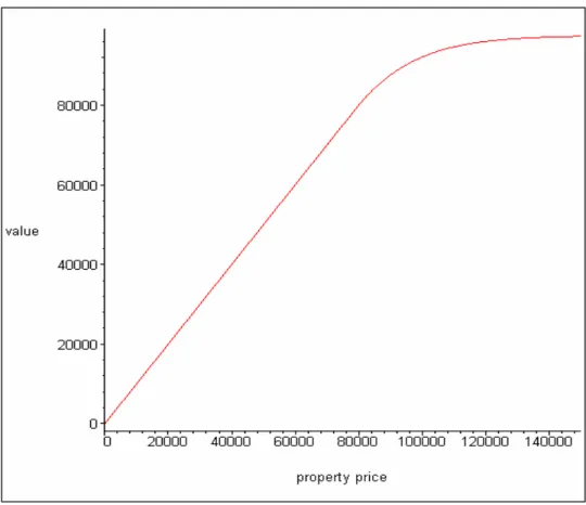
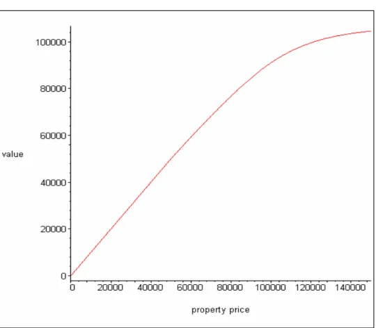
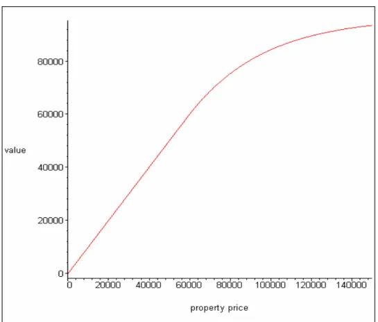
Figures 1 to 4 illustrate mortgage values as a function of the underlying property value. In these figures, the time to maturity is 3 years and the annual instalment is € 37 224. In Figures 1 to 3, the volatility of the property price is 15%, and in Figure 4 30%. Figures 1, 3 and 4 assume annual revenue yield is 5%, and Figure 2 assumes 10%. The interest rate in Figures 1, 2 and 3 is 7.5%, and 2.5% in Figure 4.
In all calculations, the period to maturity was subdivided into four time intervals that encompass five distinct functions, in accordance with each specific property price interval.
The graphical representation of mortgage value allows for a general conclusion: whenever the property price is above the critical level, positive variations in the property price imply a growth in the value of the mortgage, this value being lower than that of the property. However, when the property price is below the critical level, the value of the mortgage coincides with the value of the property.
All the graphs show that the line representing mortgage value as a function of property price has a positive slope, being divided into distinct zones: a default zone, for property values below the critical price, where the value of the mortgage coincides with the value of the property, represented graphically by a straight line with a slope of 1; a zone of contract compliance, for property values above the critical price, which is represented in the graphs by an increasing function with a decreasing growth rate. In every case the solution evolves smoothly across the state space.
The differences between the figures are due to the different values assumed for the model parameters. A comparison between Figures 1 and 2 shows that an increase in the annual rate of revenue induces a reduction in the critical price of the property, and consequently, a reduction in the value of the mortgage, for property prices above the critical price. The revenue is a dividend like feature whose increase will reduce the attraction of default.
Ceteris paribus, with higher revenue, a greater fall in property prices will be needed to
parameters remain unchanged, a fall in interest rates induces a reduction in the critical price of the property, and consequently, a reduction in the value of the mortgage, for property prices above the critical price. The value of the default option will increase, so the price will need to fall more to justify an immediate exercise. Regarding Figures 1 and 4, it can be observed that an increase in the volatility of property prices leads to a reduction in the critical price of the property and in the value of the mortgage. A rise in property price volatility will increase the value of the default option, which is a negative component of the mortgage value12. Immediate exercise will be less appealing and, consequently, the critical value will fall.
12
Figure 1. Commercial Mortgage Value as a Function of B
Values of parameters underlying the construction of this figure are as follows: n, the number of time intervals is 4; τ, the term remaining to maturity is 3 years; r, the interest rate is 0.075; σ , the volatility of the property price is 0.15; b, the annual rate of revenue is 0.05; C, the value of the fixed annual instalment is 37224; and,B4, the critical price of the property is 79082.
value
Figure 2. Commercial Mortgage Value as a Function of B
Values of parameters underlying the construction of this figure are as follows: n, the number of time intervals is 4; τ, the term remaining to maturity is 3 years; r, the interest rate is 0.075; σ , the volatility of the property price is 0.15; b, the annual rate of revenue is 0.10; C, the value of the fixed annual instalment is 37224; and,B4, the critical price of the property is 63064.
Figure 3. Commercial Mortgage Value as a Function of B
Values of parameters underlying the construction of this figure are as follows: n, the number of time intervals is 4; τ, the term remaining to maturity is 3 years; r, the interest rate is 0.025; σ , the volatility of the property price is 0.15; b, the annual rate of revenue is 0.05; C, the value of the fixed annual instalment is 37224; and,B4, the critical price of the property is 46869.
Figure 4. Commercial Mortgage Value as a Function of B
Values of parameters underlying the construction of this figure are as follows: n , the
number of time intervals is 4; τ, the term remaining to maturity is 3 years; r , the interest rate is 0.075; σ, the volatility of the property price is 0.30; b , the annual rate of revenue
is 0.05; C , the value of the fixed annual instalment is 37224; and,B , the critical price of 4
the property is 59243.
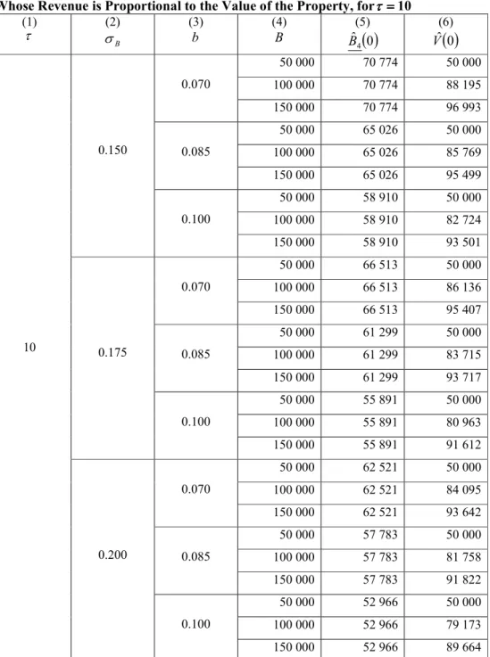
To end this section, two tables are presented with results for the critical price of the property and the value of the commercial mortgage obtained through application of the model proposed in this work. Columns (1), (2), (3), and (4) show different values for the parameters of the model, whilst columns (5) and (6) show the extrapolated values of the critical price, Bˆ4
( )
0 , and the value of the mortgage, Vˆ( )
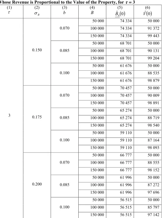
0 . All values were obtained through application of the model and then subjected to Richardson’s extrapolation.The difference between the two tables derives from the times to maturity and values of each fixed annual instalment considered. The value of the annual instalment was determined in order that the present value of the whole stream of future instalments, in continuous time, would reach an amount of (approximately) € 100000. It is shown that,
ceteris paribus, extending the time to maturity of the loan reduces the critical price and
the value of the mortgage, since the value of the default option tends to rise with an increase in the corresponding maturity. On the other hand, when the volatility is raised, the critical price comes down, reducing the default range of the contract, since once again the value of the option will increase.
Table 1. Values for Critical Price and for the Value of a Commercial Mortgage Whose Revenue is Proportional to the Value of the Property, forττττ ====10
(1) τ (2) B σ (3) b (4) B (5)
( )
0 ˆ 4 B (6)( )
0 ˆ V 50 000 70 774 50 000 100 000 70 774 88 195 0.070 150 000 70 774 96 993 50 000 65 026 50 000 100 000 65 026 85 769 0.085 150 000 65 026 95 499 50 000 58 910 50 000 100 000 58 910 82 724 0.150 0.100 150 000 58 910 93 501 50 000 66 513 50 000 100 000 66 513 86 136 0.070 150 000 66 513 95 407 50 000 61 299 50 000 100 000 61 299 83 715 0.085 150 000 61 299 93 717 50 000 55 891 50 000 100 000 55 891 80 963 0.175 0.100 150 000 55 891 91 612 50 000 62 521 50 000 100 000 62 521 84 095 0.070 150 000 62 521 93 642 50 000 57 783 50 000 100 000 57 783 81 758 0.085 150 000 57 783 91 822 50 000 52 966 50 000 100 000 52 966 79 173 10 0.200 0.100 150 000 52 966 89 664The values for the remaining parameters in the table are as follows: n , the number of time intervals is 4; C , the fixed annual instalment is 14 215; and, r , the interest rate is 0.075.
Table 2. Values for Critical Price and for the Value of a Commercial Mortgage Whose Revenue is Proportional to the Value of the Property, for ττττ====3
(1) τ (2) B σ (3) b (4) B (5)
( )
0 ˆ 4 B (6)( )
0 ˆ V 50 000 74 334 50 000 100 000 74 334 91 372 0.070 150 000 74 334 99 443 50 000 68 701 50 000 100 000 68 701 90 131 0.085 150 000 68 701 99 204 50 000 61 676 50 000 100 000 61 676 88 535 0.150 0.100 150 000 61 676 98 879 50 000 70 457 50 000 100 000 70 457 90 009 0.070 150 000 70 457 98 891 50 000 65 274 50 000 100 000 65 274 88 719 0.085 150 000 65 274 98 540 50 000 59 110 50 000 100 000 59 110 87 164 0.175 0.100 150 000 59 110 98 093 50 000 66 777 50 000 100 000 66 777 88 555 0.070 150 000 66 777 98 152 50 000 61 996 50 000 100 000 61 996 87 272 0.085 150 000 61 996 97 696 50 000 56 515 50 000 100 000 56 515 85 797 3 0.200 0.100 150 000 56 515 97 142The values for the remaining parameters in the table are as follows: n , the number of time intervals is 4; C , the fixed annual instalment is 37 224; and, r , the interest rate is 0.075.
The objective of this section was to test the viability of the model proposed in this work. Graphic and numeric analysis have shown that the results obtained, namely those analysing sensitivity of mortgage value in relation to property value, are consistent with economic intuition and evolve smoothly along the state space.
4. Conclusion
The substantial growth observed in commercial mortgage contracts during the last two decades justifies a greater academic effort in order to develop adequate valuation models. In the vast majority of cases, literature in this field has presented only numeric solutions. In order to obtain these numeric solutions, highly complex calculation techniques are required, which make the process overly slow and expensive. The main objective of this work is to make a contribution in a hitherto under-explored area of financial research: the development of a contingent claims commercial mortgage valuation model with a closed form solution.
The model developed in the present paper constitutes one of the first attempts to identify closed form solutions for commercial mortgage valuation. It is also a valid alternative to models proposed up to now in the specific field of commercial mortgage valuation. The corresponding results are much easier and quicker to find than the numerical solutions normally obtained in mortgage valuation models. Additionally, as can be inferred from the graphical representation of mortgage price sensitivity in relation to the value of the mortgaged property, these results make economic sense and evolve smoothly across the state space, evidencing the reasonability of the approach developed.
It is hoped that this study has contributed in some way towards advancing an area in which there has been little investigation, up to now. However, it is important to recognise that there is considerable room for further research. Following directly from our work, a significant improvement could result from the development of a general solution applicable independently of the number of periods used in the discretization process. Another, more ambitious improvement, would be the development of a model whose
final result is given by an analytic solution in continuous time. In this situation, it would not be necessary to apply Richardson’s extrapolation and the whole valuation procedure would become considerably more elegant.
Acknowledgements
The authors thank the referees for their valuable suggestions and remarks, which have improved the paper.
BIBLIOGRAPHY
Azevedo-Pereira, J. A., D.P. Newton and D.A. Paxson (2000) Numerical Solution of a Two State Variable Contingent Claims Mortgage Valuation Model, Portuguese Review of Financial Markets, 3, 1, 35-65.
Azevedo-Pereira, J. A., D.P. Newton and D.A. Paxson (2002) UK Fixed Rate Repayment Mortgage and Mortgage Indemnity Valuation, Real Estate Economics, 30, 2, 185-211.
Azevedo-Pereira, J. A., D.P. Newton and D.A. Paxson (2003) Fixed Rate Endowment Mortgage and Mortgage Indemnity Valuation, Journal of Real Estate Finance and Economics, 26, 2-3, 197-221.
Black, F. and M. Scholes (1973) The Pricing of Options and Corporate Liabilities,
Journal of Political Economy, 81, 3, 637-659.
Bunch, D. and H. E. Johnson (1992) A Simple and Numerically Efficient Valuation Method for American Puts Using a Modified Geske-Johnson Approach, Journal of Finance, 47, 809-816.
Carr, P. (1998) Randomization and the American Put, Review of Financial Studies, 11, 3,
597-626.
Carr, P. and D. Faguet (1996) Valuing Finite-Lived Options as Perpetual, Morgan Stanley, Working Paper.
Carr, P., R. Jarrow and R. Myneni (1992) Alternative Characterizations of American Put Options, Mathematical Finance, 2, 87-106.
Ciochetti, B.A. and K.D. Vandell (1999) The Performance of Commercial Mortgages,
Real Estate Economics, 27, 1, 27-61.
Collin-Dufresne, P. and J.P. Harding (1999) A Closed Form Formula for Valuing Mortgages, Journal of Real Estate Finance and Economics, 19, 2, 133-146.
Cunningham, D. and P.H. Hendershott (1984) Pricing FHA Mortgage Default Insurance,
Housing Finance Review, 3, 4, 383-392.
Deng, Y. (1997) Mortgage Termination: An Empirical Hazard Model with a Stochastic Term Structure, Journal of Real Estate Finance and Economics, 14, 3, 309-331.
Downing, C., R. Stanton and N.E. Wallace (2003) An Empirical Test of a Two-Factor Mortgage Valuation Model: How Much Do House Prices Matter?, Paper RPF-296, Research Program in Finance Working Papers.
Epperson, J.F., J.B. Kau, D.C. Keenan and W.J. Muller III (1985) Pricing Default Risk in Mortgages, Journal of AREUEA, 13, 3, 261-272.
Geske, R. and H. E. Johnson (1984) The American Put Valued Analytically, Journal of Finance, 39, 1511-1524.
Hilliard, J.E., J.B. Kau and V.C. Slawson (1998) Valuing Prepayment and Default in a Fixed-Rate Mortgage: A Bivariate Binomial Options Pricing Technique, Real Estate Economics, 26, 3, 431-468.
Ho, T. S., R.C. Stapleton and M.G. Subrahmanyam (1994) A Simple Technique for the Valuation and Hedging of American Options, Journal of Derivatives, 2, 52-66.
Huang, J., M. Subrahmanyam and G. Yu (1996) Pricing and Hedging American Options: A Recursive Integration Method, Review of Financial Studies, 9, 1, 277-300.
Jacka, S. D. (1991) Optimal Stopping and the American Put, Mathematical Finance, 1,
1-14.
Kau, J.B. and D. C. Keenan (1995) An Overview of the Option-Theoretic Pricing of Mortgages, Journal of Housing Research, 6, 2, 217-244.
Kau, J.B. and D.C. Keenan (1999) Patterns of Rational Default, Regional Science and Urban Economics, 29, 6, 765-785.
Kau, J.B., D.C. Keenan, W.J. Muller and J.F. Epperson (1987) The Valuation and Securitization of Commercial and Multifamily Mortgages, Journal of Banking and Finance, 11, 525-546.
Kau, J.B., D.C. Keenan, W.J. Muller and J.F. Epperson (1990) Pricing Commercial Mortgages and Their Mortgage-Backed Securities, Journal of Real Estate Finance and Economics, 3, 4, 333-356.
Kau, J.B., D.C. Keenan, W.J. Muller III and J.F. Epperson (1992) A Generalized Valuation Model for Fixed-Rate Residential Mortgages, Journal of Money, Credit and Banking, 24, 3, 279-299.
Kau, J.B., D.C. Keenan, W.J. Muller III and J.F. Epperson (1993a) Option Theory and Floating-Rate Securities with a Comparison of Adjustable and Fixed-Rate Securities,
Journal of Business, 66, 4, 595-618.
Kau, J.B., D.C. Keenan, W.J. Muller III and J.F. Epperson (1993b) An Option Based Pricing Model of Private Mortgage Insurance, Journal of Risk and Insurance, 60, 2,
Kau, J.B., D.C. Keenan, W.J. Muller III and J.F. Epperson (1995) The Valuation at Origination of Fixed Rate Mortgages with Default and Prepayment, Journal of Real Estate Finance and Economics, 11, 1, 5-39.
Kim, I.J. (1990) The Analytic Valuation of American Puts, Review of Financial Studies,
3, 4, 547-572.
Lee, J. and D.A. Paxson (2003) Confined Exponential Approximations for the Valuation of American Options, European Journal of Finance, 9, 1-26.
Merton, R.C. (1973) The Theory of Rational Option Pricing, Bell Journal of Economics and Management Science, 4, 1, 141-183.
Meyer, G.H. and J. van der Hoek (1997) The Valuation of American Options with the Method of Lines, Advances in Futures and Options Research, 9, 265-285.
Riddiough, T. J. and H.E. Thompson (1993) Commercial Mortgage Pricing with Unobservable Borrower Default Costs, Journal of AREUEA, 21, 3, 265-291.
Schwartz, E.S. and W.N. Torous (1992) Prepayment, Default, and the Valuation of Mortgage Pass-Through Securities, Journal of Business, 65, 2, 221-239.
Sharp, N.J., D.P. Newton and P.W. Duck (2006) An Improved Fixed-Rate Mortgage Valuation Methodology with Interacting Prepayment and Default Options, Journal of Real Estate Finance and Economics, to appear.
Titman, S. and W. Torous (1989) Valuing Commercial Mortgages: An Empirical Investigation of the Contingent-Claims Approach to Pricing Risky Debt, Journal of Finance, 44, 2, 345-373.
Yang, T. T., H. Buist and I.F. Megbolugbe (1998) An Analysis of the Ex Ante Probabilities of Mortgage Prepayment and Default, Real Estate Economics, 26,4,
651-676.
Zhu, song-Ping (2006) An Exact and Explicit Solution for the Valuation of American Put Options, Quantitative Finance, 6, 3, 229-242.