Intelligent system for associative pattern identification in data

M

ASTER

Management Information Systems

M

ASTER

´

S

F

INAL

W

ORK

P

ROJECT

I

NTELLIGENT SYSTEM FOR ASSOCIATIVE PATTERN

IDENTIFICATION IN DATA

N

ELSON

S

OUSA

M

ARQUES

M

ASTER

Management Information Systems

M

ASTER

´

S

F

INAL

W

ORK

Project

I

NTELLIGENT SYSTEM FOR ASSOCIATIVE PATTERN

IDENTIFICATION IN DATA

N

ELSON

S

OUSA

M

ARQUES

A

:

A

M

P

R

i

G

LOSSARY

DM – Data Mining

KDD – Knowledge Discovery in Databases MAE – Mean Absolute Error

MSE – Mean Squared Error MedAE – Median Absolute Error ARM – Association Rule Mining TID – Transaction identifier BFS – Breadth First Search DFS – Depth First Search

ii

A

BSTRACT

Nowadays, data mining is one of the biggest topics in organizations, being a field with many research provided from all the fields that complement it. Data mining changed the typical approach of data analysis providing several tools to analyse large amounts of data, where the aim is the creation of new insights about some topic.

The typical output that is provided for the analytical tools are based on the numerical results, where is displayed a group of important metrics for analysis. For many people statistics is a difficult task to be done, where the output that is given from the analytic tools can be complicated to understand. With this idea it was investigated the possibility of creation of a system that provides the creation some models to the users where is provided some guidelines about the most important values to take care for each model.

The goals of this project are the development of the knowledge about Data Mining, learn how to use Python to produce data analysis, verify the existent machine learning applied to data for Python and use some data mining techniques to create a small system for associative models.

The system is capable to perform a Linear Regression, a Logistic Regression, a Correlation Coefficient and an Association Rule Mining algorithm. For each method is provided an output that contains the numerical results of the method and it was produce some guidelines with general ideas, assumptions of each method and it is interpreted the most important statistical values to facilitate the understanding of all the methods. The system was developed in Python. Three methods were created are based on machine learning algorithms. The association rule mining algorithm was created from the beginning. The association rule mining algorithm developed was FP-growth. The system was ready to run in Linux.

KEYWORDS: Data Mining; Statistics; Machine Learning; Multiple Linear Regression;

Cross-validation; Logistic Regression; Association Rule Mining; FP-growth algorithm; Scikit-learn; Statsmodels; Python.

iii

R

ESUMO

Nos tempos de hoje data mining é um dos tópicos que maior relevo tem ganho dentro das organizações, sendo também objeto de grande pesquisa e desenvolvimento no meio académico. Data mining veio revolucionar as abordagens tradicionais de criação de modelos, trazendo para as organizações um imenso conjunto de novas formas e técnicas para esta tarefa, de onde se retira valor da tecnologia para facilitar a tarefa e aumentar a robustez e qualidade de modelos, com o objetivo de criar elucidações sobre os modelos formulados para os intérpretes.

Os resultados das ferramentas estatísticas são meramente baseados em valores onde toda a interpretação e compreensão do que está gerado passa pelo intérprete que está a analisar os seus resultados. Esta tarefa de compreensão é muitas vezes complicada por vários fatores sendo um dos quais o facto do intérprete não conseguir captar sobre os resultados o que é relevante para avaliar o modelo formulado, não conseguindo considerar se este é válido ou não o que, por consequência, poderá levar à utilização de modelos que podem ser descabidos e sem fundamento. Com esta ideia em consideração foi desenvolvido, em ambiente Linux, um pequeno sistema com algumas técnicas de data mining de carácter associativo. Neste sistema é gerado um relatório específico por cada modelo onde são analisados os fatores mais relevantes para a criação de modelos, guiando desta forma o intérprete para a decisão de validar e utilizar o modelo criado ou a rejeitá-lo.

O objetivo deste trabalho passou pela aprendizagem da linguagem Python aplicado a dados, uma aprendizagem mais aprofundada sobre o que é data mining, as técnicas e métodos existentes e uma verificação às ferramentas de machine learning, de modo a criar como produto final um sistema com algumas técnicas.

Foi possível a realização do trabalho proposto, com a criação do sistema onde foram formulados métodos para produzir um modelo de regressão linear múltipla, regressão logística, um modelo de correlação linear e um modelo de regras de associação. Para três destes modelos foram gerados métodos tendo por base bibliotecas e machine learning de Python enquanto que para as regras de associação foi criado um método de raiz baseado no algoritmo FP-Growth.

iv

T

ABLE OF

C

ONTENTS

2.1 Data mining overview 4

2.2 Data mining methods 5

2.3 Data mining components 7

2.4 Data mining algorithms 9

2.4.1 Multiple Linear Regression 10

2.4.2 Logistic regression 12

2.4.3 Pearson Correlation Coefficient 13

2.4.4 Association Rule Mining 13

2.4.4.1 Formal problem of Association Rule Mining 15 2.4.4.2 Association Rule Mining common algorithms 17

3. Methodology 20

4. Results 22

5. Conclusions 27

References 29

v

T

ABLE OF

F

IGURES

vi

A

CKNOWLEDGMENTS

First, I wish to thank Professor António Palma dos Reis for his contagious enthusiasm, encouragement, conversations, support, patience and guidance on this project.

I am also grateful to all my colleagues at ISEG and from outside for numerous discussions, support and encouragement.

Finally, I am also thankful to all my family for their patience and their support while I pursued this project. A special thankful to my mother, father, sister, godfather and cousin for all the support, encouragement, permanent presence and care, for their time, knowledge and patience that they provide me. Without their contribution this project was not possible.

1

1.

I

NTRODUCTION

Data has been the object where people and organizations believe that prevail the improvement and the success of the organizations. Businesses vision about data has been changed, where it was viewed essentially like a cost and nowadays it is treated as gold in the organizations. The large amounts of data generated increase heavily day by day in any format. Following the data relevance increasement it has been appearing new data-driven business, new services and new jobs to treat and extract value from data. Many part of the disruptions that happen in the marketplace are driving by it. Big Data, Artificial Intelligence and Blockchain are all technologies where data is driving their evolution. Data has been conquering so many importance that finally has a leader inside the largest companies, where the Chief Data Officer leads the control of all the tasks where data are included. Terabytes or petabytes, where a petabyte is equal to one million gigabytes, of data are inside the computer networks, that provide from all the aspects of daily life (Han, et al., 2012).

Furthermore, with the huge amount of data appearing inside the businesses, it is felt the need to retrieve value from it. Into this context appears and it is reinforced the importance of data analysis. Data analysis is a recurrent activity inside the most part of the business where data is essential. Although data is not considered essential for some businesses, the exploration of it is also made and gained many importance with the constant businesses changes that has been succeed.

Data analysis has changed decision support paradigm, where the typical approach was based in couple domain expertise with statistical modelling techniques and nowadays due to the increase of large amounts of data, a huge competitive demand for the rapid construction and development of data-driven analytics and the need to provide easy and understandable information to end-users to retrieve insights that helps them to make important business decisions, the emergence of Knowledge Discovery in Databases and Data Mining techniques conquer a huge importance to answer for the needs of today (Apte, et al., 2002).

2

some useful information. This technique allows users to analyse data, categorize and summaries the relationships encountered (Kumbhare & Chobe, 2014). Most data mining methods are based on techniques from statistics, machine learning and pattern recognition (Fayyad, et al., 1996a). Many areas are developing abilities on this field and numerous applications appearing or their process as changed because of this exploration. Financial forecasting, medical diagnosis, product design, real estate valuation, credit card fraud detection, toxic hazard analysis are successful examples of data mining applications (Bramer, 2007). Encouraged by this “Data Era”, data mining has been a subject widely studied and disseminated. Several studies have been done to find new methods and optimize the techniques that already exists with special emphasize in machine learning.

In this work, with the goal of learn about Python applied to data analysis, improve the knowledge about data mining and understand how machine learning algorithms works in Python, taking account the importance of statistics and the massive number of mathematical matters involved, it was constructed a small system with a group of data mining techniques. The created data mining techniques was considered as having an associative character. For the construction of this data mining techniques, it was applied existent packages that brings the possibility to create powerful tools for data analysis.

Python is one of the languages joining several number of users to produce data analysis. In general, it is the chosen language because of the quantity of libraries and modules that provides which is a huge help to programming. It is also used because it is widely related to scientific computing thanks to NumPy extension and SciPy, that will be reviewed further. Being an open-source language, having a clean syntax, and having a large amount of library modules make Python an interesting language to apply on works of this kind (Ollphant, 2007).

The system gives to the user the possibility of creating a model using the variables that he wants. The system consists in four methods where it is possible to construct a model choosing the variables that compose it, or to analyse the existence of associations in the data. The usual output provided from the analytic tools are essentially based on the numerical results of the models, without any kind of

3

interpretations. Understand these results can be sometimes “tricky” for many people that simply cannot retrieve from them what is useful and what they should take special attention when they are creating a model our to simply find associations in the data that was unknown before. To avoid these problems, the output of the system will be a report where it will be generated the model, the results of it and it is explained the essential values to take care about with the aim of be a guide to the user. For this work it was used a design science methodology. It was possible to create the proposed work on this project.

In the next chapters it will be reported an overview of Data Mining, their components, techniques and methods, some machine learning tools that provide constructers for the implementation of a system of this kind, in what consists the association pattern term applied on this work and the models that was been used on the system. Furthermore, it will be explained the structure of the system.

4

2.

L

ITERATURE REVIEW

2.1 Data mining overview

Data mining (DM) is the process of exploration data to find, via data analysis, possible correlations and patterns on data in large datasets (Hand, et al., 2001). In data mining occurs a terminology discussion about what really is data mining where also appears the term Knowledge Discovery.

Many authors define Data Mining as the full process of Knowledge Discovery, considering that is a different term for the same thing. Data Mining is essentially a term used by statisticians, data analysts and in the management information systems communities (Han, et al., 2012). Many other consider DM as one of the most important tasks of Knowledge Discovery in Databases (KDD), term heavily popularized in artificial intelligence and machine learning, framing data mining as the analysis step of the KDD process (Fayyad, et al., 1996b; Han, et al., 2012).

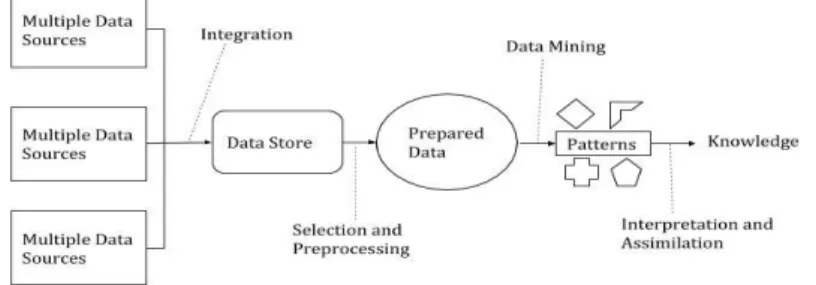
Into this vision, data mining is considered as a step concerned with the algorithmic part to find patterns from the data (Kaur, 2014). Frawley (1992) defines Knowledge Discovery as the nontrivial extraction of useful information from data that was not known before. KDD is based in five stages where it is always possible to come back to the previous step or other one that was made it previously. The processes are Selection, Pre-processing, Transformation, Data mining and Interpretation/Evaluation (Fayyad, et al., 1996b; Bramer, 2007; Han, et al., 2012).

Figure 1- Knowledge Discovery in Databases process (Adapted from (Bramer,

5

In Figure 1 is possible to verify the KDD process. There is a multiple quantity of data sources providing data that will be integrated in some common data store and a part will be taken and pre-processed to a standard format. Using this prepared data, it will be initialized the data mining process where it will be applied techniques and methods in the data which will produce an output in some type of pattern format. Patterns are the raw material to knowledge discovery that, when is applied interpretation on it, is possible to achieve potentially useful knowledge (Bramer, 2007; Han, et al., 2012).

The biggest targets of knowledge discovery vary depending on the use that will be given to the system, where it is possible to define between two goals. One of these goals are verification, where the system is based on user hypothesis tests. The other are discovery, where the system finds patterns by himself. In discovery it is possible to split it in two parts: prediction and description. Prediction finds patterns to predict the future behaviour of some entities and description is where the system finds patterns to provide to the user on an understandable format (Fayyad, et al., 1996a; Fayyad, et al., 1996b). Data-mining is involved with knowledge discovery goals because it provides the methods to achieve them.

2.2 Data mining methods

The most common methods are classification, regression, clustering and summarization (Kumbhare & Chobe, 2014; Han, et al., 2012). Clustering is a method used to discover groups in a set of objects where there are not a response variable (Han, et al., 2000). Summarization is a method that provide a compact representation of the data set which can include visualization and report generation (Kumbhare & Chobe, 2014).

Classification and regression has the same general mathematical and statistical underpinnings, but they are applied to different specifications. Classification is a process with the goal of finding a model that has the capacity to distinguish classes, where the response variable is the class that we want to achieve, mapping a vector of measurements from the independent variables/explanatory

6

variables (Hand, et al., 2001; Han, et al., 2012). Furthermore, the model derives from a set of training data (Han, et al., 2012) which will be explained far ahead in what consists and how is it doing.

Regression is a set of statistics processes that is used for numeric prediction where is stablished a relationship between a dependent variable and one or more independent variables which the predicted response variable can be a value or a binary response value (Han, et al., 2012; Yan & Su, 2009; James, et al., 2013). The creation of a regression model also uses the same methodology than in classification, where is created the model from a set of training data. When the goal is prediction there are two usual data mining algorithms: the multiple linear regression when the response variable is a value, and the logistic regression when the response variable is binary (Han, et al., 2012).

Figure 2 – Core fields for Data Mining techniques (Adapted from (Han, et al., 2012))

In Figure 2 is possible to verify that data mining is a domain that integrate many techniques from any other fields. Looking to the multi-disciplinary environment that data mining is involved, it is understandable why data mining has so many success, research and constantly improvement and development.

Data Mining Techniques Machine Learning Statistics Pattern Recognition Visualization Algorithms Database systems Data warehouse Applications High-performance computing Information retrieval

7

2.3 Data mining components

DM is constituted by several methods to produce results. Many authors, to provide an understandable way of explaining data mining algorithms, define three primary components. The first component is model representation, which consists on the language used to describe discoverable patterns. In this component is very important to synthetize very clearly the assumptions that are made in the algorithm construction. Furthermore, it is also important to have a representation not very limited to provide a better training time and an accurate model (Fayyad, et al., 1996b; Fayyad, et al., 1996a). On this stage the model is created based on a training set (Clifton, n.d.). Model-evaluation is the second component which it is based in quantitative statements. Fit functions can be a statement that represents how well a pattern is accurate when the model is tested in another set. Depending on the type of KDD that is defined, different measures to evaluate will be used (Fayyad, et al., 1996b; Clifton, n.d.). The last component is the Search Method, which can be a parameter search or a model search. After model representation and evaluation has been fixed, the problem changes to an optimization task. This task is based on finding the parameters and models that optimize the defined evaluation criteria. When it is a parameter search, the model representation has been fixed and it is made a loop for the parameters that optimize the model evaluation given observed data. If it is a model search, it occurs a parameter search to find the best parameters that describe the model (Fayyad, et al., 1996b).

A discipline that provides tools to help the formulation of data mining algorithms like the previous described schema is machine learning. Machine learning algorithms providing ways to make model-selection, where it is usual to involve numerical optimisation, based on an estimator of generalization performance (Cawley & Talbot, 2010). For this constraint, it is usually used some tools that provide ways to validate the models (Hand, et al., 2001). These tools are very useful to create from a dataset a training data, also called training set, and a test data, also called validation set, test set or holdout set.

Train-test split, also called validation-set, and cross-validation are two of the most popular ways to validate models. The reason for this test is to prevent or, at

8

least minimize overfitting. Overfitting is a phenomenon that happen when the model that has been trained, was fitted too close from the training dataset. This is considered a problem because the model that has been generated possibly has low accuracy and/or is ungeneralizable (Cawley & Talbot, 2010). From other side, there are the possibility of underfitting. Underfitting happens when a model does not fit the training data properly, which means that the model misses the trends, and for that reason, the model cannot be generalized to another data (Everitt & Skrondal, 2010). It is more common to happen overfitting than underfitting (Harrel Jr, 2017). Overfitting and underfitting is known in machine learning field as overtraining and undertraining.

In train-test split is, as the name says, a technique where the data is usually split in two parts: one part will be used as training data and another will be used as test data (James, et al., 2013). On this strategy, recurring to measures of fitness on the training set/data, is found the model. The performance of the predicted model is consequently evaluated using it to calculate the predictions for the validation set. After calculating the predict values for the observations in the validation set, it is used the metrics presented further, like MSE, to analyse the model quality to predict (James, et al., 2013).

Cross-validation uses the same idea of train-test split but with some differences during the train-test formulation. In cross-validation, data is divided in more subsets than in train-test split where the goal is testing the ability of a model to predict new data that was not used to generate it, with precaution to problems like overfitting (Hand, et al., 2001). To achieve the goal, cross-validation combines recurring to the average, measures of fitness in prediction to develop a more accurate estimate of model prediction performance (Seni & Elder, 2010).

From a large quantity of cross-validation methods, the two more famous are K-Folds Cross-Validation and Leave One Out Cross-Validation. In K-Folds method, the data is split into k different subsets, also called folds. To train the data, it is used

k-1 folds and the last fold is used as test data. Furthermore, after all the folds being

used, it is calculated their average with each of them. Subsequently to this procedure the model is tested against the test set (Seni & Elder, 2010). In Leave One Out

9

method is repeated the idea of K-Folds, but on this case the number of folds will be the number of observations present in the dataset. The next step will be average all the folds and construct the model with it. After this procedure, the model will be tested against the last fold that was not used for train (Hand, et al., 2001). Scikit, a machine learning library for Python, reveals to be a very useful tool for this treatment, having an object that provides an easier way to do test-train split and a wide variety of cross-validation algorithms (Pedregosa, et al., 2011).

There are several quantities of tools to work with data mining algorithms in Python. Two of the most popular options are Statsmodels and Scikit-learn. Statsmodels is a Python package that as part of the scientific Python stack oriented towards data analysis, data science and statistics. Statsmodels is a complement of SciPy, that has efficient algorithms for linear algebra, sparse matrix representation, special functions and basic statistical functions (Pedregosa, et al., 2011). Statsmodels has a close syntax to R language which can be an advantage for people that are transitioning to Python (Sutton, 2018). The results of their algorithms are verified with, at least one other statistical package (Statsmodels, n.d.). Scikit-learn is a Python module, integrating a wide rich group of machine learning algorithms, an easy-to-use task-oriented interface closely integrated with the Python language, and it reveals a good answer for the growing development of statistical data analysis (Pedregosa, et al., 2011). Both can co-work together because they share the same base data structure for data and model parameters, providing for a tool called NumPy (Pedregosa, et al., 2011). An analysis reveals that users Statsmodels are usually related to statistics and econometric tools and users of Scikit are related with data analysis (Sutton, 2018).

2.4 Data mining algorithms

There are several number of data mining algorithms. Some examples of them are Multiple Linear Regression, Logistic Regression, Linear Correlation Coefficient and Association Rule Mining.

10

2.4.1 Multiple Linear Regression

Multiple linear regression is a type of regression model that is used to design a linear approach to modelling a dependent variable and one or more independent variables. Linear regression is a method used to find the best response line to fit two variables, so that one of them can be used to predict the other. Multiple linear regression as the same idea, but there are more than two variables involved (Han, et al., 2012; Chatterjee & Hadi, 2012; Newbold, et al., 2013).

Y = aX + b + error

Where a and b minimize the error of the Y predicted, given range of values of X. Multiple linear regression is composed with Y , that represents the dependent variable values matrix, a, represents the beta group matrix, b, the intercept matrix, also called constant, and the observed errors matrix (Yan & Su, 2009; Chatterjee & Hadi, 2012; Newbold, et al., 2013).

Regression has some assumptions to be used. The assumptions are the presence of linear relationship between variables, the variables should have a normal distribution or a very close proximity with a normal distribution. Another assumptions to take care about are, the data does not have multicollinearity or there are just a little, that means that the independent variables should not be very highly related to each other, the data should not have autocorrelation which means that the residuals should be independent from each other and the data should be homoscedastic, it means that the residuals are equal across the regression (Newbold, et al., 2013).

To test the predicted models there are a group of metrics that provide the possibility to analyse it. Machine learning development brings more possibilities of techniques to make tests and improve their robustness and, on this way, improving the quality of the models and, giving more ways to evaluate it. There are multiple techniques for multiple linear regression evaluation, like the mean absolute error (MAE), the mean squared error (MSE) and the coefficient of determination (R2_).

MSE is a measure of precision that represents the mean of the squares of the errors for N pairs of values. Errors is the difference between the observed (o) and the

11

predicted values (p) (o and p will represent the same in all the formulas) (James, et al., 2013; Scikit-learn, n.d.; Lehmann & Casella, 1998).

𝑀𝑆𝐸 = 1

𝑁∑(𝑜𝑖 − 𝑝𝑖 )

2 𝑁

𝑖=1

MAE represents the mean magnitude of the absolute value of the errors. In MAE is not considered the direction of the errors and, all of them, have equal weight (Willmott & Matsuura, 2005).

𝑀𝐴𝐸 = 1

𝑁∑|𝑜𝑖 − 𝑝𝑖|

𝑁 𝑖=1

Exploring Scikit metrics for model evaluation, it was found a metric that was not talked on the explored literature, called Median Absolute Error (MedAE). Median absolute error is an interesting measure because it is robust to outliers. MedAE is calculated with the median of all the absolute differences between the target and the prediction (Scikit-learn, n.d.).

𝑀𝑒𝑑𝐴𝐸(𝑜, 𝑝) = 𝑚𝑒𝑑𝑖𝑎𝑛(|𝑜₁− 𝑝₁|, … , |𝑜𝑖 − 𝑝𝑖| )

One other measure to evaluate the prediction is the coefficient of determination, also called R squared. The coefficient of determination is a measure that evaluate how well future samples are likely to be predicted by the model (Nagelkerke, 1991). Usually, the coefficient of determination is a value between 0 ≤ R2 _{≤ 1 (Draper & Smith, 1998). There are many ways to calculate the R squared and}

can be given by the following ratio (Newbold, et al., 2013):

𝑅2(𝑜, 𝑝) = 1 −𝑆𝑆𝑟𝑒𝑠 𝑆𝑆_𝑡𝑜𝑡 = 1 − ∑𝑛𝑠𝑎𝑚𝑝𝑙𝑒𝑠−1(𝑜_𝑖 − 𝑝_𝑖)2 𝑖=0 ∑ (𝑜𝑖 − 𝑜̅𝑖)2 𝑛𝑠𝑎𝑚𝑝𝑙𝑒𝑠−1 𝑖=0 where 𝑜̅ = 1 𝑛𝑠𝑎𝑚𝑝𝑙𝑒𝑠∑ 𝑜𝑖 𝑛𝑠𝑎𝑚𝑝𝑙𝑒𝑠−1

𝑖=0 , 𝑆𝑆𝑟𝑒𝑠 represents the sum of squares error and

𝑆𝑆_𝑡𝑜𝑡 is the sum of squares regression (Newbold, et al., 2013).

When applied to prediction in testing data for estimation in machine learning, it is possible to see negative values on R2_{. This happens because there is a difference}

12

between the definition of R squared and his estimation. There are several formulas for estimation the R squared and, in some of them it is possible to have, without unrespect mathematical rules, a negative value. Like in Nash-Sutcliffe model efficiency coefficient (NSE) which is used to assess the predictive power of hydrological models and, when the total sum of squares can be partitioned into error and regression components, which is equivalent to the coefficient of determination, the value can be negative. In NSE the coefficient values can range from ]−∞; 1] (Moriasi, et al., 2007).

When the efficiency has value of 1, this means that the model is more accurate than the mean of the observed data. Values between 0 and 1 are considered as acceptable performance levels. If there are an efficiency of 0, this indicates that the model is as accurate as the mean of the observed data. When the value is negative, it means that the model is worse to predict than the mean of the observed data, which is a signal of a bad performance (Moriasi, et al., 2007). The reason for the possibility to have a negative value lays on the fact of the predicted model does not follow the trend of the data which means that the model fits worse than the mean of the observed data or because of the inexistence of an intercept (Scikit-learn, n.d.).

2.4.2 Logistic regression

Logistic regression is a type of model that address the relationship between a binary dependent variable Y (can be true or false, zero or one, etc.) and one or more independent variables Xm, where m represents the number of independent

variables, combined with a 𝛽I, coefficient parameter, and a constant 𝛽₀ (Faul, et al.,

2009; Hand, et al., 2001).

𝑙𝑜𝑔𝑖𝑡(𝑌) = 𝛽₀+ 𝛽₁. 𝑋₁+ 𝛽₂. 𝑋₂+ ⋯ + 𝛽_𝑚. 𝑋_𝑚

In logistic regression, the prediction model is normally recognized by the accuracy. For this procedure, it is generally analysed the accuracy score and, it is also used a confusion matrix where is possible to see how many times the model predicts correctly. The confusion matrix is composed by four possibilities: the model predicts one and it is, the model predicts one, but the sample is zero (the model

13

fails), the model predicts zero and it is, and the model predicts zero and the sample is one (the model fails) (Fawcett, 2006; Bramer, 2007; Han, et al., 2012). The accuracy of a model is basically, the number of times that the model evaluates correctly. There are many times a misunderstanding about accuracy because the dataset can be unbalanced, which means that there are not the same number of observations for the two classes and, for this reason, the accuracy is not completely reliable (Han, et al., 2012; Bramer, 2007).

2.4.3 Pearson Correlation Coefficient

Pearson correlation is a measure way to calculate the linear correlation between two variables, X and Y, where both are standardized and normalized. The coefficient values vary between [-1, 1], where 1 represents a positive linear correlation, 0 means no linear correlation, and -1 is negative linear correlation. The coefficient does not mean que quantity of proportionality but if they are linearly related. For a statistic sample r, the formula for calculating the coefficient is given by (Swinscow & Campbell, 1997):

𝑟 = ∑ (𝑥𝑖− 𝑥̅)(𝑦𝑖− 𝑦̅)

𝑛 𝑖=1

√[∑𝑛𝑖=1(𝑥𝑖 − 𝑥̅)2][∑𝑛𝑖=1(𝑦𝑖− 𝑦̅)2]

Where 𝑥_𝑖 and 𝑦_𝑖 are the values of x and y for the ith _{individual observation.}

2.4.4 Association Rule Mining

Another topic related to DM is association rule mining (ARM). ARM has been one of the subjects with major interest for researchers. An association rule is an association technique that has an expression N → O, where N and O are sets of items, that means, given a database R of transactions T, where each transaction T ∈ R is a set of items, N → O represents that whenever a transaction T contains N, then T probably contains O also. This probability or rule confidence can be understood as the conditional probability p(O|N) = p (O ⋂ N) / p(N) and it is represented as the percentage of transactions containing O in addition to N, regarding the overall number of transactions containing N (Hipp, et al., 2000; Han, et al., 2000; Kumbhare

14 & Chobe, 2014; Kaur, 2014).

ARM is a method used to find frequent patterns, correlations, associations or causal structures from data sets found in many types of data repositories such as relational databases and transactional databases, etc. (Kumbhare & Chobe, 2014; Kaur, 2014; Tan, et al., 2006; Hand, et al., 2001; Han, et al., 2012).

This is a very useful method to give help for business decisions in organizations, like retailers with a large collection of items or in another fields and areas such as medical diagnosis, inventory control, telecommunication networks, risk and market management etc. The spinal use of ARM has been in market basket data analysis, to analyse the association of purchased items in a single basket/purchase, in cross-marketing to work with other businesses that complement the organization business, providing an idea for which partnership could be interesting to do to increase the organization revenues, status, etc, and in catalogue design, to find which items are very related, in order to create a better business catalogue designed to complement each other (Kaur, 2014). Looking to these applications we can say that ARM is useful to the organizations allowing them to find a way of cross-selling and up-selling their products. Their proprieties can be also useful for another subject where the target is finding associations.

Many research has been done and a lot of algorithms have been appeared, but it still exists many issues and development to do in this field. The main drawbacks of the ARM algorithms are essentially, the fact that the algorithms obtain non-interesting rules, a huge number of them can be discovered and, it still existing a low algorithm performance (Kaur, 2014). The only factor that contributes to the beginning of the algorithm is minimum support (minsup). The minsup is the minimum support than an item must have to be considered frequent and. The minsup is commonly a user configuration. Only exists a single minsup, which means that all the items are of the same nature, which cannot be always the case. One example is in retailing business, when can happen a different behaviour for price reasons. In retail the customers frequently tend to buy the items that has less price, and the relationships between these items cannot be similar for the same product that has a higher price. If the minsup is set too high these items will be frequently

15

the patterns and this is not helpful for the organizations because this associations brings small profits comparably with the same products that has higher price. This problem is called as rare item problem (Kaur, 2014; Tan, et al., 2006). Another problem that happen is the privacy, where must happen a treatment to hide the sensitive information (Kaur, 2014).

2.4.4.1 Formal problem of Association Rule Mining

Let χ = {c1, c2, …, cm} be a set of items. A set C ⊆ χ with k =|C| is called a k-itemset

or an itemset. Let B represent relevant data transactions sub-sets of χ. Each T ∈ B represents a transaction which contains a transaction identifier (TID). Each transaction has a different TID. A transaction T ∈ B supports an itemset C ⊆ χ if C ⊆ χ holds. An association rule is constituted with an antecedent and a consequent part with an expression C → A, where C and A are itemsets and C ⋂ A = ∅ holds (Hipp, et al., 2000; Kaur, 2014; Kumbhare & Chobe, 2014; Tan, et al., 2006). An antecedent is an item found in data and, a consequent is an item that it was found combined with the antecedent. The ARM works based on a support-confidence framework. To get the association rules, firstly it is necessary to calculate the support (supp). Support is defined than the portion of transactions T, where exists the itemset C inside the database B. The expression is:

𝑠𝑢𝑝𝑝(𝐶) = |{𝑇 ∈ 𝐵| 𝐶 ⊆ 𝑇 }|/|𝐵|

The support of a rule C → A is defined as supp (C → A) = supp ( C ∪ A) . After the support has been found it is possible to calculate the confidence (conf). The confidence of a rule is defined as:

𝑐𝑜𝑛𝑓(𝐶 → 𝐴) =𝑠𝑢𝑝𝑝 ( 𝐶 ∪ 𝐴) 𝑠𝑢𝑝𝑝(𝐶)

On this function C is the antecedent and A represent the consequent part. That means that it is calculated the groups where exists C and A inside the itemsets of C. In this method is usually used a minimum support (minsup) and a minimum confidence (minconf) value. The minconf is the minimum confidence that an association rule must have to be considered relevant and it is usually a user configuration. The reason of that is the fact of this type of method is recurrently used

16

in big datasets that grows exponentially with | χ |, which means the possibility of existence of a huge number of rules and, as consequence, a huge computational expense cost. With these two restrictions is possible to reduce the number of rules to be generated and, split the task in two parts (Han, et al., 2012; Tan, et al., 2006; Han, et al., 2000; Kaur, 2014; Kumbhare & Chobe, 2014):

a) Frequent itemset generation, where the target is find all the itemsets that have a transaction support above the minimum support. The itemsets that respect the minimum support are called large itemsets. The itemsets that has a lower value than minsup are pruned and it will be not used in the following steps.

b) Rule generation, where it is used the large itemsets to generate the rules. Inside every itemset g is necessary to find all the subsets to create all the possible consequents and antecedents. For every such subset s, is created a rule of form s → (g − s). In this step it is calculated the confidence of the rule and if it has at least the minconf value it will be outputted.

In association patterns there are multiple metrics that can be used to disseminate information. One of the reasons for that is the limitations of the support-confidence framework, where there is the possibility to find a huge group of patterns but not all of them can have good quality. Furthermore, the confidence values can overrate the rules. This can happen because the same rule can be higher for the both sides, each means that it can happen the existence of rules that are profitable working in the opposite way (Tan, et al., 2006; Han, et al., 2012; Kumbhare & Chobe, 2014). Another popular measure, which it is a way to avoid the misleading of the confidence measure, is the lift metric, which gives the ratio between the confidence of a rule and the support of his consequent (Tan, et al., 2006; Kumbhare & Chobe, 2014). Beyond this metrics the are several more to apply in ARM (Tan, et al., 2006).

𝐿𝑖𝑓𝑡 = 𝑐𝑜𝑛𝑓 (𝐶 → 𝐴 ) 𝑠𝑢𝑝𝑝(𝐴)

17

2.4.4.2 Association Rule Mining common algorithms

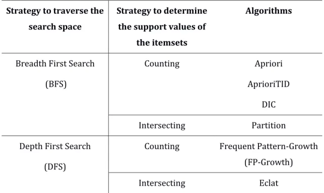
As an attractive subject for many researchers, the development in ARM has been happening providing many algorithms to do that task with different perspectives and constructions and their way to work have some differences. Although their differences they share the same basic idea that it was said before. The algorithms can be characterized by two types of strategy (Table 1) (Hipp, et al., 2000):

a) by its strategy to traverse the search space and;

b) by its strategy to determine the support values of the itemsets.

Table 1 - Systematization of the most common algorithms of ARM (adapted from (Hipp, et al., 2000))

Strategy to traverse the search space

Strategy to determine the support values of

the itemsets

Algorithms

Breadth First Search (BFS)

Counting Apriori

AprioriTID DIC

Intersecting Partition

Depth First Search (DFS)

Counting Frequent Pattern-Growth (FP-Growth)

Intersecting Eclat

BFS is an algorithm for traversing or searching tree or graph data structures. This algorithm starts at the tree root or some arbitrary node, and explores firstly all the neighbour nodes at the present depth level before moving to the nodes at the next depth level (Cormen, et al., 2001; Hipp, et al., 2000). The most popular algorithm inside this methodology is Apriori. Apriori appeals to a test group candidate against the data. The algorithm uses k-itemsets (with size k) to explore

18

(k+1)-itemsets and find frequent itemsets/patterns from the database for Boolean association rules (Kumbhare & Chobe, 2014; Hipp, et al., 2000; Hand, et al., 2001; Han, et al., 2012). Into the frequent itemset generation, Apriori uses frequent subsets to find candidates in the data, counting the support of the itemsets and, this ones that respect at least the minsup, are used to extend, this it means that Apriori find frequent itemsets by doing multiple scans (Tan, et al., 2006; Kumbhare & Chobe, 2014; Kaur, 2014).

Apriori has a property for pruning, that means that only the subsets that respect the minimum support for each extension are used to the next candidate generation extension step (Hipp, et al., 2000; Tan, et al., 2006; Han, et al., 2012; Hand, et al., 2001; Kumbhare & Chobe, 2014). Afterwards, the algorithm generates all the possible combinations of candidates that is possible to create with the subsets that respects the minsup. The maximum size that a frequent itemset can have is equal to the maximum length of the biggest itemset into the database. The candidate generation step stops when there is not exist candidate subsets that respect the minimum support or, when it comes to the maximum size of itemsets existent on the database.

The advantages of Apriori are the fact of this algorithm has an easier implementation comparably against other possible algorithms of ARM and, it uses Apriori property for pruning, which is a useful property (Kaur, 2014). The biggest drawbacks of Apriori lives on the fact of this type of algorithm requires multiple scans into the database, with a complex candidate generation process, which consumes a lot of time, space and memory (Kaur, 2014; Tan, et al., 2006).

In DFS the way that the algorithm works is exactly the opposite. Firstly, the algorithm will explore the highest depth nodes, and it will be forced to backtrack and expand another node (Cormen, et al., 2001; Kumbhare & Chobe, 2014; Hipp, et al., 2000). The most popular algorithm that use this strategy is Growth. FP-Growth can be considered as an improvement of Apriori algorithm.

The generate-and-test paradigm of Apriori is not used in Growth. FP-growth works without candidate generation (Han, et al., 2000; Han, et al., 2012; Agrawal & Srikant, 1994). On this one, it is used an FP-tree with all the frequent

19

items and it is extracted from their structure all the frequent itemsets (Hipp, et al., 2000). FP-growth only needs two scans into the database to gather all the information that it needs.

The first scan of the algorithm is used to compute a list containing all the frequent items (Tan, et al., 2006; Kumbhare & Chobe, 2014). These frequent items will be sorted in descending order taking account their absolute support, it means, the number of times than an item occurs into the database. On the second scan, it is compressed the database taking the form of a tree. The process for the tree creation stops after every transaction has been mapped to a path (Tan, et al., 2006; Han, et al., 2000; Kumbhare & Chobe, 2014). This algorithm performs mining on FP-tree recursively (Kumbhare & Chobe, 2014; Han, et al., 2000). Many different transactions can have several items in common and, for that reason, it will be generated a more compressed FP-tree structure because their paths will overlap (Tan, et al., 2006).

The size of an FP-Tree varies depending on the compressibility of the data, how much more items are in common between transactions and more compressed will be the tree. Another factor that make the size of an FP-tree vary is how the items are ordered by support. Commonly the items are ordered in descending order of support. Many times, this fact leads to the smallest tree but not always (Tan, et al., 2006; Kumbhare & Chobe, 2014).

FP-growth also uses a conditional FP-tree, which is like an FP-tree in terms of structure. On this case, the conditional FP-tree is used to find frequent itemsets ending with a suffix. Into this suffix is solved all the subproblems that involves the suffix itself and while suffix is joined with others. This approach is the biggest key of FP-growth which it is known as divide-and-conquer approach (Han, et al., 2000; Tan, et al., 2006; Kaur, 2014; Kumbhare & Chobe, 2014). Several studies, were made to compare some algorithms against each other, conclude that the algorithm that has the best performance is FP-growth, based on a performance perspective (Kumbhare & Chobe, 2014).

20

3.

M

ETHODOLOGY

On this work it was followed a Design Science methodology. Design-Science is a problem-solving paradigm in Information Systems that follows the design of useful artifacts that extend the boundaries of human problem solving and organizational capabilities by providing intellectual and computational tools, where the artifacts are defined as constructs, models, methods and instantiations (Hevner, et al., 2004).

Artifacts are innovations that define the ideas, practices, technical capabilities, and products through which the analysis, design, implementation, and use of information systems can be effectively and efficiently accomplished (Hevner, et al., 2004) Artifacts can take, from so many, the format of algorithms, human/computer interfaces, and system design methodologies or languages (Vaishnavi, et al., 2017), which must be evaluated in order to ensure is utility for the specified problem. It was developed several guidelines to describe the requirements for a design-science research (Hevner, et al., 2004).

Design as an Artifact is one of these guidelines, which is applied on this work. The artifact produced is the system for association patterns, for a Linux Ubuntu software, that provides a report that facilitates the understanding of the output results. The system performs important statistical elements, analyse and evaluate the created models using a group of metrics which will be interpreted to guide the user. The system also provides an algorithm for association rule mining.

Another guideline that can be applied on this work is problem relevance. The problem that was treated is one of the most important topics to the organization in the moment. The system target is evading statistical misunderstandings, simplify the data analysis task for people with low knowledge, provide a tool that can help small business to find associations in their data and formulate interesting models to lead with business and management problems, creating insights about the topic in study to the user.

A third guideline that applies to this problem is design evaluation. The system was evaluated by the output accuracy of the results. It was used an analytical design evaluation methodology. To make the evaluation, the system results was compared against another analytic tool for regression (Excel) (Appendix 1). For FP-growth

21

algorithm it was used an experimental evaluation methodology, using artificial data to verify the results.

Research contribution is another guideline that is applied to this project. Providing guidance interpretation for statistical results is possible to avoid bad model formulations. General outputs from analytic tools only generate numerical results which can cause many misunderstandings for people with low knowledge in statistics.

Research rigor guideline also is applied. All the models that has been developed are result from many years of research and strong dissemination. All these models are core instruments of data analysis.

22

4.

R

ESULTS

The aim of this system is to serve as a small support system to the users. By delivering models and reports, the system helps the users in the decision-making process.

Associate things are one of the most typical line thinking of people, that means into the data analysis process this also happen. Taking by definition of association the fact of being involved with or connected to someone or something (Cambridge University Press, n.d.), the state of being associated: combination, relationship (Merriam-Webster, n.d.), and for association patterns, descriptions of the semantics that define common types of associations, or structural relationships, that occur between objects (Ehlmann, 2009), is possible to say that Multiple Linear Regression (MLR), Logistic Regression (LR), Linear Correlation (PC) and Association Rule Mining are examples of data mining algorithms that provide associative patterns.

Multiple Linear Regression and Logistic Regression belonging to this definition because they relate a dependent variable response with one or many independent variables, Correlation makes the same, testing the possibility of relation between two variables. Association Rule Mining because it is tested the existence of associations between objects.

For each type of association pattern that was referred before, it was created a model to work with each of them. In multiple linear regression, logistic regression and Pearson correlation it was implemented Statsmodels and Scikit packages to work with the data. For ARM it was created a FP-growth algorithm. The decision for FP-growth against other possible models for association rule mining was taken by the unusual methodology and because, as described previously, FP-growth was considered the algorithm with the best performance (Kumbhare & Chobe, 2014). In FP-growth it was assumed that each line of the table as an item and there is a transaction identifier, where it will be joined all the items that belongs to the same identifier.

23

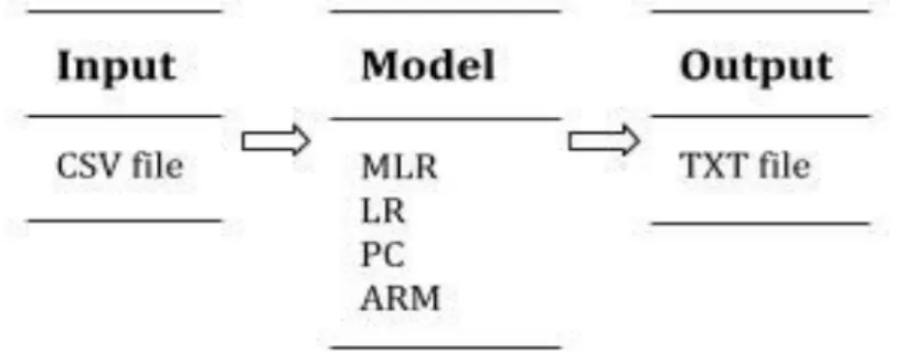
Figure 3 - System workflow

The system has a simple workflow (Figure 3). It receives as input CSV files, where the first line represents the names of each label. It is assumed that the data was already pre-processed, normalized and standardized, without missing values and data is in good conditions to be used.

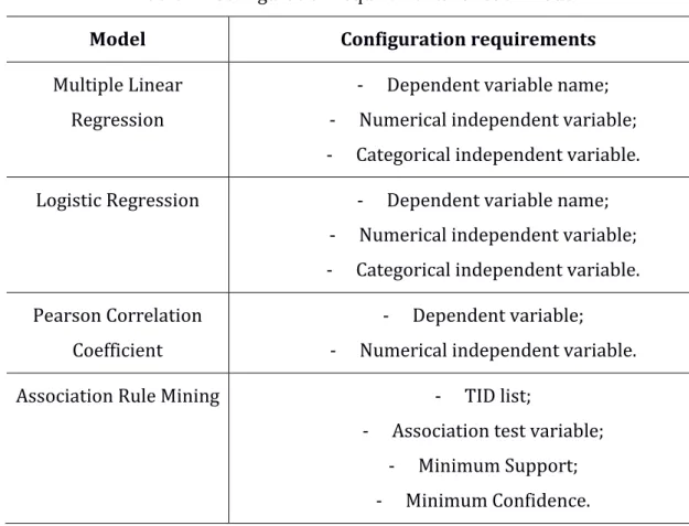
The user has a configuration page where he chooses the model that he wants to use for modelling the data. The user chooses the columns that he wants to use in the model also reveals their format (Table 2)(Appendix 2). It means that it is necessary to define the name of the variable in the configuration requirement that it belongs. Each model has variables and different configuration requirements. Some variables need to be configurate to have a valid format to be used. The categorical variables, that represent a variable with categories, are one of these variables. It is created a dummy variable to represent the categories. The dummy variable will have a binary character that represent the presence or absence of a category for each line. If there are k categories, it is necessary k-1 tables to take all the information needed. In association rule mining there are also a change in the data. The variable that represents the association test variable will change if there are more than one line with the same TID. In that case it is joined all the items of the association test variable, which means that it is created an array with all the items that exist in the same TID.

Consequently, it is generated a report with the output results and the interpreted requirements in TXT format. Each output will be different depending on the type of the model that it is used.

24

Table 2 - Configuration requirements for each model

Model Configuration requirements

Multiple Linear Regression

- Dependent variable name; - Numerical independent variable; - Categorical independent variable. Logistic Regression - Dependent variable name;

- Numerical independent variable; - Categorical independent variable. Pearson Correlation

Coefficient

- Dependent variable; - Numerical independent variable.

Association Rule Mining - TID list;

- Association test variable; - Minimum Support; - Minimum Confidence.

In regression models (multiple linear regression and logistic regression) it was used Scikit-learn train-test split approach to split the data into a part of train and test. It was defined 75% of the sample as training data and all the rest will be used to test the predicted model.

The biggest part of the data will be used as training to create a robust model that has the capacity to catch the trends of the data. To generate the model with the training data it was used Statsmodels regression package. The method of multiple linear regression used was the ordinary least squares. The reason for this decision was the fact of Statsmodels output has a close format to the R package.

All the prediction evaluation metrics that has been created came from Scikit (Appendix 3; Appendix 4; Appendix 5; Appendix 6). For Pearson correlation it was used a tool from SciPy (Appendix 7). For FP-growth algorithm it was developed all the code, using also some Python libraries (Appendix 8; Appendix 9).

25

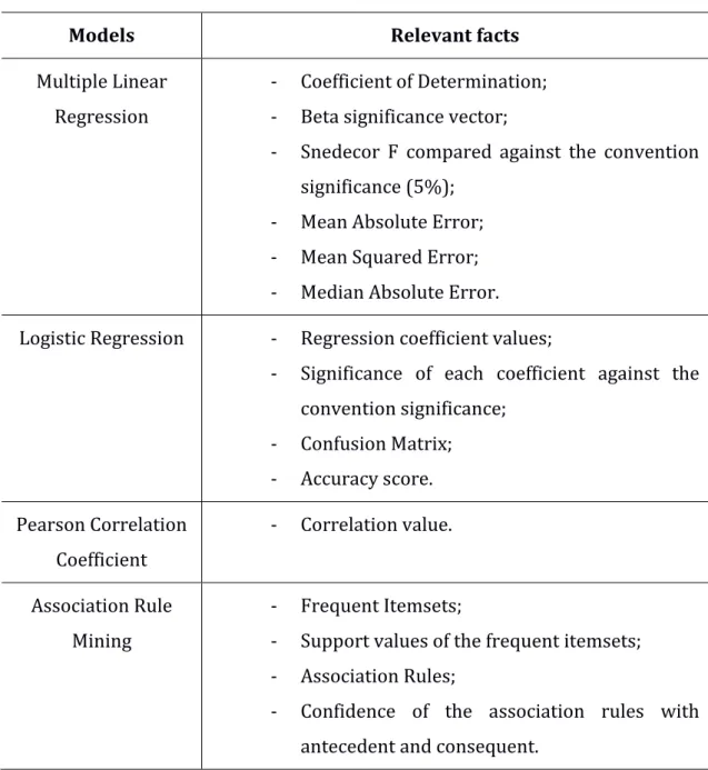
results and looking to what it is the most important values to be analysed when it is created a model, providing interpretation and results for all the models. In Table 3 is showed what is considered a relevant fact for each model created in the system.

In regression is possible to split the guidance in two parts. Firstly, it is given a guidance about the most important statistical aspects of the predicted model. On this part, in multiple linear regression, it was given special attention to the Snedecor F significance, comparing to the convention significance, and for the beta significance of each variable, also comparing to the convention significance. In logistic regression it was given special attention to the beta significance of each variable. The second part consists on the results of the predicted model in the test data. It is given measures and guidelines about the results (Appendix 11; Appendix 12; Appendix 13; Appendix 14). In multiple linear regression it is given the mean squared error, the mean absolute error and the median absolute error. To the logistic regression it is provided a confusion matrix and the accuracy score of the model.

For the linear correlation coefficient, where is used the Pearson Correlation Coefficient method, it is given the results of the comparison between the two variables (Appendix 15).

In association rule mining it is provided the frequent itemsets of the data, their support, the association rules where it is identified the consequent and antecedent. The antecedent was constructed to work only with an item. To evaluate the association rules, it is provided the confidence values (Appendix 16; Appendix 17). It is only displayed the values itemsets and the association rules that respect the minsup and minconf values, respectively. All the possibilities of association rules with different antecedents and consequents that respect the minconf are displayed.

26

Table 3 - Relevant results to be analysed for each model

Models Relevant facts

Multiple Linear Regression

- Coefficient of Determination; - Beta significance vector;

- Snedecor F compared against the convention significance (5%);

- Mean Absolute Error; - Mean Squared Error; - Median Absolute Error. Logistic Regression - Regression coefficient values;

- Significance of each coefficient against the convention significance; - Confusion Matrix; - Accuracy score. Pearson Correlation Coefficient - Correlation value. Association Rule Mining - Frequent Itemsets;

- Support values of the frequent itemsets; - Association Rules;

- Confidence of the association rules with antecedent and consequent.

27

5.

C

ONCLUSIONS

On this work it was possible to deeply understand the data mining techniques that was been created in the system, improve the knowledge about Python applied to data analysis, understand the conceptualization of the data mining techniques, both logically and applicational. It was comprehended how machine learning algorithms are applied in Python and the benefits of use a programming language with so many resources instead of an analytical tool. With this project it was possible to understand what association rule mining is, the concepts that are included, the algorithms implemented for this task and the complexity that is involved in algorithms of this kind.

With the benefits that was viewed, it becomes clear why the market growth of Python and why Python is a big threat for many analytical tools. Its flexibility, robustness, clear syntax and facility to generate tools for data analysis, with the huge number of libraries. These facilities help data analysts to work with data on their way and gives the opportunity of structure analysis more complex and robust to them.

It was possible to create the proposed system for these data mining techniques, that was the biggest goal to this thesis, which can help many users with low knowledge in statistics. The system also reveals values close to another analytic tool which prove that is possible to formulate good models with machine learning algorithms. Although all the success of the construction, many methods could be created on different way, using more robust components, like a cross-validation technique in the regression models. Being a more robust technique, it will produce more accurate results. In FP-growth also could be joined a wider group of metrics. Any other methods also could be implemented, but it requires much more time to develop. One design evaluation methodology that could be applied, was the validation of the report from management people, where the quality of report could be evaluated to verify if the system increases the understanding on the implemented models.

28

type, even worse when exists a small background. This activity involves several knowledges about a programming language, understand their syntax, how it works, which existent machine learning are and what they support.

It is also concluded that, the use of programming languages to work with data should be encouraged because, even if it is created a system from a programming language, the data analysts are limited to a group of options which can be not enough for many studies.

In data mining there are severe amounts of tools, research and constant development. It was possible to verify that data mining is an unquestionable topic in development nowadays, with many recent literatures being produced. One of the most important parts that also contributes for data mining developed is the concise definition of each method. Nowadays, data analysis can be done simpler with the huge amount of machine learning algorithms that already exists helps on this task and can be easily incremented their complexity.

With contribution for future works, after being passed for all the construction stages of development of some data mining techniques, it was thought, to provide some statistical knowledge for students of management information system, that can be an interesting idea the development of a group test where statistics is teach based on Python machine-learning, where it is compared the performance of students using the traditional approach against students that learn using this type of methodology. Other projects of this kind can be made it improve the knowledge about another data mining techniques, where visualization could be applied because with visualization is possible to have a better idea of the data.

29

R

EFERENCES

Agrawal, R. & Srikant, R., 1994. Fast Algorithms for Mining Association Rules. Santiago, Chile, s.n.

Apte, C., Liu, B., Pednault, E. P. & Smyth, P., 2002. Business Aplications of Data Mining. Communications of the ACM, Volume 45, pp. 49-53.

Bramer, M., 2007. Principles of Data Mining. s.l.:Springer.

Cambridge University Press, n.d. Cambridge Dictionary. [Online] Available at: https://dictionary.cambridge.org/dictionary/english/association [Accessed 25 April 2018].

Cawley, G. C. & Talbot, N. L. C., 2010. On Over-fitting in Model Selection and Subsequent Selection Bias in Performance Evaluation. Journal of Machine Learning

Research 11, pp. 2079-2107.

Chatterjee, S. & Hadi, A. S., 2012. Regression Analysis By Example. Fifth ed. s.l.:Wiley.

Clifton, C., n.d. Encyclopædia Britannica. [Online] Available at: https://www.britannica.com/technology/data-mining [Accessed 29 Setembro 2018].

Cormen, T. H., Leiserson, C. E., Rivest, R. L. & Stein, C., 2001. Introduction to Algorithms. In: s.l.:MIT Press and McGrath-Hill, pp. 531-549.

Draper, N. R. & Smith, H., 1998. Applied Regression Analysis. s.l.:Wiley-Interscience.

Ehlmann, B. K., 2009. Association patterns for data modeling and definition, s.l.: Springer.

Everitt, B. S. & Skrondal, A., 2010. The Cambridge Dictionary of Statistics. s.l.:Cambridge University Press.

Faul, F., Erdfelder, E., Buchner, A. & Lang, A.-G., 2009. Statistical power analyses using G*Power 3.1: Tests for correlation and regression analyses. Behavior Research

30

Fawcett, T., 2006. An introduction to ROC analysis. Elsevier, Volume 27, pp. 861-874.

Fayyad, U., Piatetsky-Shapiro, G. & Smyth, P., 1996a. Knowledge Discovery and

Data Mining: Towards a Unifying Framework. s.l., AAAI.

Fayyad, U., Piatetsky-Shapiro & Smyth, P., 1996b. From Data Mining to Knowledge Discovery in Databases. AI Magazine, Volume 17, pp. 37-54.

Hand, D., Mannila, H. & Smyth, P., 2001. Principles of Data Mining. s.l.:The MIT Press.

Han, J., Kamber, M. & Pei, J., 2012. Data Mining: Concepts and Techniques. Third ed. s.l.:Elsevier.

Han, J., Pei, J. & Yin, Y., 2000. Mining Frequent Patterns without Candidate Generation. ACM SIGMOD Record.

Harrel Jr, F. E., 2017. Regression Modeling Strategies. s.l.:Spring.

Hevner, A. R., Ram, S., T.March, S. & Park, J., 2004. Design Science in Information Systems Research. MIS Quaterly, March, pp. 75-105.

Hipp, J., Guentzer, U. & Nakhaeizadeh, G., 2000. Association Rule Mining - A General Survey and Comparison. SIGKDD Explorations.

James, G., Witten, D., Hastie, T. & Tibshirani, R., 2013. An Introduction to

Statistical Learning with Applications in R. s.l.:Springer.

Kaur, G., 2014. Association Rule Mining: A Survey. International Journal of

Computer Science and Information Technologies, pp. 2320-2324.

Kumbhare, T. A. & Chobe, S. V., 2014. An Overview of Association Rule Mining Algorithms. International Journal of Computer Science and Information Technologies, Volume 5, pp. 927-930.

Lehmann, E. L. & Casella, G., 1998. Theory of Point Estimation. Second ed. s.l.:Springer.

Merriam-Webster, n.d. Merriam-Webster. [Online]

31 [Accessed 2 May 2018].

Moriasi, D. N. et al., 2007. Model Evaluation Guidelines for Systematic Quantification of Accuracy in Watershed Simulations. Soil & Water Division of ASABE, March.

Nagelkerke, N. J. D., 1991. A Note on a General Definition of the Coefficient of Determination. Biometrika, September, pp. 691-692.

Newbold, P., Carlson, W. L. & Thorne, B. M., 2013. Statistics for Business and

Economics. s.l.:Pearson Education, Inc..

Ollphant, T. E., 2007. Python: Batteries Included. Computing in Science &

Engineering, May/June, Volume 9, pp. 10-20.

Pedregosa, F. et al., 2011. Scikit-learn: Machine Learning in Python. Journal of

Machine Learning Research 12, pp. 2825-2830.

Scikit-learn, n.d. Scikit-learn. [Online]

Available at: http://scikit-learn.org/stable/modules/model_evaluation.html [Accessed 28 August 2018].

Seni, G. & Elder, J., 2010. Ensemble Methods in Data Mining: Improving Accuracy

Through Combining Predictions. s.l.:Morgan & Claypool Publishers.

Statsmodels, n.d. Statsmodels: Statistics in Python. [Online] Available at: https://www.statsmodels.org/dev/about.html [Accessed 10 June 2018].

Sutton, B., 2018. [Online]

Available at: https://blog.thedataincubator.com/2017/11/scikit-learn-vs-statsmodels/

Swinscow, T. D. V. & Campbell, M. J., 1997. Statistics at Square One. s.l.:BMJ Publishing Group.

Tan, P.-N., Steinbach, M. & Kumar, V., 2006. Introduction to Data Mining. First ed. s.l.:Pearson Addison-Wesley.

32 [Online]

Available at: http://desrist.org/design-research-in-information-systems/ [Accessed 15 September 2018].

Willmott, C. J. & Matsuura, K., 2005. Advantages of the mean absolute error (MAE) over the root mean square error (RMSE) in assessing average model performance. Climate Research 30, pp. 79-82.

Yan, X. & Su, X. G., 2009. Linear Regression Analysis: Theory and Computing. s.l.:World Scientific.

33

A

PPENDICES

Appendix 2 – Configuration page of the system

Appendix 1- Comparison between the values of the system and Excel analytic tool

34

Appendix 3 - Linear regression function of the system

35

Appendix 5 - Logistic regression function of the system – part 1

Appendix 6- Logistic Regression applied in the system - part 2

36

Appendix 8 - Part of the FP-growth algorithm -part 1

37

Appendix 11 - Example of linear regression output from the system – part 1 Appendix 10- Frequent Pattern algorithm - part 3

38

Appendix 12 - Example of linear regression output from the system – part 2

39

Appendix 15 - Example of Pearson correlation output from the system Appendix 14- Output for logistic regression – part 2

40

Appendix 16- Frequent Pattern output - part 1