Emprirical Applications of Neoclassical Growth Models the “FIT” of the Solow Augmented Growth Model

(1)

E

MPIRICAL

A

PPLICATIONS OF

N

EOCLASSICAL

G

ROWTH

M

ODELS

T

HE

“

FIT

”

OF THE

S

OLOW

A

UGMENTED

G

ROWTH

M

ODEL*

João Tovar Jalles†

October 2007

____________________________________ Abstract

The theories of country growth models are supported by the high scale variation observed in these countries’ growth rates. This is the reason behind those typical questions, like “Why did some East Asian countries grow so much?”, amongst others. Therefore, a lot of recent research has been focused in trying to explain why some countries are richer than others, using, for example, the human capital-augmented Solow Swan model of dispersion in income levels. The article by Mankiw, Romer and Weil [1992] contains a thorough empirical analysis of this type of Solow model augmented with human capital, based on version Penn World Table (ab hinc PWT) 4.0 of the famous Summers and Heston dataset. In this paper I apply a similar analysis to the augmented Solow model as presented in Jones [2002], Chapter 3. Like the augmented Solow model of Mankiw, Jones’ model has the basic Solow model as a special case. Using a more recent version PWT 5.6 of the Summers and Heston dataset, updated until 1997 and with the variable referring to the fraction of time individuals spend on learning new skills added, this paper aims to perform a new and revisited level and convergence analysis of both the (un)restricted basic and augmented Solow-Swan Model.

____________________________________

JEL classification: O15, O30, O41

Keywords: Empirical Endogenous Growth, Augmented Growth Models, Human Capital Accumulation

*

I am grateful to Ana Balcão Reis and José Albuquerque Tavares for reading a preliminary version of this paper as well as for their helpful comments, suggestions and insights. The usual disclaimer applies, so that all remaining errors are mine alone.

(2)

Index

1 Introduction... 2

2 Regressions... 4

2.1 Level Regressions... 4

2.1.1 The Basic Solow Model ... 4

2.1.1.1 Unrestricted... 4

2.1.1.2 Restricted... 5

2.1.2 The Augmented Solow Model ... 6

2.1.2.2 Restricted... 7

2.1.3 The “Fit” of our augmented model ... 8

2.2 Convergence Regressions... 10

2.2.1 Unconditional Convergence ... 10

2.2.2 Conditional Convergence in the basic Solow model ... 11

2.2.2.2 Restricted... 12

2.2.3 Conditional Convergence in the augmented model ... 13

2.2.3.1 Unrestricted... 13 2.2.3.2 Restricted... 14 3 Conclusion... 16 4 Appendices ... 17 A. Formula Sheet ... 17 B. Eviews Output ... 24

C. Derivation Figure 3.1 of Jones ... 34

(3)

1 Introduction

Several recent research on economic growth has been fuelled by newly-available datasets and the need to link the predictions in theoretical models to the simulations computed from real data analysis. This is precisely the issue demanded in Klenow et al. [1997] where they said they “would like to see more tests of endogenous growth theories” but for that to take place, new data should be required.

The article written by Mankiw, Romer and Weil [1992] (ab hinc: MRW) is an extensive analysis of the model they call ‘The Solow Model Augmented With Human Capital’. The article insists in the ability of the Solow model to analyse both differences in levels of GDP and of growth. Augmenting the original Solow model with the additional input to production “Human Capital”, the theory is even more consistent with the empirical evidence. This model bases its “human capital” approach on Jones [2002] which diverges from MRW and this is explained in detail later on. In fact, several authors use the rate of condition convergence estimated from cross-country regressions to serve as evidence for or against the Cass-Koopmans model and also extended versions with human capital.

In this paper I reproduce the MRW article. In the article, Mankiw, Romer and Weil have used data from the Real National Accounts, constructed by Summers and Heston [1988] to make the tables. They use n for the average rate of growth of the working-age (15-64) population, s is the average share of real investment in real GDP and Y/L is real GDP in 1985 divided by the working-age population of that year. The analysis of Mankiw, Romer and Weil contains 75 intermediate countries (all countries for which data are available, subtracting the oil-countries, countries with extremely little primary data and very small countries. The OECD data set consists of 22 countries (with a population greater than one million. Mankiw, Romer and Weil use a time span of 25 years (1960-1985).

The data used in this paper for the purpose of regressions and tables is an updated version of the Summers and Heston [1991] data set, together with the World Bank’s Global Development Network Growth Database [2000]. For the educational attainment variable we use Barro and Lee [2000]. I use

yˆ

for GDP per worker, relative to the US, sK for the average investment share of GDP (1980-1997), n for the average population growth rate (1980-1997) and u for the average education attainment in years (1995). The intermediate dataset contains 64 countries. This is less than the 75 that MRW had, because some data for the variable u is missing. In the past two decades, the OECD has been enlarged considerably, mainly to include former communist countries. For comparability, I have confined myself to the same 22 member countries as in MRW. In fact, in the OECD data set I use has 21 countries, because Germany is not considered due to re-unification and the structural break occurred in 1990. The data we use have a time span of 38 years (1960-1997).

However, most importantly I will introduce Human Capital (H = eψu_{L) as discussed in Jones} [2002] chapter 3, namely as the time that individuals spend accumulating learning skills (u). This is contrasting to the method employed by MRW where the accumulation of Human Capital (H) reassembles that of physical capital (K), namely by foregoing consumption.

In this paper I will first explain the differences between the dataset we used and the dataset MRW used. Then we will run all the level regressions that MRW did, analyse our outcomes and compare these to their outcomes. The logical sequence of the regressions is as follows: in Section A I will deal with level regressions concerning both the basic and augmented Solow Models with unrestricted and

(4)

restricted applications; in Section B convergence analysis will be performed to unconditional and conditional basic and augmented models. The restricted regressions are run for two reasons: 1) to allow testing the restriction at hand (although this could also be done without fitting a restricted model, using a properly modified t test along the lines of Wooldridge [2002] Section 4.4; 2) in order to get unique estimates for the parameters of interest (e.g. regression A1i) can not be solved uniquely for an “implied α.

The approach concerning each of the estimations is fivefold. Starting off with the underlying theoretical equation we put it into an econometric representation and then run the regression with the Eviews software. On the basis of the estimation output we analyse our results and finally compare them with the results in MRW.

Additionally I will reproduce Figure 3.1 from Jones [2002] – The “fit” of the Neoclassical Growth Model - which will be compared with the figures given in Jones [2002]. Differences will be found and explained. Proceeding analogously for all convergence regressions I will, in the end, give an overall conclusion about the comparisons made and findings acquired in this paper. The formulas that were used for running the regressions and calculating the implied α, λ, and ψ and their standard errors will be included in the appendix. The estimation outputs as reported by Eviews are also in the appendix as well as an explanation of the reproduction of figure 3.1 of Jones [2002].

(5)

2 Regressions†

2.1 Level Regressions 2.1.1 The Basic Solow Model 2.1.1.1 Unrestricted

From the basic Solow Model presented in several books and published literature, output per worker in the steady state of some economy is easily achieved by performing some algebra computations (it is assumed that the entire population is employed). The underlying equation that defines per capita income as a function of time is the following:

(

)

( ) t k t t _A d g n s L Y ⋅ + + = −α α1 *

Y is defined to be output, K for Capital, L Labour, A the level of Technology, s the savings rate on capital and α is the share of income devoted to capital. Consequently this equation states, that the level of output per worker along the balanced growth path depends on the mentioned variables.

Taking natural logarithms we arrive at the following:

( )

A

₍

₎

( )

s

₍

₎

(

n g d

)

L Y k t t t ₊ ₊ − − − + = ⎟⎟ ⎠ ⎞ ⎜⎜ ⎝ ⎛ ln 1 ln 1 ln ln * α α α α

This can be brought into the econometric representation: (A1i) _⎟⎟₌_β ₊_β

( )

₊_β

(

₊ ₊

)

₊_ε ⎠ ⎞ ⎜⎜ ⎝ ⎛ d g n s L Y k t t _ln _ln ln ₀ ₁ ₂ *

Running a regression in Eviews the following results are received (the numbers of the corresponding tables in MRW are also included for comparison):

Level, basic Solow model Table I

Dependent variables:

MRW: log GDP per working-age person in 1985 Own: log GDP per worker in 1997

Intermediate OECD

MRW Own MRW Own MRW Own

Observations 75 64 22 21 β0 Constant 5.36 3.32 7.97 6.85 (1.55) (1.62) (2.48) (2.39) β1 ln(I/GDP) ln(sk) 1.31 0.95 0.50 0.30 (0.17) (0.17) (0.43) (0.41) β2 ln(n+g+δ) ln(n+g+d) -2.01 -2.78 -0.76 -1.34 (0.53) (0.54) (0.84) (0.83) R² (adj.) 0.59 0.64 0.01 0.04 s.e.e. 0.61 0.56 0.38 0.30

(6)

First of all, analysing the MRW intermediate countries, the adjusted R² is already 59%. This result is backed by my regression analysis even with 64 %. It can therefore be stated, that in the original Solow model merely the differences in population growth and savings in both models already account for a huge fraction of the variation across the included countries. This, unfortunately, is not the fact for the OECD countries so that obviously there is some room for further investigation.

Secondly, in both models the signs of β1 and β2 are contrary and highly significant for the intermediate countries, while this (again) is not the case for the OECD countries. So therefore we are forced to check on whether the opposing signs are leading to an offsetting effect on β1 and β2 meaning that β1 + β2 = 0. Consequently I inflict a restriction on this assumption leading to the restricted model.

2.1.1.2 Restricted

As mentioned above, the restriction imposed on equation A1i is the following: 1

2 2

1

β

0

β

+ = ⇔ =−

This restriction leads us to equation A1ii:

(A1ii) _⎟⎟₌_β ₊_β

(

( ) (

₋ ₊ ₊

)

₊_ε ⎠ ⎞ ⎜⎜ ⎝ ⎛ d g n s L Y k t t _ln _ln ln 0 1 *

Running a regression in Eviews one gets to the following table (I also included the numbers of the tables in Mankiw, Romer and Weil, in order to compare them):

Level, basic Solow model, restricted Table II

Observations 75 64 22 21 β0 Constant 7.10 8.22 8.62 9.60 (0.15) (0.15) (0.53) (0.56) β1 ln(I/GDP)-ln(n+g+δ) ln(sk)-ln(n+g+d) 1.43 1.30 0.56 0.47 (0.14) (0.13) (0.36) (0.39) R² (adj.) 0.59 0.59 0.06 0.02 s.e.e. 0.61 0.60 0.37 0.30 Test of restriction: p-value 0.26 0.02 0.79 0.25 Implied α 0.59 0.57 0.36 0.32 (0.02) (0.02) (0.15) (0.18)

Again it can be seen, that the R² is still very high for the intermediate countries in both models while they are very low in the OECD countries. Interestingly it has to be stated, that in the restricted model the R² of MRW has increased 6 fold while in our model it has halved. The implied α’s of the intermediate countries in both models are around 0.6 which strongly contradicts to the assumption of α being equal to 1_/

3. It, on the other hand, fits very well for the OECD countries. Due to the immense divergence from the believed

(7)

1_/

3 the model can not be regarded as sufficient despite the high dependence on s and n revealing a high R². The share of capital seems too high to be appropriately fitted within the regression.

A very important point to mention is the fact that Jones` model has a p – value of 0.02.

Accordingly, the restricted model is not valid for Jones` analysis. Searching for the reason it is quite probable, that the difference in the definition of n within the two models (working age population in MRW and total population in Jones) is responsible for this extreme gap in outcomes. To find a model explaining the variance in the model better I include the assumption of increasing human capital additionally to usual capital.

2.1.2 The Augmented Solow Model

2.1.2.1 Unrestricted

The underlying equation used to make the estimation of the augmented Solow model is the following:

( ) ( ) ( ) ( ) (

A s n g d

) ( )

h L Y k k k k k t t t _ln _ln 1 ln 1 ln ln * + + + − − − + = ⎟⎟ ⎠ ⎞ ⎜⎜ ⎝ ⎛ α α α α

Y is output, K Physical Capital, H Human Capital, L Labour, A the level of Technology, s the savings rate on physical capital, and α is the share of income devoted to capital.

With some algebra (see appendix A) we get to equation A2i:

(A2i) ₌_β ₊_β

( )

₊_β

(

₊ ₊

)

₊_β ₊_ε ⎟⎟ ⎠ ⎞ ⎜⎜ ⎝ ⎛ u d g n s L Y k t t 3 2 1 0 * ln ln ln

Running a regression in Eviews I get to the following table (I also included the numbers of the tables in Mankiw, Romer and Weil, in order to compare them):

Level, augmented Solow model Table III

Observations 75 64 22 21 β0 Constant 7.81 4.37 8.63 4.61 (1.19) (1.43) (2.19) (1.73) β1 ln(I/GDP) ln(sk) 0.70 0.50 0.28 0.158 (0.15) (0.18) (0.39) (0.29) β2 ln(n+g+δ) ln(n+g+d) -1.50 -1.77 -1.07 -1.70 (0.40) (0.53) (0.75) (0.58) β3 ln(SCHOOL) u 0.73 0.17 0.76 0.107 (0.10) (0.04) (0.29) (0.02) R² (adj.) 0.77 0.73 0.24 0.54 s.e.e. 0.45 0.49 0.33 0.21 implied ψ 0.17 0.11 (0.04) (0.02)

(8)

Clearly this model diverges extremely from MRW for the first time. This fact arises partially from implementing a different definition of H. While MRW define H to be the amount of forgone wage spent into education Jones` model assumes h to be eψu_{, where u is the amount of years spent on schooling and ψ} the effect of one more year of schooling on output per worker. It can again be seen, that there is an increase in the adjusted R² for both models (≈ 0.75 in intermediate) revealing that adding human capital to the model helps to increase the explanation of the variance across the countries given. Despite still being at a low level for the OECD countries (MRW = 0.24) the adjusted R² in the regression on Jones` model (0.54) has become almost as high as the adjusted R² of the original Solow model regression of MRW intermediates (0.59) and even more than twice as high as in the current MRW model OECD including human capital. Three obvious possibilities come into mind when thinking of the reasons. First, the reason for the immense increase in the adjusted R² of Jones` model could be found in the importance of knowledge in form of additional school years. This is approved by the implied ψ being equal to 0.17 in the intermediate and 0.11 in the OECD countries respectively both having a standard error around 0.02 – 0.04. MRW seem to underestimate this effect. The second reason why the divergence is so huge might be found in the fact that the amount of years observed is not exactly the same in the two models and possibly the importance of knowledge has increased within the missing time span of MRW of round about 10 years.

The third but probably most important reason imaginable could be found in the definition of human capital in MRW. They define human capital to be the amount of forgone wage during schooling. In this he completely ignores primary and higher education as well as input of teachers. Taking this into consideration it might be assumed that the wage MRW took as a basis might be the minimum wage. So there is a double distortion. First by excluding output producing population and secondly by assuming a too low wage for certain groups. This reasoning might have the ability to explain the amazing divergence of almost 125 % in between the two models for the OECD adj. R². Furthermore I can analyse that β1 and β3 are both positive, while β2 is negative. This leads me to assume, that (just as in the first model) β1 and β2 add up to zero. So a new restriction is inflicted.

MRW state in their article that human capital is an omitted variable in the basic Solow model, which led to too high coefficients on savings. The same positive bias can also be observed in our estimation. In Table I the coefficients are considerably higher than in the augmented model of Table III.

The restriction imposed on equation 6 is the following: 1

2 2

1 β 0 β β

β + = → =−

This restriction leads us to equation A2ii:

(A2ii) _⎟⎟₌_β ₊_β

(

( ) (

₋ ₊ ₊

)

₊_β ₊_ε ⎠ ⎞ ⎜⎜ ⎝ ⎛ u d g n s L Y k t t 3 1 0 * ln ln ln

Running a regression in Eviews we get to the following table (we also included the numbers of the tables in Mankiw, Romer and Weil, in order to compare them):

(9)

Level, augmented Solow model, restricted Table IV

Observations 75 64 22 21 β0 Constant 7.97 7.53 8.71 8.79 (0.15) (0.18) (0.47) (0.49) β1 ln(I/GDP)-ln(n+g+δ) ln(sk)-ln(n+g+d) 0.71 0.66 0.29 0.42 (0.14) (0.17) (0.33) (0.31) β2 ln(SCHOOL)-ln(n+g+δ) U 0.74 0.19 0.76 0.10 (0.09) (0.04) (0.28) (0.03) R² (adj.) 0.77 0.71 0.28 0.41 s.e.e. 0.45 0.51 0.32 0.23 Test of restriction: p-value 0.89 0.03 0.97 0.02 Implied α 0.29 0.40 0.14 0.30 (0.05) (0.06) (0.15) (0.15) Implied β 0.30 0.37 (0.04) (0.12) Implied ψ 0.19 0.10 (0.04) (0.03)

Again it can be observed, that the restrictions upon intermediate as well as OECD countries for Jones` model create a model that is not valid (p – value 0.03, 0.02 respectively) and therefore the hypothesis has to be rejected at a 5% level. Additionally the adjusted R²s of Jones` model are now lower than in the non restricted model showing that the restriction fits less well with the model than the non restricted. Apart from that, all of the implied values (α, β and ψ) are significant with α even being in the range of the originally assumed 1_/

3 whereby 0.10 higher for Jones than for MRW. Thus, the improvements shown in the MRW model could not be verified by the regressions on the Jones model.

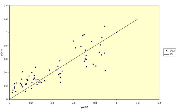
2.1.3 The “Fit” of our augmented model

I reproduced Jones [2002] figure 3.1 with g+d= 0.05 into the following figure (for extensive explanation of the derivation see the Appendix C):

(10)

Figure 1 0 0.2 0.4 0.6 0.8 1 1.2 1.4 0 0.2 0.4 0.6 0.8 1 1.2 1.4 yrel97 y/ yu s _y/yus 45°

As can be seen in the figure, Jones´ augmented Solow model fits pretty well with the empirical evidence. On the X-axis the GDP per worker relative to the United States is stated and on the Y-axis, the GDP per worker relative to the United States as predicted by Jones´ augmented Solow model. On the 45° line, the predicted value is equal to the observed value.

I also reproduced Jones [2002] figure 3.1 with g+d= 0.075 into the following figure (for extensive explanation of the derivation see the Appendix C):

Figure 2 0 0.2 0.4 0.6 0.8 1 1.2 1.4 0 0.2 0.4 0.6 0.8 1 1.2 1.4 Yrel97 y/ yu s _{yrel97 y/yus} Series2

(11)

In order to compare the estimations with the predicted model of Jones, I also have used g+d=0.075. One can conclude that with our estimated values for α, 0.40, and ψ, 0.17, the predicted GDP per worker relative to the United States, fits better with the empirical evidence than α, 0.30, and ψ, 0.10, as predicted by Jones. The distribution of my plot is better situated around the 45° line. Only for the rich countries, the values predicted by Jones, lead to a better fit with the empirical evidence. As can be seen, my results contrast significantly with the figure as depicted in Jones. The reason for that is that I run a regression, hence estimating the coefficients, whilst Jones uses the method of imputation, claiming that α and ψ should have certain values.

2.2 Convergence Regressions 2.2.1 Unconditional Convergence

The underlying equation used to make the equation for the convergence estimation is the following:

( )

(

1

) ( )

ln * ln

( )

0 ln y e t y e t y t λ λ − − ₊ − =

With some algebra (see appendix A) we get to equation B1: (B1) ln

( )

yt −ln

( )

y₀ =β₀+β₁ln

( )

y₀

Running a regression in Eviews we get to the following table (we also included the numbers of the tables in Mankiw, Romer and Weil, in order to compare them):

Unconditional convergence Table V

MRW: log difference GDP per working-age person 1960-1985 Own: log difference GDP per worker 1960-1997

Observations 75 64 22 21 β0 Constant 0.587 1.138 3.69 6.23 (0.433) (0.689) (0.68) (0.707) β1 ln(Y60) ln(Y60) -0.00423 -0.043 -0.341 -0.570 (0.05484) (0.079) (0.079) (0.075) R² (adj.) -0.01 -0.011 0.46 0.737 s.e.e. 0.41 0.515 0.18 0.189 Implied λ 0.00017 0.0012 0.0167 0.022 (0.00218) (0.0023) (0.0022) (0.0022) (0.0048) (0.0045)

Looking at the results of our estimation, we can conclude that there is no evidence for worldwide unconditional convergence. For the intermediate sample, the coefficient β1 is insignificant and the adj. R2 is very low. The starting point, GDP per worker in 1960, does not explain the worldwide differences in growth. For the OECD sample, there is evidence for unconditional convergence. The β1 coefficient is strongly significant and the adj. R2_{is very high. This phenomenon can also be seen in Sala-I-Martin} [1996]. Therefore one can conclude that there is only evidence for unconditional convergence in groups

(12)

of similar countries or regions, with a similar steady state but not for convergence in the whole world. The predicted speed of converges, the implied λ, for the OECD group is about 2%, this implies a halfway time of about 35 years. One can ignore the intermediate sample in this case, because one already has concluded that there was no evidence for convergences in this sample.

If I compare the results with the results of the MRW model, the most important difference is the adj. R2 for OECD countries. In my estimation, the adj. R2_{is 0.28 higher than in the MRW model. This difference} could be caused by the fact that the depending variable is different. Due to differences between countries in unemployment, retirements etc. the working-age population can differ significantly from the worker population. This therefore will influence the results of the estimation.

2.2.2 Conditional Convergence in the basic Solow model

The underlying equation used to make the estimation for conditional convergence in the original Solow model is the following:

( )

(

) ( )

( )

0 * ln ln 1 ln y e t y e t y t λ λ − − ₊ − =

With some algebra (see appendix A) we get to equation B2i:

(B2i) ln

( )

y_t −ln

( )

y₀ =β₀+β₁ln

( )

y₀ +β₂ln

( )

s_k +β₃ln

(

n−g−d

)

+ε

Conditional convergence, basic Solow model Table VI

Observations 75 64 22 21 β0 Constant 2.23 2.02 2.19 2.644 (0.86) (1.12) (1.17) (1.333) β1 ln(Y60) ln(Y60) -0.228 -0.353 -0.351 -0.5612 (0.057) (0.077) (0.066) (0.0598) β2 ln(I/GDP) ln(sk) 0.644 0.688 0.392 0.3788 (0.104) (0.121) (0.176) (0.2084) β3 ln(n+g+δ) ln(n+g+d) -0.464 -1.116 -0.753 -1.4079 (0.307) (0.4229) (0.341) (0.4179) R² (adj.) 0.35 0.4348 0.62 0.83497 s.e.e. 0.33 0.3851 0.15 0.15 implied λ 0.0104 0.0115 0.0173 0.0217 (0.0019) (0.0019) (0.0030) (0.0031) (0.0041) (0.0036)

Looking at the results of our estimation, one can see that there is evidence for conditional convergence between countries. The adj. R2_{is pretty good for the intermediate countries and very high for the OECD}

(13)

sample. More than 83% of the differences in growth rates between OECD countries can be explained by differences in 3 factors; the starting point, GDP per worker in 1960, the savings rate and the population growth. For the intermediate sample this is more than 43%. This means that besides the 3 factors already mentioned, there should more that explains the global differences in growth rates between countries. The speed of convergence, the implied λ, is approximately 1% for the intermediate sample and 2% for the OECD sample. This is much lower than the 4% predicted by the Solow model. The half way time for the OECD countries therefore should be about 35 years instead of the 17 years predicted by the Solow model Compared with the MRW model, the only real difference is the adj. R2_{for the OECD sample. In our} model, the adj. R2_{is more than 0.2 higher, this means that the model explains over 20% more in the} differences between growth in the OECD countries. As in the case of unconditional convergence, this can be caused by the difference in the dependent variable.

The restriction imposed on equation B2i is the following:

2 3 3

2 β 0 β β

β + = → =−

This restriction leads us to equation B2ii:

(B2ii) ln

( )

yt −ln

( )

y0 =β0+β1ln

( )

y0 +β2

(

ln

( )

sk −ln

(

n+g+d

)

+ε

Conditional convergence, basic Solow model, restricted Table VII

Observations 75 64 22 21 β0 Constant 2.90 5.37 (0.57) (0.7145) β1 ln(Y60) -0.3266 -0.561 (0.0714) (0.0668) β2 ln(sk)-ln(n+g+d) 0.7429 0.5460 (0.1048) (0.2186) R² (adj.) 0.436 0.7942 s.e.e. 0.3846 0.1676 Test of restriction: p-value 0.3666 0.0321 implied λ 0.0104 0.0217 (0.0028) (0.0040) implied α 0.6946 0.4932 (0.0034) (0.0108)

I wanted to check whether the implied α in this model was similar to the predicted α by the Solow model. In order to calculate our implied α, I restricted our model, to a model with only one coefficient that

(14)

includes α. The implied α in the intermediate, 0.69, and the OECD sample, 0.49 is too large for the Solow model. The p-value of our restriction is very low. One therefore has to reject the hypothesis β2 + β3=0. Because this was one of the four necessary characteristics of the model, the conclusion is that the Solow model fails in explaining the differences in growth between countries.

2.2.3 Conditional Convergence in the augmented model

The underlying equation used to make the estimation for the convergence in the augmented Solow model is the following:

( )

(

) ( )

( )

0 * _ln ln 1 ln y e t y e t y t λ λ − − ₊ − =

With some algebra (see appendix A) we get to equation B3i:

(B3i) ln

( )

yt −ln

( )

y0 =β0+β1ln

( )

y0 +β2ln

( )

sk +β3ln

(

n−g−d

)

+β4u+ε

Conditional convergence, augmented Solow model Table VIII

MRW Own MRW Own MRW Own

Observations 75 64 22 21 β0 Constant 3.69 2.371 2.81 2.747 (0.91) (1.17) (1.19) (1.365) β1 ln(Y60) ln(Y60) -0.366 -0.411 -0.398 -0.613 (0.067) (0.0956) (0.070) (0.998) β2 ln(I/GDP) ln(sk) 0.538 0.6119 0.335 0.3446 (0.102) (0.142) (0.174) (0.2183) β3 ln(n+g+δ) ln(n+g+d) -0.551 -1.0291 -0.844 -1.4634 (0.288) (0.4311) (0.334) (0.4335) β4 ln(SCHOOL) u 0.271 0.0368 0.223 0.0189 (0.081) (0.0360) (0.144) (0.0288) R² (adj.) 0.43 0.4353 0.65 0.8292 s.e.e. 0.30 0.3849 0.15 0.1526 implied λ 0.0182 0.0139 0.0203 0.025 (0.0020) (0.0020) (0.0042) (0.0043) (0.0047) (0.0679) implied ψ 0.0895 0.0308 (0.0059) (0.0026)

The signs for this estimation coefficients are the ones we expected. Convergence should indeed depend positively on savings and education and negatively from y(0) and population growth. However, for the intermediate set β4 is not significant and for the OECD set only β3 is significant. Remarkably, for the latter

(15)

set I get an extraordinary high adjusted R², which suggests that the overall explanatory power of the Jones Model is better than that of MRW. The implied ψ estimated by the regression differs in the OECD case substantially from the 0.10 suggested by Jones. However, to reject the 0.10 null-hypothesis we should have run a significance test for ψ = 0.10. Interestingly, the standard errors of the implied λ reported by MRW are both to high, as compared to those estimated by us using the formula mentioned in the appendix.

The restriction imposed on equation B3i is the following:

2 3 3

2 β 0 β β

β + = → =−

This restriction leads us to equation B3ii:

(B3ii) ln

( )

y_t −ln

( )

y₀ =

β

₀+

β

₁ln

( )

y₀ +

β

₂

(

ln

( )

s_k −ln

(

n+g+d

)

+

β

₄u+

ε

Conditional convergence, augmented Solow model, restricted Table IX

Observations 75 64 22 21 β0 Constant 3.09 3.2352 3.55 5.3527 (0.53) (0.6535) (0.63) (0.9255) β1 ln(Y60) ln(Y60) -0.372 -0.3860 -0.402 -0.5577 (0.067) (0.0913) (0.069) (0.1096) β2 ln(I/GDP)-ln(n+g+δ) ln(sk)-ln(n+g+d) 0.506 0.6639 0.396 0.5472 (0.095) (0.1292) (0.152) (0.2272) β3 ln(SCHOOL)-ln(n+g+δ) u 0.266 0.0375 0.236 -0.0012 (0.08) (0.0359) (0.141) (0.0311) R² (adj.) 0.44 0.4373 0.66 0.7821 s.e.e. 0.30 0.3843 0.15 0.1724 Test of restriction: p-value 0.42 0.3781 0.47 0.0297 implied λ 0.0186 0.0128 0.0206 0.0125 (0.0019) (0.0020) (0.0043) (0.0039) (0.0046) (0.0065) implied α 0.44 0.6324 0.38 0.4952 (0.07) (0.0051) (0,13) (0.0127) implied β 0.23 0.23 (0.06) (0,11) implied ψ 0.0971 -0.0021 (0.0439) (0.0551)

(16)

Imposing the restriction that the effects of β2 and β3 of Table VIII should complement themselves to zero we get an interesting picture. Whereas the p-value of the intermediate set, totally in line with MRW, indicates that the restriction is legitimate, the very low value in the OECD sample gives highly significant evidence to reject the hypothesis. These results for the implied α are both higher than in MRW. Again, the standard errors for the implied λ are more than twice as high as what MRW reports. My estimate for the implied ψ is very close to the 0.10 suggested by Jones for the intermediate countries yet even negative, although insignificant, for the OECD set.

(17)

3. Conclusion

Concerning the level regressions, MRW conclude that adding human capital to the Solow model improves its performance. I can certainly state the same result. Most obviously, the adjusted R2_increases visibly in the augmented version. Further, the implied α decreases to a value which is closer to 1_/

3. I also reduced an omitted variable bias which had made the coefficient on saving of the basic Solow model too high. However, whilst I only had to reject the restriction in the basic model for the Intermediate set, we rejected the restrictions for both sets after the augmentation, implying that in the augmented model the effects of savings and population growth did not complement each other.

Refering to the convergence debate MRW state that the basic Solow model does not predict absolute convergence but certainly predicts conditional convergence. These results are supported by my estimations, too. Surprisingly, the standard errors for the implied λ stated by MRW are wrong throughout all convergence tables. Yet, whereas the addition of human capital makes a sensible contribution in the MRW model, in my estimation the coefficients of u are never significant in the convergence regressions. Moreover, the Jones model also fails to produce a reasonable value for the implied α.

It is worth pointing out some problems related with these estimates of conditional convergence rates, as mentioned in Klenow et al. [1997]. First, regressions usually include control variables that are related to steady-state income and to transition dynamics. This makes it difficult to say whether the order if magnitude of the coefficient on initial income picks up all the transitory dynamics in the model. Secondly, these models don’t point to observable control variables that can fully capture differences in steady-states. In more recent empirical analysis, some other authors use country fixed effects in panel regressions in order to control for differences in steady-states and in fact they get higher convergence speed rates.

(18)

4 Appendices A. Formula Sheet A1i (level, basic)

Steady state output per worker basic Solow model

(

)

( ) t k t t _A d g n s L Y ⋅ + + = −α α 1 * Regression equation

( ) ( ) ( ) ( ) (

)

( )

₍

_{) ( ) (}

_{) (}

)

( )

(

) ( ) (

) (

)

( )

β

(

)

ε β β ε α α α α ε α α α α α α α α + + + − + = ⎟⎟ ⎠ ⎞ ⎜⎜ ⎝ ⎛ + + + − − − + = ⎟⎟ ⎠ ⎞ ⎜⎜ ⎝ ⎛ + = + + + − − − + + = ⎟⎟ ⎠ ⎞ ⎜⎜ ⎝ ⎛ + + − − − + = ⎟⎟ ⎠ ⎞ ⎜⎜ ⎝ ⎛ d g n s L Y d g n s a L Y a g A d g n s g A L Y d g n s A L Y k t t k t t t k t t t k t t t ln ln ln ln 1 ln 1 ln ln ln 1 ln 1 ln ln ln 1 ln 1 ln ln 2 1 0 * * 0 0 * *

A1ii (level, basic, restricted) Regression equation

( )

(

)

( )

(

)

(

)

(

) ( )

(

)

(

)

(

1₁

)

1 * 1 0 * 1 1 0 * 1 2 2 1 ˆ 1 ˆ ˆ ˆ 1 ˆ ˆ ln ln 1 ln ln ln ln ln ln ln 0 β β α α α β ε α α ε β β ε β β β β β β β + = → − = + + + − − + = ⎟⎟ ⎠ ⎞ ⎜⎜ ⎝ ⎛ + + + − + = ⎟⎟ ⎠ ⎞ ⎜⎜ ⎝ ⎛ + + + − + = ⎟⎟ ⎠ ⎞ ⎜⎜ ⎝ ⎛ − = ⇔ = + d g n s a L Y d g n s L Y d g n s L Y k t t k t t k t t Standard Error

α

ˆ

Taylor approximation

(

) (

)

(

)

(

) (

)

(

)

(

)

(

) (

)

( ) ( ) ( )

(

)

( )

(

*

)

2

( )

1 1 1 4 * 1 2 2 * 1 * 1 * 1 * 1 1 2 * 1 2 * 1 * 1 1 2 * 1 * 1 * 1 * 1 1 2 * 1 * 1 * 1 ˆ 1 1 ˆ ˆ 1 1 1 1 ˆ 1 1 ˆ 1 ˆ 1 1 1 ˆ ˆ 1 1 1 ˆ β β α β β β β β β β β α β β β β β β α β β β β β α se se Var b x a Var x Var a b x a Var ⋅ + = ⋅ − = + ⋅ ⋅ = + ⋅ + − + + ⋅ + ≈ + − ⋅ + + + ≈ − ⋅ + + + ≈

(19)

A2i (level, augmented)

Steady state output per worker augmented Solow model

( ) ( ) u u t k t t e L H h L e H A h d g n s L Y ⋅ ⋅ − = = = ⋅ ⋅ + + = ψ ψ α α 1 * Regression equation

( ) ( ) ( ) ( ) (

)

( )

₍

_{) ( ) (}

_{) (}

)

( )

(

) ( ) (

) (

)

( )

(

)

ψ β ε β β β β ε ψ α α α α ε ψ α α α α α α α α ˆ ˆ ln ln ln ln 1 ln 1 ln ln ln 1 ln 1 ln ln ln ln 1 ln 1 ln ln 3 3 2 1 0 * * 0 0 * * = + + + + − + = ⎟⎟ ⎠ ⎞ ⎜⎜ ⎝ ⎛ + ⋅ + + + − − − + = ⎟⎟ ⎠ ⎞ ⎜⎜ ⎝ ⎛ + = + ⋅ + + + − − − + + = ⎟⎟ ⎠ ⎞ ⎜⎜ ⎝ ⎛ + + + − − − + = ⎟⎟ ⎠ ⎞ ⎜⎜ ⎝ ⎛ u d g n s L Y u d g n s a L Y a g A u d g n s g A L Y h d g n s A L Y k t t k t t t k t t t k t t t

A2ii (level, augmented, restricted) Regression equation ( ) ( ) ( ) ( ) ( ) ( ) ( )( ( )) ( )

( )

ψ β β β α α α β ε ψ α α ε β β β ε β β β β β β β β ˆ ˆ ˆ 1 ˆ ˆ ˆ 1 ˆ ˆ ln ln 1 ln ln ln ln ln ln ln 0 3 1 1 1 * 3 1 0 * 3 1 1 0 * 1 2 2 1 = + = ⇔ − = + ⋅ + + + − − + = ⎟⎟ ⎠ ⎞ ⎜⎜ ⎝ ⎛ + + + + − + = ⎟⎟ ⎠ ⎞ ⎜⎜ ⎝ ⎛ + + + + − + = ⎟⎟ ⎠ ⎞ ⎜⎜ ⎝ ⎛ − = → = + u d g n s a L Y u d g n s L Y u d g n s L Y k t t k t t k t t Standard error

α

ˆ

(

)

( )

(

_{) (}

₎

₍

₎

(

)

(

) (

)

(

)

( )

(

)

₍

₎

( )

(

*

)

2

( )

1 1 1 4 * 1 2 2 * 1 * 1 * 1 * 1 1 2 * 1 2 * 1 * 1 1 2 * 1 * 1 * 1 ˆ 1 1 ˆ ˆ 1 1 1 1 ˆ 1 1 ˆ 1 ˆ 1 1 1 ˆ β β α β β β β β β β β α β β β β β β α se se Var b x a Var x Var a b x a Var x se a b ax se ⋅ + = ⋅ − = + ⋅ ⋅ = + ⋅ + − + + ⋅ + ≈ + − ⋅ + + + ≈ ⋅ = +

(20)

B1 (unconditional convergence) Regression equation

( )

(

) ( )

( )

(

) ( ) (

)

( )

(

)

( )

t e y y y gt A y e y e y y gt A y e y e y t t t t t t t t − + = → − − = + = − + + − − − = − + + + − = − − − − − 1 ˆ ln ˆ 1 ˆ ln ln ln ) 0 ( ln 1 ln 1 ln ln ) 0 ( ln ln 1 ln 1 1 0 1 0 0 0 * 0 0 * β λ β β β λ λ λ λ λ Standard error

λ

ˆ

( )

βˆ1 =₋1 ⋅

(

ln

(

βˆ1+1

)

λ t

Taylor Approximation around β1*:

( )

(

)

₍

₎

(

)

( )

(

)

₍

₎

₍

₎

( )

₍

₎

( )

₍

*

₎

( )

1 1 1 * 1 1 * 1 * 1 * 1 1 * 1 1 * 1 1 * 1 * 1 1 ˆ 1 1 ˆ 1 1 ˆ 1 1 ˆ 1 ln ˆ ˆ 1 1 1 1 ln ˆ β β β β β λ β β β β β β λ β β β β β λ se t c ax se C t t t t t t ⋅ + − = + + ⋅ + − ≈ + − − + − + − + ≈ − ⋅ + ⋅ − + − + ≈

B2i (conditional convergence, basic Solow) Regression equation

( )

(

) ( )

( )

(

) ( ) (

)

( )

(

)

( )

(

)

₍

₎

( )

(

)

( )

(

)

( )

(

)

(

)

(

)

( )

(

)

(

)

(

)

t e d g n s y y y gt A y e d g n e s e y y gt A y e d g n s e y y d g n s y gt A y e y e y y gt A y e y e y t k t t t k t t t k t t k t t t t t t − + = ⇔ − − = + − − + + + = − + + − − + + ⎟ ⎠ ⎞ ⎜ ⎝ ⎛ − − − ⎟ ⎠ ⎞ ⎜ ⎝ ⎛ − − = − + + − − ⎟ ⎟ ⎠ ⎞ ⎜ ⎜ ⎝ ⎛ + + − = − + + = + + − − − = − + + + − = − − − − − − − − − − − − 1 ˆ ln ˆ 1 ˆ ln ln ln ln ln ) 0 ( ln 1 ln 1 1 ln 1 1 ln ln ) 0 ( ln 1 ln 1 ln ln ) 0 ( ln 1 ln 1 ln ln ) 0 ( ln ln 1 ln 1 1 3 2 0 1 0 0 0 0 0 1 0 1 * 0 * 0 0 * β λ β ε β β β β α α α α λ λ λ λ λ α α λ α α λ λ λ λ Standard error

λ

ˆ

( )

ˆ₁ 1 ⋅

(

ln

(

ˆ₁+1

)

− = β β λ t

( )

(

)

₍

₎

(

)

( )

(

)

₍

₎

₍

₎

( )

₍

₎

(

)

₍

*

₎

( )

(21)

B2ii (conditional convergence, basic Solow, restricted) Regression equation ( ) ( ) ( ) ( ) ( ) ( ) ( ) ( ) ( ( ) ( )) ( ) ( )

(

)

( ( ) ( ))

(

)

( )

(

)

(

)

(

)

1 2 2 1 2 2 1 1 0 0 2 0 1 0 0 2 2 0 1 0 0 2 3 3 2 ˆ ˆ ˆ ˆ ˆ ˆ ˆ 1 ˆ 1 1 ˆ 1 ˆ ln ˆ 1 ˆ ) 0 ( ln 1 ln ln 1 1 ln ln ln ln ln ln ln ln ln ln ln ln 0 β β β β β β β λ β α α ε β β β ε β β β β β β β β λ λ λ -α -α α α α e t e gt A y e d g n s e y y d g n s y y y d g n s y y y λt t t k t t k t k t = ⇔ = ⎟ ⎠ ⎞ ⎜ ⎝ ⎛ − ⇔ ⎟ ⎠ ⎞ ⎜ ⎝ ⎛ − − = − + = ⇔ − − = + + − − + + − ⎟ ⎠ ⎞ ⎜ ⎝ ⎛ − − = − + + + − + + = − + + + − + + = − − = ⇔ = + − − − − Standard error

λ

ˆ

( )

ˆ1 1 ⋅

(

ln

(

ˆ1+1

)

− = β β λ t

( )

(

)

₍

₎

(

)

( )

(

)

₍

₎

₍

₎

( )

₍

₎

(

)

₍

*

₎

( )

1 1 1 * 1 1 * 1 * 1 * 1 1 * 1 1 * 1 1 * 1 * 1 1 ˆ 1 1 ˆ 1 1 ˆ 1 1 ˆ 1 ln ˆ ˆ 1 1 1 1 ln ˆ β β β β β λ β β β β β β λ β β β β β λ se t c ax se C t t t t t t ⋅ + − = + + ⋅ + − ≈ + − − + − + − + ≈ − ⋅ + ⋅ − + − + ≈ Standard error

α

ˆ

( ) (₍ )₎ ₍ ₎ ( ) ( ) ₍ ₎

(

)

₍

_{) (}

₎

(

)

₍

₎

(

)

(

)

₍

_{) (}

₎

₍

₎

( ) ( ) ( ) ( ) ( )

₍

₎

( )

₍

₎

( )

₍

_*

₎

4

(

2 1

)

1 * 2 * 2 * 1 1 4 * 1 * 2 2 * 2 2 4 * 1 * 2 2 * 1 2 2 1 2 * 1 * 2 * 2 2 2 * 1 * 2 * 1 * 1 * 2 * 2 1 2 * 1 1 2 * 1 * 2 * 2 * 2 2 2 * 1 * 2 * 1 * 1 * 2 * 2 1 2 2 1 2 2 2 1 2 2 1 2 ' 2 2 1 2 1 2 1 2 2 1 2 1 2 ' 1 1 2 2 ˆ , ˆ 2 ˆ . ˆ , 2 . ˆ ˆ ˆ , ˆ ˆ ˆ ˆ ˆ , ˆ ˆ 1 1 , 1 1 , β β β β β β β β β β β β β β β β β β β β β β β β β β β α β β β β β β β β β β β β β β β α β β β β β β β β α β β β β β β β β β β α β β β α Cov Var Var by ax Var y x Cov ab y Var b x Var a by ax Var − ⋅ ⋅ − − + ⋅ − = + ⋅ + + ⋅ = + ⋅ − + ⋅ − − + − ≈ − ⋅ − + − ⋅ − − + − ≈ − − = − ⋅ − ⋅ ⋅ − = − − = − ⋅ − − ⋅ = − = −

B3i (conditional convergence, augmented Solow) Regression equation

(22)

( )

(

) ( )

( ) ( ) ( )

(

) ( ) (

)

( ) ( ) ( ) ( ) ( )

(

)

₍ ₎ ( )

(

)

( ) ( ) ( )

(

)

( )

(

)

( )

(

)

(

)

( ) ( ) ( ) ( ) ( ) ( )

( )

(

)

1 4 4 1 1 4 3 2 0 1 0 0 0 0 0 1 0 1 * 0 * 0 0 * ˆ ˆ ˆ 1 ˆ 1 ˆ ln ˆ ˆ ln ln ln ln ln ln 1 1 ln 1 1 ln 1 1 ln ln ln 1 ln 1 ln ln ln 1 ln 1 ln ln ln ln 1 ln β β ψ ψ β β λ β ε β β β β β ψ α α α α λ λ λ λ λ λ λ α α λ α α λ λ λ λ = ⇒ − − = − + = ⇒ − = + + − − + + + = − − − ⋅ − + + + ⎟ ⎠ ⎞ ⎜ ⎝ ⎛ − − − ⎟ ⎠ ⎞ ⎜ ⎝ ⎛ − − = − − − ⎟ ⎟ ⎠ ⎞ ⎜ ⎜ ⎝ ⎛ ⋅ + + − = − + + = − − − = − + − = − − − − − − − − − − − − − − t t k t t t t k t t t k t t k t t t t t t e t e u d g n s y y y y e u e d g n e s e y y y e h d g n s e y y h d g n s y y e y e y y y e y e y Standard error

λ

ˆ

( )

ˆ₁ 1 ⋅

(

ln

(

ˆ₁+1

)

− = β β λ t

( )

(

)

₍

₎

(

)

( )

(

)

₍

₎

₍

₎

( )

₍

₎

(

)

₍

*

₎

( )

1 1 1 * 1 1 * 1 * 1 * 1 1 * 1 1 * 1 1 * 1 * 1 1 ˆ 1 1 ˆ 1 1 ˆ 1 1 ˆ 1 ln ˆ ˆ 1 1 1 1 ln ˆ β β β β β λ β β β β β β λ β β β β β λ se t c ax se C t t t t t t ⋅ + − = + + ⋅ + − ≈ + − − + − + − + ≈ − ⋅ + ⋅ − + − + ≈ Standard error

ψ

ˆ

( ) ( ) ₂ 1 4 1 4 ' 2 1 1 4 ' 1 1 4 , 1 , ˆ β β β β ψ β β β ψ β β ψ = − = − =

Taylor Approximation around β1* and β4*:

(

)

(

)

(

)

(

)

(

)

(

)

( )

(

)

( )

*3

(

4 1

)

1 * 4 1 4 * 1 2 * 4 4 2 * 1 2 2 1 2 * 1 * 4 4 * 1 1 4 1 2 * 1 * 4 4 * 1 * 1 * 4 1 4 * 1 1 2 * 1 * 4 * 4 4 * 1 * 1 * 4 1 4 ˆ , ˆ 2 ˆ ˆ 1 , 2 ˆ ˆ 1 , ˆ ˆ 1 , ˆ ˆ 1 , β β β β β β β β β β β β β β β β ψ β β β β β β β β β ψ β β β β β β β β β β β ψ Cov Var Var by ax Var y x Cov ab y Var b x Var a by ax Var C ⋅ ⋅ − ⋅ + ⋅ = + ⋅ + ⋅ + ⋅ = + + ⋅ + ⋅ − ≈ ⋅ + ⋅ − + − ≈ − + − ⋅ − + − ≈

(23)

B3ii (conditional convergence, augmented Solow, restricted) Regression equation

( )

(

)

( )

(

( )

(

)

( )

(

)

(

( )

(

)

(

)

(

)

( )

(

)

(

)

(

)

(

)

1 4 4 1 2 2 1 2 2 1 1 0 0 4 2 0 1 0 0 4 2 2 0 1 0 0 2 3 3 2 ˆ ˆ ˆ 1 ˆ ˆ ˆ ˆ ˆ ˆ ˆ 1 ˆ 1 1 ˆ 1 ˆ ln ˆ 1 ˆ ln 1 1 ln ln 1 1 ln ln ln ln ln ln ln ln ln ln ln ln 0 β β ψ ψ β β β β β β β β λ β ψ α α ε β β β β ε β β β β β β β β β λ λ λ λ λ = ⇒ − − = = ⇔ = ⎟ ⎠ ⎞ ⎜ ⎝ ⎛ − ⇔ ⎟ ⎠ ⎞ ⎜ ⎝ ⎛ − − = − + = ⇒ − − = − − − + + + − ⎟ ⎠ ⎞ ⎜ ⎝ ⎛ − − = − + + + + − + + = − + + + + − + + = − − = ⇔ = + − − − − − − t λt t t t t t k t k t e -α -α α α α e t e y e u e d g n s e y y u d g n s y y y u d g n s y y y Standard error

α

ˆ

( ) ( ) ( ) ( ) ( ) ( ) ( )2 1 2 2 2 1 2 2 1 2 ' 2 2 1 2 1 2 1 2 2 1 2 1 2 ' 1 1 2 2 ) 1 ( ) 1 ( , 1 1 , β β β β β β β β α β β β β β β β β β β α β β β α − = − ⋅ − ⋅ ⋅ − = − − = − ⋅ − − ⋅ = − = −

(

)

₍

_{) (}

₎

(

)

₍

₎

(

)

(

)

₍

_{) (}

₎

₍

₎

(

)

( )

(

)

(

)

( )

(

)

( )

(

*

)

4

(

2 1

)

1 * 2 * 2 * 1 1 4 * 1 * 2 2 * 2 2 4 * 1 * 2 2 * 1 2 2 1 2 * 1 * 2 * 2 2 2 * 1 * 2 * 1 * 1 * 2 * 2 1 2 * 1 1 2 * 1 * 2 * 2 * 2 2 2 * 1 * 2 * 1 * 1 * 2 * 2 1 2 ˆ , ˆ 2 ˆ . ˆ , 2 . ˆ ˆ ˆ , ˆ ˆ ˆ ˆ ˆ , ˆ ˆ β β β β β β β β β β β β β β β β β β β β β β β β β β β α β β β β β β β β β β β β β β β α Cov Var Var by ax Var y x Cov ab y Var b x Var a by ax Var − ⋅ ⋅ − − + ⋅ − = + ⋅ + + ⋅ = + ⋅ − + ⋅ − − + − ≈ − ⋅ − + − ⋅ − − + − ≈ Standard error

λ

ˆ

( )

βˆ1 =₋1 ⋅

(

ln

(

βˆ1+1

)

λ t

( )

(

)

₍

₎

(

)

( )

(

)

₍

₎

₍

₎

( )

₍

₎

( )

₍

*

₎

( )

(24)

Standard error

ψ

ˆ

( ) ( ) 2 1 4 1 4 ' 2 1 1 4 ' 1 1 4 , 1 , ˆ β β β β ψ β β β ψ β β ψ = − = − =

( )

(

)

(

)

( ) ( ) ( ) ( ) ( ) ( ) ( )

( )

*3

(

4 1

)

1 * 4 1 4 * 1 2 * 4 4 2 * 1 2 2 1 2 * 1 * 4 4 * 1 1 4 1 2 * 1 * 4 4 * 1 * 1 * 4 1 4 * 1 1 2 * 1 * 4 * 4 4 * 1 * 1 * 4 1 4 ˆ , ˆ 2 ˆ ˆ 1 , 2 ˆ ˆ 1 , ˆ ˆ 1 , ˆ ˆ 1 , β β β β β β β β β β β β β β β β ψ β β β β β β β β β ψ β β β β β β β β β β β ψ Cov Var Var by ax Var y x Cov ab y Var b x Var a by ax Var C ⋅ ⋅ − ⋅ + ⋅ = + ⋅ + ⋅ + ⋅ = + + ⋅ + ⋅ − ≈ ⋅ + ⋅ − + − ≈ − + − ⋅ − + − ≈

(25)

B. Eviews Output

Intermediate countries

Equation A1i

Dependent Variable: LOG(Y97) Method: Least Squares Sample: 1 64

Included observations: 64

Variable Coefficient Std. Error t-Statistic Prob.

C 3.321580 1.624237 2.045010 0.0452

LOG(SK) 0.952227 0.170453 5.586458 0.0000

LOG(N+0.05) -2.871358 0.535917 -5.357842 0.0000

R-squared 0.650496 Mean dependent var 9.419161

Adjusted R-squared 0.639037 S.D. dependent var 0.935650

S.E. of regression 0.562141 Akaike info criterion 1.731613

Sum squared resid 19.27615 Schwarz criterion 1.832810

Log likelihood -52.41161 F-statistic 56.76644

Durbin-Watson stat 1.058312 Prob(F-statistic) 0.000000

Wald Test: Equation: A1I Null Hypothesis: C(2)+C(3)=0 F-statistic 9.148874 Probability 0.003639 Chi-square 9.148874 Probability 0.002489 Equation A1ii

C 8.216904 0.145786 56.36269 0.0000

LOG(SK)-LOG(N+0.05) 1.296460 0.134976 9.605113 0.0000

Equation A2i

C 4.372902 1.432638 3.052343 0.0034

(26)

LOG(N+0.05) -1.766416 0.526381 -3.355772 0.0014

U 0.167314 0.036935 4.529929 0.0000

C 7.532087 0.182207 41.33801 0.0000

LOG(SK)-LOG(N+0.05) 0.655328 0.169725 3.861106 0.0003

U 0.187986 0.036880 5.097242 0.0000

Equation B1

Dependent Variable: LOG(Y97)-LOG(Y60) Method: Least Squares

Sample: 1 64

C 1.137633 0.688795 1.651628 0.1037

LOG(Y60) -0.042946 0.079252 -0.541887 0.5898

Adjusted R-squared -0.011339 S.D. dependent var 0.512247 S.E. of regression 0.515143 Akaike info criterion 1.542006

(27)

Sample: 1 64

C 2.023663 1.123458 1.801281 0.0767

LOG(Y60) -0.353290 0.077307 -4.569934 0.0000

LOG(SK) 0.688212 0.120959 5.689608 0.0000

LOG(N+0.05) -1.115580 0.422893 -2.637974 0.0106

Wald Test: Equation: B2I Null Hypothesis: C(3)+C(4)=0 F-statistic 0.827464 Probability 0.366647 Chi-square 0.827464 Probability 0.363007 Equation B2ii

Sample: 1 64

C 2.903171 0.571320 5.081516 0.0000

LOG(Y60) -0.326598 0.071421 -4.572857 0.0000

LOG(SK)-LOG(N+0.05) 0.742928 0.104795 7.089355 0.0000

Equation B3i

Sample: 1 64

C 2.370646 1.173092 2.020853 0.0478

LOG(Y60) -0.410955 0.095642 -4.296811 0.0001

(28)

LOG(N+0.05) -1.029091 0.431093 -2.387167 0.0202

U 0.036803 0.035965 1.023293 0.3103

Wald Test: Equation: B3I Null Hypothesis: C(3)+C(4)=0 F-statistic 0.788694 Probability 0.378101 Chi-square 0.788694 Probability 0.374495 Equation B3ii

Sample: 1 64

C 3.235163 0.653457 4.950845 0.0000

LOG(Y60) -0.385974 0.091251 -4.229819 0.0001

LOG(SK)-LOG(N+0.05) 0.663906 0.129200 5.138609 0.0000

U 0.037481 0.035894 1.044216 0.3006

(29)

We used the following correlation matrices to calculate the standard errors of the implied α, λ, and ψ: Covariance Matrix B2ii

C LOG(Y60) LOG(SK)-LOG(N+0.05)

C 0,32641 -0,04025 0,026098

LOG(Y60) -0,0403 0,0051 -0,004193

LOG(SK)-LOG(N+0.05) 0,0261 -0,00419 0,010982

Covariance Matrix B3i

C LOG(Y60) LOG(SK) LOG(N+0.05) U

C 1,376145 -0,031093 0,05899 0,398286 0,012195

LOG(Y60) -0,031093 0,009147 0,00176 0,01145 -0,002027

LOG(SK) 0,058985 0,001763 0,02018 0,007317 -0,002681

LOG(N+0.05) 0,398286 0,01145 0,00732 0,185841 0,00304

U 0,012195 -0,002027 -0,00268 0,00304 0,001293

Covariance Matrix B3ii

C LOG(Y60) LOG(SK)-LOG(N+0.05) U

C 0,427006 -0,05827 0,002 0,011412

LOG(Y60) -0,05827 0,008327 0,000116 -0,002041

LOG(SK)-LOG(N+0.05) 0,002 0,000116 0,016693 -0,002716

(30)

OECD countries

Equation A1i

Dependent Variable: LOG(Y97) Method: Least Squares Date: 03/03/05 Time: 10:00 Sample: 1 21

C 6.849169 2.386295 2.870211 0.0102

LOG(SK) 0.301400 0.412713 0.730288 0.4746

LOG(N+0.05) -1.335788 0.828478 -1.612339 0.1243

C 9.595177 0.560863 17.10788 0.0000

LOG(SK)-LOG(N+0.05) 0.469385 0.391581 1.198692 0.2454

Equation A2i

(31)

C 4.610212 1.726496 2.670272 0.0161

LOG(SK) 0.158693 0.287802 0.551397 0.5885

LOG(N+0.05) -1.699942 0.579866 -2.931611 0.0093

U 0.107440 0.023750 4.523865 0.0003

R-squared 0.608591 Mean dependent var

Adjusted R-squared 0.539519 S.D. dependent var S.E. of regression 0.206252 Akaike info criterion Sum squared resid 0.723180 Schwarz criterion Log likelihood 5.572798 F-statistic Durbin-Watson stat 0.755078 Prob(F-statistic)

C 8.791592 0.489848 17.94758 0.0000

LOG(SK)-LOG(N+0.05) 0.415064 0.305677 1.357854 0.1913

U 0.096640 0.026545 3.640633 0.0019

R-squared 0.464569 Mean dependent var

Adjusted R-squared 0.405077 S.D. dependent var S.E. of regression 0.234436 Akaike info criterion Sum squared resid 0.989280 Schwarz criterion Log likelihood 2.282943 F-statistic Durbin-Watson stat 0.834593 Prob(F-statistic)

Equation B1

Date: 03/03/05 Time: 10:03 Sample: 1 21

C 6.234026 0.707170 8.815461 0.0000

LOG(Y60) -0.569873 0.075370 -7.561003 0.0000