Introduction to the
Mathematical Theory of
Systems and Control
Plant Controller
Contents
Preface ix
1 Dynamical Systems 1
1.1 Introduction . . . 1
1.2 Models . . . 3
1.2.1 The universum and the behavior . . . 3
1.2.2 Behavioral equations . . . 4
1.2.3 Latent variables . . . 5
1.3 Dynamical Systems . . . 8
1.3.1 The basic concept . . . 9
1.3.2 Latent variables in dynamical systems . . . 10
1.4 Linearity and Time-Invariance . . . 15
1.5 Dynamical Behavioral Equations . . . 16
1.6 Recapitulation . . . 19
1.7 Notes and References . . . 20
1.8 Exercises . . . 20
2 Systems Defined by Linear Differential Equations 27 2.1 Introduction . . . 27
2.3 Constant-Coefficient Differential Equations . . . 31
2.3.1 Linear constant-coefficient differential equations . . . 31
2.3.2 Weak solutions of differential equations . . . 33
2.4 Behaviors Defined by Differential Equations . . . 37
2.4.1 Topological properties of the behavior . . . 38
2.4.2 Linearity and time-invariance . . . 43
2.5 The Calculus of Equations . . . 44
2.5.1 Polynomial rings and polynomial matrices . . . 44
2.5.2 Equivalent representations . . . 45
2.5.3 Elementary row operations and unimodular polyno-mial matrices . . . 49
2.5.4 The Bezout identity . . . 52
2.5.5 Left and right unimodular transformations . . . 54
2.5.6 Minimal and full row rank representations . . . 57
2.6 Recapitulation . . . 60
2.7 Notes and References . . . 61
2.8 Exercises . . . 61
2.8.1 Analytical problems . . . 63
2.8.2 Algebraic problems . . . 64
3 Time Domain Description of Linear Systems 67 3.1 Introduction . . . 67
3.2 Autonomous Systems . . . 68
3.2.1 The scalar case . . . 71
3.2.2 The multivariable case . . . 79
3.3 Systems in Input/Output Form . . . 83
3.4 Systems Defined by an Input/Output Map . . . 98
3.5 Relation Between Differential Systems and Convolution Sys-tems . . . 101
3.6 When Are Two Representations Equivalent? . . . 103
3.7 Recapitulation . . . 106
3.8 Notes and References . . . 107
3.9 Exercises . . . 107
4 State Space Models 119 4.1 Introduction . . . 119
4.3 State Space Models . . . 120
4.4 Input/State/Output Models . . . 126
4.5 The Behavior of i/s/o Models . . . 127
4.5.1 The zero input case . . . 128
4.5.2 The nonzero input case: The variation of the con-stants formula . . . 129
4.5.3 The input/state/output behavior . . . 131
4.5.4 How to calculateeAt? . . . 133
4.5.4.1 Via the Jordan form . . . 134
4.5.4.2 Using the theory of autonomous behaviors 137 4.5.4.3 Using the partial fraction expansion of (Iξ− A)−1 . . . 140
4.6 State Space Transformations . . . 142
4.7 Linearization of Nonlinear i/s/o Systems . . . 143
4.8 Recapitulation . . . 148
4.9 Notes and References . . . 149
4.10 Exercises . . . 149
5 Controllability and Observability 155 5.1 Introduction . . . 155
5.2 Controllability . . . 156
5.2.1 Controllability of input/state/output systems . . . . 167
5.2.1.1 Controllability of i/s systems . . . 167
5.2.1.2 Controllability of i/s/o systems . . . 174
5.2.2 Stabilizability . . . 175
5.3 Observability . . . 177
5.3.1 Observability of i/s/o systems . . . 181
5.3.2 Detectability . . . 187
5.4 The Kalman Decomposition . . . 188
5.5 Polynomial Tests for Controllability and Observability . . . 192
5.6 Recapitulation . . . 193
5.7 Notes and References . . . 194
5.8 Exercises . . . 195
6.2 Elimination of Latent Variables . . . 206
6.2.1 Modeling from first principles . . . 206
6.2.2 Elimination procedure . . . 210
6.2.3 Elimination of latent variables in interconnections . 214 6.3 Elimination of State Variables . . . 216
6.4 From i/o to i/s/o Model . . . 220
6.4.1 The observer canonical form . . . 221
6.4.2 The controller canonical form . . . 225
6.5 Canonical Forms and Minimal State Space Representations 229 6.5.1 Canonical forms . . . 230
6.5.2 Equivalent state representations . . . 232
6.5.3 Minimal state space representations . . . 233
6.6 Image Representations . . . 234
6.7 Recapitulation . . . 236
6.8 Notes and References . . . 237
6.9 Exercises . . . 237
7 Stability Theory 247 7.1 Introduction . . . 247
7.2 Stability of Autonomous Systems . . . 250
7.3 The Routh–Hurwitz Conditions . . . 254
7.3.1 The Routh test . . . 255
7.3.2 The Hurwitz test . . . 257
7.4 The Lyapunov Equation . . . 259
7.5 Stability by Linearization . . . 268
7.6 Input/Output Stability . . . 271
7.7 Recapitulation . . . 276
7.8 Notes and References . . . 277
7.9 Exercises . . . 277
8 Time- and Frequency-Domain Characteristics of Linear Time-Invariant Systems 287 8.1 Introduction . . . 287
8.2 The Transfer Function and the Frequency Response . . . . 288
8.2.1 Convolution systems . . . 289
8.2.3 The transfer function represents the controllable part
of the behavior . . . 295
8.2.4 The transfer function of interconnected systems . . . 295
8.3 Time-Domain Characteristics . . . 297
8.4 Frequency-Domain Response Characteristics . . . 300
8.4.1 The Bode plot . . . 302
8.4.2 The Nyquist plot . . . 303
8.5 First- and Second-Order Systems . . . 304
8.5.1 First-order systems . . . 304
8.5.2 Second-order systems . . . 304
8.6 Rational Transfer Functions . . . 307
8.6.1 Pole/zero diagram . . . 308
8.6.2 The transfer function of i/s/o representations . . . . 308
8.6.3 The Bode plot of rational transfer functions . . . 310
8.7 Recapitulation . . . 313
8.8 Notes and References . . . 313
8.9 Exercises . . . 314
9 Pole Placement by State Feedback 317 9.1 Open Loop and Feedback Control . . . 317
9.2 Linear State Feedback . . . 323
9.3 The Pole Placement Problem . . . 324
9.4 Proof of the Pole Placement Theorem . . . 325
9.4.1 System similarity and pole placement . . . 326
9.4.2 Controllability is necessary for pole placement . . . . 327
9.4.3 Pole placement for controllable single-input systems 327 9.4.4 Pole placement for controllable multi-input systems 329 9.5 Algorithms for Pole Placement . . . 331
9.6 Stabilization . . . 333
9.7 Stabilization of Nonlinear Systems . . . 335
9.8 Recapitulation . . . 339
9.9 Notes and References . . . 339
9.10 Exercises . . . 340
10 Observers and Dynamic Compensators 347 10.1 Introduction . . . 347
10.3 Pole Placement in Observers . . . 352
10.4 Unobservable Systems . . . 355
10.5 Feedback Compensators . . . 356
10.6 Reduced Order Observers and Compensators . . . 364
10.7 Stabilization of Nonlinear Systems . . . 368
10.8 Control in a Behavioral Setting . . . 370
10.8.1 Motivation . . . 370
10.8.2 Control as interconnection . . . 373
10.8.3 Pole placement . . . 375
10.8.4 An algorithm for pole placement . . . 377
10.9 Recapitulation . . . 382
10.10Notes and References . . . 383
10.11Exercises . . . 383
A Simulation Exercises 391 A.1 Stabilization of a Cart . . . 391
A.2 Temperature Control of a Container . . . 393
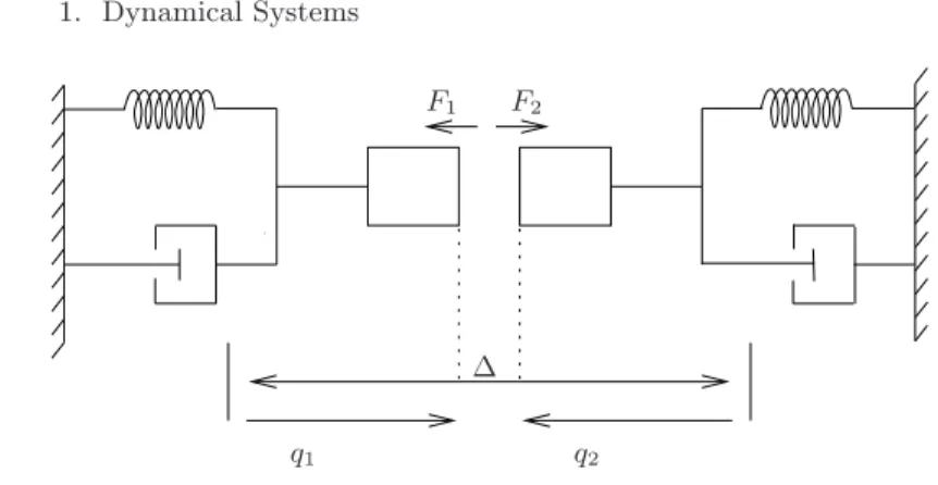
A.3 Autonomous Dynamics of Coupled Masses . . . 396
A.4 Satellite Dynamics . . . 397
A.4.1 Motivation . . . 398
A.4.2 Mathematical modeling . . . 398
A.4.3 Equilibrium Analysis . . . 401
A.4.4 Linearization . . . 401
A.4.5 Analysis of the model . . . 402
A.4.6 Simulation . . . 402
A.5 Dynamics of a Motorbike . . . 402
A.6 Stabilization of a Double Pendulum . . . 404
A.6.1 Modeling . . . 404
A.6.2 Linearization . . . 406
A.6.3 Analysis . . . 407
A.6.4 Stabilization . . . 408
A.7 Notes and References . . . 409
B Background Material 411 B.1 Polynomial Matrices . . . 411
B.2 Partial Fraction Expansion . . . 417
B.3.1 Fourier transform . . . 419
B.3.2 Laplace transform . . . 421
B.4 Notes and References . . . 421
B.5 Exercises . . . 422
Notation 423
References 425
Preface
The purpose of this preface is twofold. Firstly, to give an informal historical introduction to the subject area of this book, Systems and Control, and secondly, to explain the philosophy of the approach to this subject taken in this book and to outline the topics that will be covered.
A brief history of systems and control
Control theory has two main roots:regulationandtrajectory optimization. The first, regulation, is the more important and engineering oriented one. The second, trajectory optimization, is mathematics based. However, as we shall see, these roots have to a large extent merged in the second half of the twentieth century.
The problem of regulation is to design mechanisms that keep certain to-be-controlled variables at constant values against external disturbances that act on the plant that is being regulated, or changes in its properties. The system that is being controlled is usually referred to as theplant, a passe-partout term that can mean a physical or a chemical system, for example. It could also be an economic or a biological system, but one would not use the engineering term “plant” in that case.
x Preface
number of persons present in a room, activity in the kitchen, etc. Motors in washing machines, in dryers, and in many other household appliances are controlled to run at a fixed speed, independent of the load. Modern auto-mobiles have dozens of devices that regulate various variables. It is, in fact, possible to view also the suspension of an automobile as a regulatory device that absorbs the irregularities of the road so as to improve the comfort and safety of the passengers. Regulation is indeed a very important aspect of modern technology. For many reasons, such as efficiency, quality control, safety, and reliability, industrial production processes require regulation in order to guarantee that certain key variables (temperatures, mixtures, pres-sures, etc.) be kept at appropriate values. Factors that inhibit these desired values from being achieved are external disturbances, as for example the properties of raw materials and loading levels or changes in the properties of the plant, for example due to aging of the equipment or to failure of some devices. Regulation problems also occur in other areas, such as economics and biology.
One of the central concepts in control isfeedback:the value of one variable in the plant is measured and used (fed back) in order to take appropriate action through a control variable at another point in the plant. A good example of a feedback regulator is a thermostat: it senses the room temperature, compares it with the set point (the desired temperature), and feeds back the result to the boiler, which then starts or shuts off depending on whether the temperature is too low or too high.
Preface xi
FIGURE P.1. Fly ball governor.
speed changes that would naturally occur in the prime mover when there was a change in the load, which occurred, for example, when a machine was disconnected from the prime mover. Watt’s fly-ball governor achieved this goal by letting more steam into the engine when the speed decreased and less steam when the speed increased, thus achieving a speed that tends to be insensitive to load variations. It was soon realized that this adjustment should be done cautiously, since by overreacting (calledovercompensation), an all too enthusiastic governor could bring the steam engine into oscil-latory motion. Because of the characteristic sound that accompanied it, this phenomenon was called hunting. Nowadays, we recognize this as an instability due to high gain control. The problem of tuning centrifugal gov-ernors that achieved fast regulation but avoided hunting was propounded to James Clerk Maxwell (1831–1870) (the discoverer of the equations for electromagnetic fields) who reduced the question to one about the stability of differential equations. His paper“On Governors,” published in 1868 in theProceedings of the Royal Society of London, can be viewed as the first mathematical paper on control theory viewed from the perspective of reg-ulation. Maxwell’s problem and its solution are discussed in Chapter 7 of this book, under the heading of the Routh-Hurwitz problem.
in-xii Preface
crease when it is too low and decrease when it is too high. The I-term feeds back the integral of the error. This term results in a very large correction signal whenever this error does not converge to zero. For the error there hence holds,Go to zero or bust!When properly tuned, this term achieves
robustness, good performance not only for the nominal plant but also for plants that are close to it, since the I-term tends to force the error to zero for a wide range of the plant parameters. The D-term acts on the derivative of the error. It results in a control correction signal as soon as the error starts increasing or decreasing, and it can thus be expected that this antic-ipatory action results in a fast response. The PID controller had, and still has, a very large technological impact, particularly in the area of chemical process control. A second important event that stimulated the development
ground ampli-fier
V
Vin
Vout
µVout µ= R1
R1+R2
R1
R2
FIGURE P.2. Feedback amplifier.
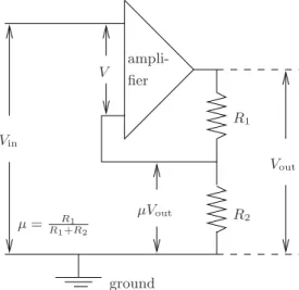
of regulation in the first half of the twentieth century was the invention in the 1930s of the feedback amplifier by Black. The feedback amplifier (see Figure P.2) was an impressive technological development: it permitted sig-nals to be amplified in a reliable way, insensitive to the parameter changes inherent in vacuum-tube (and also solid-state) amplifiers. (See also Exer-cise 9.3.) The key idea of Black’s negative feedback amplifier is subtle but simple. Assume that we have an electronic amplifier that amplifies its input voltage V to Vout =KV. Now use a voltage divider and feed back µVout
to the amplifier input, so that when subtracted (whence the termnegative
feedback amplifier) from the input voltage Vin to the feedback amplifier,
Preface xiii
these two relations yields the crucial formula
Vout= 1
µ+K1 Vin.
This equation, simple as it may seem, carries an important message, see Exercise 9.3.What’s the big deal with this formula? Well, the value of the gainK of an electronic amplifier is typically large, but also very unstable, as a consequence of sensitivity to aging, temperature, loading, etc. The voltage divider, on the other hand, can be implemented by means of pas-sive resistors, which results in a very stable value for µ. Now, for large (although uncertain)Ks, there holds 1
µ+1
K ≈
1
µ, and so somehow Black’s
magic circuitry results in an amplifier with a stable amplification gain 1µ based on an amplifier that has an inherent uncertain gainK.
The invention of the negative feedback amplifier had far-reaching appli-cations to telephone technology and other areas of communication, since long-distance communication was very hampered by the annoying drift-ing of the gains of the amplifiers used in repeater stations. Pursudrift-ing the above analysis in more detail shows also that the larger the amplifier gain K, the more insensitive the overall gain µ+11
K of the feedback amplifier becomes. However, at high gains, the above circuit could become dynam-ically unstable because of dynamic effects in the amplifier. For amplifiers, this phenomenon is calledsinging, again because of the characteristic noise produced by the resistors that accompanies this instability. Nyquist, a col-league of Black at Bell Laboratories, analyzed this stability issue and came up with the celebratedNyquist stability criterion. By pursuing these ideas further, various techniques were developed for setting the gains of feed-back controllers. The sum total of these design methods was termed classi-cal control theoryand comprised such things as the Nyquist stability test, Bode plots, gain and phase margins, techniques for tuning PID regulators, lead–lag compensation, and root–locus methods.
xiv Preface
B A
FIGURE P.3. Brachystochrone.
B A
FIGURE P.4. Cycloid.
Jakob, Leibniz, de l’Hˆopital, Tschirnhaus, and Newton. Newton submit-ted his solution anonymously, but Johann Bernoulli recognized the culprit, since, as he put it,ex ungue leonem: you can tell the lion by its claws.The brachystochrone turned out to be the cycloid traced by a point on the cir-cle that rolls without slipping on the horizontal line throughAand passes through A and B. It is easy to see that this defines the cycloid uniquely (see Figures P.3 and P.4).
The brachystochrone problem led to the development of the Calculus of Variations, of crucial importance in a number of areas of applied mathe-matics, above all in the attempts to express the laws of mechanics in terms of variational principles. Indeed, to the amazement of its discoverers, it was observed that the possible trajectories of a mechanical system are precisely those that minimize a suitable action integral. In the words of Legendre,
Ours is the best of all possible worlds.Thus the calculus of variations had far-reaching applications beyond that of finding optimal paths: in certain applications, it could also tell us what paths are physically possible. Out of these developments came the Euler–Lagrange and Hamilton equations as conditions for the vanishing of the first variation. Later, Legendre and Weierstrass added conditions for the nonpositivity of the second variation, thus obtaining conditions for trajectories to be local minima.
Preface xv
general set of necessary conditions that a control input that generates an optimal path has to satisfy. This result is an important generalization of the classical problems in the calculus of variations. Not only does it allow a much larger class of problems to be tackled, but importantly, it brought forward the problem ofoptimal input selection(in contrast to optimalpath
selection) as the central issue of trajectory optimization.
Around the same time that the maximum principle appeared, it was realized that the (optimal) input could also be implemented as a function of the state. That is, rather than looking for a control input as a function of time, it is possible to choose the (optimal) input as a feedback function of the state. This idea is the basis fordynamic programming, which was formulated by Bellman in the late 1950s and which was promptly published in many of the applied mathematics journals in existence. With the insight obtained by dynamic programming, the distinction between (feedback based)regulation
and the (input selection based)trajectory optimizationbecame blurred. Of course, the distinction is more subtle than the above suggests, particularly because it may not be possible to measure the whole state accurately; but we do not enter into this issue here. Out of all these developments, both in
PLANT
CONTROLLER FEEDBACK
Sensors Actuators
exogenous inputs to-be-controlled outputs
outputs measured inputs
control
FIGURE P.5. Intelligent control.
xvi Preface
objectives, the feedback processor computes what control input to apply. Via the actuators, appropriate influence is thus exerted on the plant. Often, the aim of the control action is to steer the to-be-controlled outputs back to their desired equilibria. This is called stabilization, and will be studied in Chapters 9 and 10 of this book. However, the goal of the controller may also be disturbance attenuation: making sure that the disturbance inputs have limited effect on the to-be-controlled outputs; or it may be
tracking: making sure that the plant can follow exogenous inputs. Or the design question may berobustness: the controller should be so designed that the controlled system should meet itsspecs(that is, that it should achieve the design specifications, as stability, tracking, or a degree of disturbance attenuation) for a wide range of plant parameters.
The mathematical techniques used to model the plant, to analyze it, and to synthesize controllers took a major shift in the late 1950s and early 1960s with the introduction of state space ideas. The classical way of view-ing a system is in terms of the transfer function from inputs to outputs. By specifying the way in which exponential inputs transform into expo-nential outputs, one obtains (at least for linear time-invariant systems) an insightful specification of a dynamical system. The mathematics underly-ing these ideas are Fourier and Laplace transforms, and these very much dominated control theory until the early 1960s. In the early sixties, the prevalent models used shifted from transfer function to state space models. Instead of viewing a system simply as a relation between inputs and out-puts, state space models consider this transformation as taking place via the transformation of the internal state of the system. When state models came into vogue, differential equations became the dominant mathemati-cal framework needed. State space models have many advantages indeed. They are more akin to the classical mathematical models used in physics, chemistry, and economics. They provide a more versatile language, espe-cially because it is much easier to incorporate nonlinear effects. They are also more adapted to computations. Under the impetus of this new way of looking at systems, the field expanded enormously. Important new concepts were introduced, notably (among many others) those ofcontrollabilityand
observability, which became of central importance in control theory. These concepts are discussed in Chapter 5.
Preface xvii
it showed how to compute the feedback control processor of Figure P.5 in order to achieve optimal disturbance attenuation. In this result the plant is assumed to be linear, the optimality criterion involves an integral of a quadratic expression in the system variables, and the disturbances are modeled as Gaussian stochastic processes. Whence the terminology LQG problem. The LQG problem, unfortunately, falls beyond the scope of this introductory book. In addition to being impressive theoretical results in their own right, these developments had a deep and lasting influence on the mathematical outlook taken in control theory. In order to emphasize this, it is customary to refer to the state space theory asmodern control theory
to distinguish it from theclassical control theorydescribed earlier.
Unfortunately, this paradigm shift had its downsides as well. Rather than aiming for a good balance between mathematics and engineering, the field of systems and control became mainly mathematics driven. In particular, mathematical modeling was not given the central place in systems theory that it deserves. Robustness, i.e., the integrity of the control action against plant variations, was not given the central place in control theory that it deserved. Fortunately, this situation changed with the recent formulation and the solution of what is called theH∞problem. TheH∞problem gives a method for designing a feedback processor as in Figure P.5 that is optimally robust in some well-defined sense. Unfortunately, theH∞problem also falls beyond the scope of this introductory book.
A short description of the contents of this book
Both the transfer function and the state space approaches view a system as a signal processor that accepts inputs and transforms them into outputs. In the transfer function approach, this processor is described through the way in which exponential inputs are transformed into exponential outputs. In the state space approach, this processor involves the state as intermediate variable, but the ultimate aim remains to describe how inputs lead to out-puts. This input/output point of view plays an important role in this book, particularly in the later chapters. However, our starting point is different, more general, and, we claim, more adapted to modeling and more suitable for applications.
dy-xviii Preface
namic variables, and it is only when turning to control in Chapters 9 and 10, that we adopt the input/state/output point of view. The general model structures that we develop in the first half of the book are referred to as thebehavioral approach. We now briefly explain the main underlying ideas. We view a mathematical model as a subset of a universum of possibili-ties. Before we accept a mathematical model as a description of reality, all outcomes in the universum are in principle possible. After we accept the mathematical model as a convenient description of reality, we declare that only outcomes in a certain subset are possible. Thus a mathematical model is an exclusion law: it excludes all outcomes except those in a given subset. This subset is called thebehavior of the mathematical model. Proceeding from this perspective, we arrive at the notion of a dynamical system as simply a subset of time-trajectories, as a family of time signals taking on values in a suitable signal space. This will be the starting point taken in this book. Thus the input/output signal flow graph emerges in general as a construct, sometimes a purely mathematical one, not necessarily implying a physical structure.
We take the description of a dynamical system in terms of its behavior, thus in terms of the time trajectories that it permits, as the vantage point from which the concepts put forward in this book unfolds. We are especially interested in linear time-invariant differential systems: “linearity” means that these systems obey thesuperposition principle, “time-invariance” that the laws of the system do not depend explicitly on time, and “differential” that they can be described by differential equations. Specific examples of such systems abound: linear electrical circuits, linear (or linearized) me-chanical systems, linearized chemical reactions, the majority of the models used in econometrics, many examples from biology, etc.
Preface xix
structure of the behavior with free inputs, bound outputs, and the memory, the state variables, is the program of Chapters 3, 4, and 5.
When one models an (interconnected) physical system from first principles, then unavoidably auxiliary variables, in addition to the variables modeled, will appear in the model. Those auxiliary variables are calledlatent vari-ables, in order to distinguish them from themanifest variables, which are the variables whose behavior the model aims at describing. The interaction between manifest and latent variables is one of the recurring themes in this book.
We use this behavioral definition in order to study some important features of dynamical systems. Two important properties that play a central role arecontrollability and observability. Controllability refers to the question of whether or not one trajectory of a dynamical system can be steered towards another one. Observability refers to the question of what one can deduce from the observation of one set of system variables about the behavior of another set. Controllability and observability are classical concepts in control theory. The novel feature of the approach taken in this book is to cast these properties in the context of behaviors.
The book uses the behavioral approach in order to present a systematic view for constructing and analyzing mathematical models. The book also aims at explaining some synthesis problems, notably the design of control algorithms. We treat control from a classical, input/output point of view. It is also possible to approach control problems from a behavioral point of view. But, while this offers some important advantages, it is still a rela-tively undeveloped area of research, and it is not ready for exposition in an introductory text. We will touch on these developments briefly in Section 10.8.
We now proceed to give a chapter-by-chapter overview of the topics covered in this book.
In the first chapter we discuss the mathematical definition of a dynamical system that we use and the rationale underlying this concept. The basic ingredients of this definition are the behavior of a dynamical system as the central object of study and the notions of manifest and latent variables. The manifest variables are what the model aims at describing. Latent variables are introduced as auxiliary variables in the modeling process but are often also introduced for mathematical reasons, for purposes of analysis, or in order to exhibit a special property.
xx Preface
the study of properties of polynomial matrices and their interplay with differential equations.
In the third chapter we study the behavior of linear differential systems in detail. We prove that the variables in such systems may be divided into two sets: one set contains the variables that are free (we call theminputs), the other set contains the variables that are bound (we call themoutputs). We also study how the relation between inputs and outputs can be expressed as a convolution integral.
The fourth chapter is devoted to state models. The state of a dynamical system parametrizes its memory, the extent to which the past influences the future. State equations, that is, the equations linking the manifest variables to the state, turn out to be first-order differential equations. The output of a system is determined only after the input and the initial conditions have been specified.
Chapter 5 deals withcontrollabilityandobservability. A controllable system is one in which an arbitrary past trajectory can be steered so as to be concatenated with an arbitrary future trajectory. An observable system is one in which the latent variables can be deduced from the manifest variables.
These properties play a central role in control theory.
In the sixth chapter we take another look at latent variable and state space systems. In particular, we show how to eliminate latent variables and how to introduce state variables. Thus a system of linear differential equations containing latent variables can be transformed in an equivalent system in which these latent variables have been eliminated.
Stability is the topic of Chapter 7. We give the classical stability conditions of systems of differential equations in terms of the roots of the associated polynomial or of the eigenvalue locations of the system matrix. We also discuss the Routh–Hurwitz tests, which provide conditions for polynomials to have only roots with negative real part.
Up to Chapter 7, we have treated systems in their natural, time-domain setting. However, linear time-invariant systems can also be described by the way in which they process sinusoidal or, more generally, exponential sig-nals. The resulting frequency domain description of systems is explained in Chapter 8. In addition, we discuss some characteristic features and nomen-clature for system responses related to the step response and the frequency domain properties.
Preface xxi
called the pole placement theorem, is one of the central achievements of modern control theory.
The tenth chapter is devoted to observers: algorithms for deducing the sys-tem state from measured inputs and outputs. The design of observers is very similar to the stabilization and pole placement procedures. Observers are subsequently used in the construction of output feedback compensators. Three important cybernetic principles underpin our construction of ob-servers and feedback compensators. The first principle is error feedback:
The estimate of the state is updated through the error between the actual and the expected observations. The second is certainty equivalence. This principle suggest that when one needs the value of an unobserved variable, for example for determining the suitable control action, it is reasonable to use the estimated value of that variable, as if it were the exact value. The third cybernetic principle used is theseparation principle. This implies that we will separate the design of the observer and the controller. Thus the ob-server is not designed with its use for control in mind, and the controller is not adapted to the fact that the observer produces only estimates of the state.
Notes and references
There are a number of books on the history of control. The origins of control, going back all the way to the Babylonians, are described in [40]. Two other his-tory books on the subject, spanning the period from the industrial revolution to the postwar era, are [10, 11]. The second of these books has a detailed account of the invention of the PID regulator and the negative feedback amplifier. A collec-tion of historically important papers, including original articles by Maxwell, Hur-witz, Black, Nyquist, Bode, Pontryagin, and Bellman, among others, have been reprinted in [9]. The history of the brachystochrone problem has been recounted in most books on the history of mathematics. Its relation to the maximum prin-ciple is described in [53]. The book [19] contains the history of the calculus of variations.
There are numerous books that explain classical control. Take any textbook on control written before 1960. The state space approach to systems, and the de-velopment of the LQG problem happened very much under the impetus of the work of Kalman. An inspiring early book that explains some of the main ideas is [15]. The special issue [5] of theIEEE Transactions on Automatic Control con-tains a collection of papers devoted to theLinear–Quadratic–Gaussian problem, up-to-date at the time of publication. Texts devoted to this problem are, for example, [33, 3, 4]. Classical control theory emphasizes simple, but nevertheless often very effective and robust, controllers. Optimal control `a la Pontryagin and LQ control aims at trajectory transfer and at shaping the transient response; LQG techniques center on disturbance attenuation; while H∞ control
empha-sizes regulation against both disturbances and plant uncertainties. The latter,
H∞ control, is an important recent development that originated with the ideas
xxii Preface
1
Dynamical Systems
1.1 Introduction
We start this book at the very beginning, by asking ourselves the question,
What is a dynamical system?
Disregarding for a moment the dynamical aspects—forgetting about time— we are immediately led to ponder the more basic issue, What is a math-ematical model? What does it tell us? What is its mathematical nature? Mind you, we are not asking a philosophical question: we will not engage in an erudite discourse about the relation between reality and its math-ematical description. Neither are we going to elucidate the methodology involved in actually deriving, setting up, postulating mathematical models. What we are asking is the simple question,When we accept a mathematical expression, a formula, as an adequate description of a phenomenon, what mathematical structure have we obtained?
2 1. Dynamical Systems
finished product: it prohibits the creation of finished products unless the required resources are available.
We formalize these ideas by stating that a mathematical model selects a certain subset from a universum of possibilities. This subset consists of the occurrences that the model allows, that it declares possible. We call the subset in question thebehavior of the mathematical model.
True, we have been trained to think of mathematical models in terms of equations.How do equations enter this picture? Simply, an equation can be viewed as a law excluding the occurrence of certain outcomes, namely, those combinations of variables for which the equations are not satisfied. This way, equations define a behavior. We therefore speak of behavioral equa-tionswhen mathematical equations are intended to model a phenomenon. It is important to emphasize already at this point that behavioral equations provide an effective, but at the same time highly nonunique, way of spec-ifying a behavior. Different equations can define the same mathematical model. One should therefore not exaggerate the intrinsic significance of a specific set of behavioral equations.
In addition to behavioral equations and the behavior of a mathematical model, there is a third concept that enters our modeling languageab initio: latent variables. We think of the variables that we try to model asmanifest
variables: they are the attributes on which the modeler in principle focuses attention. However, in order to come up with a mathematical model for a phenomenon, one invariably has to consider other,auxiliary, variables. We call them latent variables. These may be introduced for no other reason than in order to express in a convenient way the laws governing a model. For example, when modeling the behavior of a complex system, it may be convenient to view it as an interconnection of component subsystems. Of course, the variables describing these subsystems are, in general, different from those describing the original system. When modeling the external ter-minal behavior of an electrical circuit, we usually need to introduce the currents and voltages in the internal branches as auxiliary variables. When expressing the first and second laws of thermodynamics, it has been proven convenient to introduce the internal energy and entropy as latent variables. When discussing the synthesis of feedback control laws, it is often impera-tive to consider models that display their internal state explicitly. We think of these internal variables as latent variables. Thus in first principles mod-eling, we distinguish two types of variables. The terminology first principles modeling refers to the fact that the physical laws that play a role in the system at hand are the elementary laws from physics, mechanics, electrical circuits, etc.
1.2 Models 3
properties (such as time-invariance, linearity, stability, controllability, ob-servability) will also refer to the behavior. The subsequent problem then always arises how to deduce these properties from the behavioral equations.
1.2 Models
1.2.1 The universum and the behavior
Assume that we have a phenomenon that we want to model. To start with, we cast the situation in the language of mathematics by assuming that the
phenomenon produces outcomes in a setU, which we call theuniversum. OftenUconsists of a product space, for example a finite dimensional vector space. Now, a (deterministic) mathematical model for the phenomenon (viewed purely from the black-box point of view, that is, by looking at the phenomenon only from its terminals, by looking at the model as descriptive but not explanatory) claims that certain outcomes are possible, while others are not. Hence a model recognizes a certain subsetBofU. This subset is called the behavior (of the model). Formally:
Definition 1.2.1 A mathematical model is a pair (U,B) with U a set, called theuniversum—its elements are called outcomes—andBa subset
ofU, called the behavior.
Example 1.2.2 During the ice age, shortly after Prometheus stole fire from the gods, man realized that H2O could appear, depending on the
temperature, as liquid water, steam, or ice. It took a while longer before this situation was captured in a mathematical model. The generally accepted model, with the temperature in degrees Celsius, isU={ice, water, steam}×
[−273,∞) andB= (({ice} ×[−273,0])∪({water} ×[0,100])∪({steam} ×
[100,∞)).
Example 1.2.3 Economists believe that there exists a relation between the amountP produced of a particular economic resource, the capitalK invested in the necessary infrastructure, and the laborLexpended towards its production. A typical model looks likeU=R3
+ andB ={(P, K, L)∈
R3
+ | P = F(K, L)}, where F : R2+ → R+ is the production function.
Typically,F : (K, L)7→αKβLγ, withα, β, γ∈R
+, 0≤β≤1, 0≤γ≤1,
constant parameters depending on the production process, for example the type of technology used. Before we modeled the situation, we were ready to believe that every triple (P, K, L)∈R3
+ could occur. After introduction of
the production function, we limit these possibilities to the triples satisfying P =αKβLγ. The subset of R3
+ obtained this way is the behavior in the
4 1. Dynamical Systems
1.2.2 Behavioral equations
In applications, models are often described by equations (see Example 1.2.3). Thus the behavior consists of those elements in the universum for which “balance” equations are satisfied.
Definition 1.2.4 LetUbe a universum,Ea set, andf1, f2:U→E. The
mathematical model (U,B) withB={u∈U| f1(u) =f2(u)} is said to be described bybehavioral equations and is denoted by (U,E, f1, f2). The
set E is called the equating space. We also call (U,E, f1, f2) abehavioral
equation representationof (U,B).
Often, an appropriate way of looking atf1(u) = f2(u) is as equilibrium
conditions:the behaviorB consists of those outcomes for which two (sets of) quantities are in balance.
Example 1.2.5 Consider an electrical resistor. We may view this as im-posing a relation between the voltageV across the resistor and the current I through it. Ohm recognized more than a century ago that (for metal wires) the voltage is proportional to the current:V =RI, with the propor-tionality factorR called the resistance. This yields a mathematical model with universumU=R2 and behavior B, induced by the behavioral
equa-tionV =RI. Here E =R, f1 : (V, I)7→V, and f2(V, I) : I 7→RI. Thus
B={(I, V)∈R2
|V =RI}.
Of course, nowadays we know many devices imposing much more com-plicated relations betweenV and I, which we nevertheless choose to call (non-Ohmic) resistors. An example is an (ideal) diode, given by the (I, V) characteristic B = {(I, V) ∈ R2
| (V ≥ 0 and I = 0) or (V = 0 and I≤0)}. Other resistors may exhibit even more complex behavior, due to hysteresis, for example.
Example 1.2.6 Three hundred years ago, Sir Isaac Newton discovered (better: deduced from Kepler’s laws since, as he put it, Hypotheses non fingo) that masses attract each other according to the inverse square law. Let us formalize what this says about the relation between the forceF and the position vector q of the mass m. We assume that the other mass M is located at the origin ofR3. The universumUconsists of all conceivable
force/position vectors, yielding U =R3 ×R3. After Newton told us the
behavioral equations F = −kmM q
1.2 Models 5
R3 | F = −kmM q
kqk3 }, with k the gravitational constant, k = 6.67×10
−8
cm3/g.sec2. Note thatBhas three degrees of freedom–down three from the
six degrees of freedom inU.
In many applications models are described by behavioral inequalities. It is easy to accommodate this situation in our setup. Simply take in the above definition E to be an ordered space and consider the behavioral inequality f1(u) ≤ f2(u). Many models in operations research (e.g., in
linear programming) and in economics are of this nature. In this book we will not pursue models described by inequalities.
Note further that whereas behavioral equations specify the behavior uniquely, the converse is obviously not true. Clearly, if f1(u) = f2(u) is
a set of behavioral equations for a certain phenomenon and iff :E→E′is any bijection, then the set of behavioral equations (f◦f1)(u) = (f◦f2)(u)
form another set of behavioral equations yielding the same mathematical model. Since we have a tendency to think of mathematical models in terms of behavioral equations, most models being presented in this form, it is important to emphasize their ancillary role:it is the behavior, the solution set of the behavioral equations, not the behavioral equations themselves, that is the essential result of a modeling procedure.
1.2.3 Latent variables
Our view of a mathematical model as expressed in Definition 1.2.1 is as follows: identify the outcomes of the phenomenon that we want to model (specify the universum U) and identify the behavior (specify B ⊆ U). However, in most modeling exercises we need to introduce other variables in addition to the attributes inUthat we try to model. We call these other, auxiliary, variableslatent variables. In a bit, we will give a series of instances
where latent variables appear. Let us start with two concrete examples.
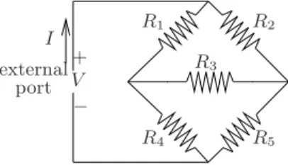
Example 1.2.7 Consider a one-port resistive electrical circuit. This con-sists of a graph with nodes and branches. Each of the branches contains a resistor, except one, which is an external port. An example is shown in Figure 1.1. Assume that we want to model the port behavior, the rela-tion between the voltage drop across and the current through the external port. Introduce as auxiliary variables the voltages (V1, . . . , V5) across and
the currents (I1, . . . , I5) through the internal branches, numbered in the
obvious way as indicated in Figure 1.1. The following relations must be satisfied:
6 1. Dynamical Systems
• Kirchhoff ’s voltage law: the sum of the voltage drops across the branches of any loop must be zero;
• Theconstitutive laws of the resistors in the branches.
I
port external
−
V
R4 R1
R3 R2
R5
+
FIGURE 1.1. Electrical circuit with resistors only.
These yield:
Constitution laws Kirchhoff ’s current laws Kirchhoff ’s voltage laws
R1I1 = V1, I = I1+I2, V1+V4 =V,
R2I2 = V2, I1 = I3+I4, V2+V5 =V,
R3I3 = V3, I5 = I2+I3, V1+V4 =V2+V5,
R4I4 = V4, I = I4+I5, V1+V3 =V2,
R5I5 = V5, V3+V5 =V4.
Our basic purpose is to express the relation between the voltage across and current into the external port. In the above example, this is a relation of the formV =RI(whereRcan be calculated fromR1, R2, R3, R4,andR5),
obtained by eliminating (V1, . . . , V5, I1, . . . , I5) from the above equations.
However, the basic model, the one obtained fromfirst principles, involves the variables (V1, . . . , V5, I1, . . . , I5) in addition to the variables (V, I) whose
behavior we are trying to describe. The node voltages and the currents through the internal branches (the variables (V1, . . . , V5, I1, . . . , I5) in the
above example) are thus latent variables. The port variables (V, I) are the manifest variables. The relation betweenIandV is obtained by eliminating the latent variables. How to do that in a systematic way is explained in
Chapter 6. See also Exercise 6.1.
Example 1.2.8 An economist is trying to figure out how much of a pack-age ofn economic goods will be produced. As a firm believer in equilib-rium theory, our economist assumes that the production volumes consist of those points where, product for product, the supply equals the demand. This equilibrium set is a subset ofRn
+. It is the behavior that we are
1.2 Models 7
n products. Next determine, using economic theory or experimentation, the supply and demand functions Si : Rn+ → R+ and Di : Rn+ → R+.
Thus Si(p1, p2, . . . , pn) and Di(p1, p2, . . . , pn) are equal to the amount of
producti that is bought and produced when the going market prices are p1, p2, . . . , pn. This yields the behavioral equations
si = Si(p1, p2, . . . , pn),
di = Di(p1, p2, . . . , pn),
si = di=Pi, i= 1,2, . . . , n.
These behavioral equations describe the relation between the pricespi, the
suppliessi, the demands di, and the production volumesPi. The Pis for
which these equations are solvable yield the desired behavior. Clearly, this behavior is most conveniently specified in terms of the above equations, that is, in terms of the behavior of the variablespi,si,di, andPi(i= 1,2, . . . , n)
jointly. The manifest behavioral equations would consist of an equation
involvingP1, P2, . . . , Pn only.
These examples illustrate the following definition.
Definition 1.2.9 Amathematical model with latent variables is defined as a triple (U,Uℓ,Bf) withUtheuniversumof manifest variables,Uℓthe
uni-versum oflatent variables, andBf⊆U×Uℓthefull behavior. It defines the
manifest mathematical model(U,B) withB:={u∈U| ∃ℓ∈Uℓsuch that
(u, ℓ)∈Bf}; Bis called the manifest behavior (or the external behavior) or simply thebehavior. We call (U,Uℓ,Bf)a latent variable representation
of (U,B).
8 1. Dynamical Systems
one should not be nonchalant about declaring certain variables measurable and observed. Therefore, we will not further encourage the point of view that identifiesmanifest with observable, andlatent withunobservable. Situations in which basic models use latent variables either for mathematical
reasons or in order to express the basic laws occur very frequently. Let us mention a few:internal voltagesandcurrentsin electrical circuits in order to express the external port behavior;momentumin Hamiltonian mechanics in order to describe the evolution of the position;internal energy andentropy
in thermodynamics in order to formulate laws restricting the evolution of the temperature and the exchange of heat and mechanical work;prices in economics in order to explain the production and exchange of economic goods;state variables in system theory in order to express the memory of a dynamical system; thewave function in quantum mechanics underlying observables; and finally, thebasic probability space Ω in probability theory: the big latent variable space in the sky, our example of a latent variable spacepar excellence.
Latent variables invariably appear whenever we model a system by the method oftearingandzooming. The system is viewed as an interconnection of subsystems, and the modeling process is carried out byzoomingin on the individual subsystems. The overall model is then obtained by combining the models of the subsystems with the interconnection constraints. This ultimate model invariably contains latent variables: the auxiliary variables introduced in order to express the interconnections play this role.
Of course, equations can also be used to express the full behaviorBf of a latent variable model (see Examples 1.2.7 and 1.2.8). We then speak offull behavioral equations.
1.3 Dynamical Systems
We now apply the ideas of Section 1.2 in order to set up a language for dynamical systems. The adjectivedynamical refers to phenomena with a
1.3 Dynamical Systems 9
1.3.1 The basic concept
Definition 1.3.1 Adynamical systemΣ is defined as a triple Σ = (T,W,B),
withTa subset ofR, called the time axis,Wa set called thesignal space, andB a subset ofWT called thebehavior(WT is standard mathematical notation for the collection of all maps fromTtoW).
The above definition will be used as aleitmotivthroughout this book. The set T specifies the set of time instances relevant to our problem. Usually
TequalsRor R+ (incontinuous-time systems),Zor Z+ (indiscrete-time
systems), or, more generally, an interval in RorZ.
The set W specifies the way in which the outcomes of the signals pro-duced by the dynamical system are formalized as elements of a set. These outcomes are the variables whose evolution in time we are describing. In what are called lumped systems, systems with a few well-defined simple components each with a finite number of degrees of freedom,Wis usually a finite-dimensional vector space. Typical examples are electrical circuits and mass–spring–damper mechanical systems. In this book we consider al-most exclusively lumped systems. They are of paramount importance in engineering, physics, and economics. Indistributed systems, Wis often an infinite-dimensional vector space. For example, the deformation of flexible bodies or the evolution of heat in media are typically described by partial differential equations that lead to an infinite-dimensional function spaceW. In areas such as digital communication and computer science, signal spaces
Wthat are finite sets play an important role. WhenW is a finite set, the termdiscrete-event systemsis often used.
In Definition 1.3.1 the behaviorB is simply a family of time trajectories taking their values in the signal space. Thus elements ofBconstitute pre-cisely the trajectories compatible with the laws that govern the system: B consists of all time signals which—according to the model—can conceiv-ably occur, are compatible with the laws governing Σ, while those outside Bcannot occur, are prohibited. The behavior is hence the essential feature of a dynamical system.
Example 1.3.2 According to Kepler, the motion of planets in the solar system obeys three laws:
(K.1) planets move in elliptical orbits with the sun at one of the foci;
(K.2) the radius vector from the sun to the planet sweeps out equal areas in equal times;
10 1. Dynamical Systems
If a definition is to show proper respect and do justice to history, Kepler’s laws should provide the very first example of a dynamical system. They do. TakeT =R(disregarding biblical considerations and modern cosmology: we assume that the planets have always been there, rotating, and will always rotate),W=R3 (the position space of the planets), andB={w:
R→R3| Kepler’s laws are satisfied}. Thus the behaviorBin this example
consists of theplanetary motionsthat, according to Kepler, are possible, all trajectories mapping the time-axisRintoR3 that satisfy his three famous
laws. Since for a given trajectoryw:R→R3one can unambiguously decide
whether or not it satisfies Kepler’s laws,Bis indeed well-defined. Kepler’s laws form a beautiful example of a dynamical system in the sense of our definition, since it is one of the few instances in whichBcan be described explicitly, and not indirectly through differential equations. It took no lesser man than Newton to think up appropriate behavioral differential equations
for this dynamical system.
Example 1.3.3 Let us consider the motion of a particle in a potential fieldsubject to an external force. The purpose of the model is to relate the positionqof the particle inR3to the external forceF. ThusW, the signal
space, equalsR3×R3: three components for the position q, three for the
force F. Let V: R3 →Rdenote the potential field. Then the trajectories
(q, F), which, according to the laws of mechanics, are possible, are those that satisfy the differential equation
md
2q
dt2 +V′(q) =F,
where mdenotes the mass of the particle and V′ the gradient ofV. For-malizing this model as a dynamical system yieldsT=R,W=R3×R3, and
B={(q, F)|R→R3×R3|md2 q
dt2 +V′(q) =F}.
1.3.2 Latent variables in dynamical systems
The definition of alatent variable model is easily generalized to dynamical systems.
Definition 1.3.4 A dynamical system with latent variables is defined as ΣL = (T,W,L,Bf) with T ⊆ R the time-axis, W the (manifest) signal
space,Lthelatent variable space, andBf⊆(W×L)T thefull behavior. It defines a latent variable representation of themanifest dynamical system
Σ = (T,W,B) with (manifest) behavior B := {w : T → W| ∃ ℓ : T →
Lsuch that (w, ℓ)∈Bf}.
1.3 Dynamical Systems 11
system with latent variables each trajectory in the full behaviorBf consists of a pair (w, ℓ) with w:T→Wandℓ :T→L. The manifest signal w is the one that we are really interested in. Thelatent variable signal ℓ in a sense “supports”w. If (w, ℓ)∈Bf, thenw is a possible manifest variable trajectory sinceℓcan occur simultaneously withw.
Let us now look at two typical examples of how dynamical models are constructed from first principles. We will see that latent variables are un-avoidably introduced in the process. Thus, whereas Definition 1.3.1 is a good concept as a basic notion of a dynamical system, typical models will involve additional variables to those whose behavior we wish to model.
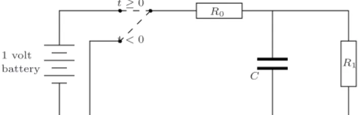
Example 1.3.5 Our first example considers the port behavior of the elec-trical circuit shown in Figure 1.2. We assume that the elementsRC, RL, L,
IRC
IC
−
V
L
V
VRC
VC VRL
VL
−
+
environment
system
RL
I
+
−
RC
C
I
IRL
IL
−
+
−
+ +
− +
FIGURE 1.2. Electrical circuit.
andC all have positive values. The circuit interacts with its environment through the external port. The variables that describe this interaction are the currentI into the circuit and the voltage V across its external termi-nals. These are the manifest variables. Hence W = R2. As time- axis in
this example we takeT=R. In order to specify the port behavior, we in-troduce as auxiliary variables the currents through and the voltages across the internal branches of the circuit, as shown in Figure 1.2. These are the
latent variables. HenceL=R8.
The following equations specify the laws governing the dynamics of this circuit. They define the relations between the manifest variables (the port current and voltage) and the latent variables (the branch voltages and currents). These equations constitute thefull behavioral equations.
Constitutive equations:
VRC =RCIRC, VRL =RLIRL, C dVC
dt =IC, L dIL
12 1. Dynamical Systems
Kirchhoff ’s current laws:
I=IRC+IL, IRC =IC, IL=IRL, IC+IRL =I; (1.2)
Kirchhoff ’s voltage laws:
V =VRC +VC, V =VL+VRL, VRC+VC=VL+VRL. (1.3)
In what sense do these equations specify a manifest behavior? In principle this is clear from Definition 1.3.4. But is there a more explicit way of describing the manifest behavior other than through (1.1, 1.2, 1.3)? Let us attempt to eliminate the latent variables in order to come up with an explicit relation involvingV andIonly. In the example at hand we will do this elimination in an ad hoc fashion. In Chapter 6, we will learn how to do it in a systematic way.
Note first that the constitutive equations (1.1) allow us to eliminateVRC, VRL, IC, andVL from equations (1.2, 1.3). These may hence be replaced by
I=IRC +IL, IRC =C dVC
dt , IL=IRL, (1.4) V =RCIRC +VC, V =L
dIL
dt +RLIRL. (1.5) Note that we have also dropped the equationsIC+IRL =I and VRC + VC =VL+VRL, since these are obviously redundant. Next, use IRL =IL and IRC =
V−VC
RC to eliminateIRL and IRC from (1.4) and (1.5) to obtain
RLIL+L
dIL
dt =V, (1.6)
VC+CRC
dVC
dt =V, (1.7)
I=V −VC RC
+IL. (1.8)
We should still eliminateILandVC from equations (1.6, 1.7, 1.8) in order
to come up with an equation that contains only the variablesV andI. Use equation (1.8) in (1.6) to obtain
VC+
L RL
dVC
dt = (1 + RC
RL
)V + L RL
dV
dt −RcI− LRC
RL
dI
dt, (1.9)
VC+CRC
dVC
dt =V. (1.10)
Next, divide (1.9) by RLL and (1.10) byCRC, and subtract. This yields
(RL L −
1 CRC
)VC= (RC
L +
RL
L − 1 CRC
)V+dV dt −
RCRL
L I−RC dI
1.3 Dynamical Systems 13
Now it becomes necessary to consider two cases:
Case 1: CRC 6= RLL. Solve (1.11) for VC and substitute into (1.10). This
yields, after some rearranging,
(RC RL
+ (1 +RC RL
)CRC
d
dt+CRC L RL
d2
dt2)V = (1 +CRC
d dt)(1 +
L RL
d dt)RCI
(1.12) as the relation betweenV and I.
Case 2: CRC=RLL. Then (1.11) immediately yields
(RC RL
+CRC
d
dt)V = (1 +CRC d
dt)RCI (1.13)
as the relation between V and I. We claim that equations (1.12, 1.13) specify the manifest behavior defined by the full behavioral equations (1.1, 1.2, 1.3). Indeed, our derivation shows that (1.1, 1.2, 1.3) imply (1.12, 1.13). But we should also show the converse. We do not enter into the details here, although in the case at hand it is easy to prove that (1.12, 1.13) imply (1.1, 1.2, 1.3). This issue will be discussed in full generality in Chapter 6. This example illustrates a number of issues that are important in the sequel. In particular:
1. The full behavioral equations (1.1, 1.2, 1.3) are all linear differential equations. (Note: we consider algebraic relations as differential equations of order zero). The manifest behavior, it turns out, is also described by a linear differential equation, (1.12) or (1.13). A coincidence? Not really: in Chapter 6 we will learn that this is the case in general.
2. The differential equation describing the manifest behavior is (1.12) when CRC6= RLL. This is an equation of order two. WhenCRC= RLL, however,
it is given by (1.13), which is of order one. Thus the order of the differen-tial equation describing the manifest behavior turns out to be a sensitive function of the values of the circuit elements.
3. We need to give an interpretation to the anomalous caseCRC= RLL, in the sense that for these values a discontinuity appears in the manifest be-havioral equations. This interpretation, it turns out, isobservability, which
will be discussed in Chapter 5.
Example 1.3.6 As a second example for the occurrence of latent variables, let us consider a Leontieff model for an economy in which several economic goods are transformed by means of a number of production processes. We are interested in describing the evolution in time of the total utility of the goods in the economy. Assume that there are N production processes in whichneconomic goods are transformed into goods of the same kind, and that in order to produce one unit of goodjby means of thekth production process, we need at leastak
14 1. Dynamical Systems
{1,2, . . . , N},i, j∈n:={1,2, . . . , n}, are called thetechnology coefficients. We assume that in each time unit one production cycle takes place. Denote by
qi(t) the quantity of productiavailable at timet
uk
i(t) the quantity of product i assigned to the production process k
at time t, yk
i(t) the quantity of product iacquired from the production process
k at timet. Then the following hold:
n X
k=1
uk
i(t) ≤ qi(t) ∀i∈n,
n X
i=1
ak
ijuki(t) ≥ yjk(t+ 1) ∀k∈N , i∈n,
qi(t) ≤ n X
k=1
yk
i(t) ∀i∈n.
(1.14)
The underlying structure of the economy is shown in Figure 1.3. The differ-ences between the right-hand and left-hand sides of the above inequalities are due to such things as inefficient production, imbalance of the available products, consumption, and other forms of waste. Now assume that the
to-system
u1
i(t);i∈n
process
process 1
k
N
yik(t+ 1);i∈n qi(t+ 1);i∈n
yi1(t+ 1);i∈n
uNi (t);i∈n
qi(t);i∈n uki(t);i∈n
production yN
i (t+ 1);i∈n
production
process production
environment
1.4 Linearity and Time-Invariance 15
tal utility of the goods in the economy is a function of the available amount of goodsq1, q2, . . . , qn; i.e.,J :Z→R+ is given by
J(t) = η(q1(t), . . . , qn(t)),
withη:Rn
+→R+a given function, the utility. For example, if we identify
utility with resale value (in dollars, say), then η(q1, q2, . . . , qn) is equal to Pn
k=1piqi withpi the per unit selling price of goodi.
How does this example fit in our modeling philosophy?
The first question to ask is,What is the time-set? It is reasonable to take
T=Z. This does not mean that we believe that the products have always existed and that the factories in question are blessed with life eternal. What instead it says is that for the purposes of our analysis it is reasonable to assume that the production cycles have already taken place very many times before and that we expect very many more production cycles to come.
The second question is, What are we trying to model?What is our signal space? As die-hard utilitarians we decide that all we care about is the total utilityJ, whence W=R+.
The third question is, How is the behavior defined? This is done by in-equalities (1.14). Observe that these inin-equalities involve, in addition to the manifest variable J, as latent variables the us, qs, and ys. Hence
L=Rn
+×Rn+×m×R n×p + .
The full behavior is now defined as consisting of those trajectories satisfy-ing the behavioral difference inequalities (1.14). These relations define the intrinsic dynamical system withT=Z,W=R+, and the manifest
behav-ior B = {J : Z → R+ | ∃ qi : Z → R+, uki : Z → R+, yki : Z → R+,
i∈n, k ∈N, such that the inequalities (1.14) are satisfied for allt∈Z}. Note that in contrast to the previous example, where it was reasonably easy to obtain behavioral equations (1.12) or (1.13) explicitly in terms of the external attributesV andI, it appears impossible in the present example to eliminate theqs,us, andys and obtain an explicit behavioral equation (or, more likely, inequality) describing B entirely in terms of the J, the
variables of interest in this example.
1.4 Linearity and Time-Invariance
16 1. Dynamical Systems
Definition 1.4.1 A dynamical system Σ = (T,W,B) is said to be linear ifWis a vector space (over a fieldF: for the purposes of this book, think of it asRorC), andBis a linear subspace ofWT(which is a vector space in the obvious way by pointwise addition and multiplication by a scalar).
Thus linear systems obey the superposition principle in its ultimate and very simplest form:{w1(·), w2(·)∈B;α, β∈F} ⇒ {αw1(·) +βw2(·)∈B}.
Time-invariance is a property of dynamical systems governed by laws that do not explicitly depend on time: if one trajectory islegal (that is, in the behavior), then the shifted trajectory is alsolegal.
Definition 1.4.2 A dynamical system Σ = (T,W,B) withT=Zor Ris said to betime-invariantifσtB=Bfor allt∈T(σtdenotes thebackward
t-shift: (σtf)(t′) :=f(t′ +t)). If T= Z, then this condition is equivalent toσB=B. If T=Z+ orR+, then time-invariance requiresσtB⊆Bfor
allt ∈T. In this book we will almost exclusively deal with T= Ror Z, and therefore we may as well think of time-invariance as σtB = B. The
conditionσtB=Bis calledshift-invarianceofB.
Essentially all the examples that we have seen up to now are examples of time-invariant systems.
Example 1.4.3 As an example of a time-varying system, consider the motion of a point-mass with a time-varying mass m(·), for example, a burning rocket. The differential equation describing this motion is given by
d dt(m(t)
d
dtq) =F.
If we view this as a model for the manifest variables (q, F)∈R3×R3, then
the resulting dynamical system is linear but time-varying. If we view this as a model for the manifest variables (q, F, m)∈R3×R3×R
+, then the
resulting dynamical system is time-invariant but nonlinear (see Exercise
1.5).
The notion of linearity and time-invariance can in an obvious way be ex-tended to latent variable dynamical systems. We will not explicitly write down these formal definitions.
1.5 Dynamical Behavioral Equations
1.5 Dynamical Behavioral Equations 17
defined as those elements of this universum satisfying a set of equations, called behavioral equations. In dynamical systems these behavioral equa-tions often take the form of differential equaequa-tions or of integral equaequa-tions. All of our examples have been of this type. Correction: all except Kepler’s laws, Example 1.3.2, where the behavior was described explicitly, although even there one could associate equations to K.1, K.2, and K.3.
We now formalize this. We describe first the ideas in terms of difference equations, since they involve the fewest difficulties of a technical mathemati-cal nature. Abehavioral difference equationrepresentation of a discrete-time dynamical system with time-axisT=Z and signal spaceW is defined by a nonnegative integerL(called thelag, or theorderof the difference equa-tion), a setE(called theequating space), and two mapsf1, f2:WL+1→E,
yielding the difference equations
f1(w, σw, . . . , σL−1w, σLw) =f2(w, σw, . . . , σL−1w, σLw).
Note that this is nothing more than a compact way of writing the difference equation
f1(w(t), w(t+ 1), . . . , w(t+L)) =f2(w(t), w(t+ 1), . . . , w(t+L)).
These equations define the behavior by
B={w:Z→W|f1(w, σw, . . . , σL−1w, σLw) =f2(w, σw, . . . , σL−1w, σLw)}.
In many applications it is logical to consider difference equations that have both positive and negative lags, yielding the behavioral equations
f1(σLminw, σLmin+1w, . . . , σLmaxw) =f2(σLminw, σLmin+1w, . . . , σLmaxw).
(1.15) We callLmax−Lminthelagof this difference equation. We assumeLmax≥
Lmin, but either or both of them could be negative. Whether forward lags
(powers ofσ) or backward lags (powers ofσ−1) are used is much a matter of
tradition. In control theory, forward lags are common, but econometricians like backward lags. The behavior defined by (1.15) is
B={w:Z→W|f1(σLminw, . . . , σLmaxw) =f2(σLminw, . . . , σLmaxw)}.
It is clear that the system obtained this way defines a time-invariant dy-namical system.
Example 1.5.1 As a simple example, consider the following algorithm for computing themoving average of a time-series:
a(t) =
T X
k=−T