FEATURES AND GROUND AUTOMATIC EXTRACTION FROM AIRBORNE LIDAR
DATA
D. Costantino *, M. G. Angelini
DIASS - Faculty Engineering of Taranto, Technical University of Bari - 74123 Taranto, Italy
(d.costantino, mg.angelini)@ poliba.it
Commission VI, WG VI/4
KEY WORDS: LiDAR data, segmentation, building detection, DTM, skewness, kurtosis ABSTRACT:
The aim of the research has been the developing and implementing an algorithm for automated extraction of features from LIDAR scenes with varying terrain and coverage types. This applies the moment of third order (Skweness) and fourth order (Kurtosis). While the first has been applied in order to produce an initial filtering and data classification, the second, through the introduction of the weights of the measures, provided the desired results, which is a finer classification and less noisy. The process has been carried out in Matlab but to reduce processing time, given the large data density, the analysis has been limited at a mobile window. It was, therefore, arranged to produce subscenes in order to covers the entire area. The performance of the algorithm, confirm its robustness and goodness of results. Employment of effective processing strategies to improve the automation is a key to the implementation of this algorithm. The results of this work will serve the increased demand of automation for 3D information extraction using remotely sensed large datasets. After obtaining the geometric features from LiDAR data, we want to complete the research creating an algorithm to vector features and extraction of the DTM.
* Corresponding author. This is useful to know for communication with the appropriate person in cases with more than one author. 1. INTRODUCTION
1.1 General introduction
The LiDAR survey has the main advantage to provide a direct method for 3D data collection,infact, it directly collects an accurately georeferenced set of dense point clouds, which can be almost directly used in basic applications. However, the full exploitation of LiDAR’s potentials and capabilities challenges for new data processing methods that are fundamentally different from the ones used in traditional photogrammetry. Over the last decade, there have been many significant developments in this filed, mainly resulting from multidisciplinary research, including computer vision, computer graphics, electrical engineering and photogrammetry. Extracting thematic features, including road, building and vegetation, from these 3D point clouds are paid much attention recently. The processing of LiDAR data is still in an early phase of development although LiDAR systems are already in a mature state (Flood, 2001). Existing algorithms often exploit only part of information contained in LiDAR data, or just focus on processing specific scenes, for example, urban or forested areas. The penetrable vegetation or solid surfaces can be detected if multi-return LiDAR range data are available (Kraus et al. 2001). DTM generation is among one of the most direct applications for LiDAR data processing. Because the sampled LiDAR points are collected from the top of the Earth’s surface partly covered by aboveground features, the DTM generation needs to identify the terrain points on the bare earth, and to remove non-terrain points hit on trees, buildings and other constructions based on terrain points. In academic community, many algorithms have been developed to process relatively flat, urban, forested, mountainous areas, or in a few cases, hybrid areas (Weidner and Forstner, 1995; Axelsson, 1999). However, these algorithms usually use single-return range data only, and omit the valuable information contained in multi-return range data or intensity data. However, researchers have to customize
different versions of these algorithms for different situations. In industry community, the adaptive filtering algorithm based on TINs was developed by Axelsson (2000), and has been implemented in the commercial software TerraScanTM from TerraSolid (2001). But, the production procedure needs interactive inputs from operators, and heavily depends on manual operations to generate high-quality DTMs. LiDAR data contains much 3D information about buildings. But buildings are highly unstructured segments with very complex contents and elevation variations in range data. Buildings can be located at any places, and may be surrounded by other objects with similar radiometric properties in intensity such as roads. The geometric resolution of LiDAR data may be limited due to irregular sampling patterns, and tall trees may occlude parts of building or house roofs in densely vegetated and built-up areas. Many algorithms focus on the detection of building footprints because the reconstruction of complex building roofs in 3D is very difficult (Baltsavias et al., 1999). The use of LiDAR intensity or range data can benefit the separation of buildings and vegetation ( Brunn and Weidner, 1998; Elberink and Maas, 2000; Hofmann, 2001). But building footprints cannot be detected fully automatically and reliably and are often assumed to be of simple shapes with orthogonal corners such as rectangles or low- quality polygons (Weidner, 1995; Vosselman, 1999). The reconstruction of 3D building models is more difficult and is often limited to simple and specific cases assuming rectilinear footprints, parametric shapes, flat or symmetric sloped roofs (Weidner and Forstner, 1995; Lin et al. 2008; Maas and Vosselman, 1999; Vosselman, 1999; Vosselman and Dijkman, 2001; Elaksher and Bethel, 2002). 1.2 Area test and Dataset
The Oria data set provided by Geocart s.r.l. Engineering Company The equipment included a RIEGL LMS-Q560 laser scanner. The instrument makes use of the time-of-flight distance measurement principle of nanosecond infrared pulses. Fast opto-mechanical beam scanning provides absolutely linear,
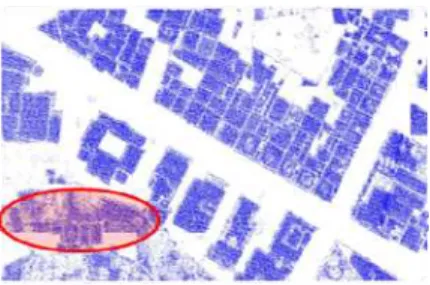
unidirectional and parallel scan lines. The instrument is extremely rugged, therefore ideally suited for the installation on aircraft. Also, it is compact and lightweight enough to be installed in small twin- or single-engine planes, helicopters or UAVs. The range and intensity images have a spatial resolution of 0.15 m. The data are in UTM33, based on the WGS84 coordinate system. The data files are in simple LAS format with three ground coordinates and intensity values. The data sets have been processed with the hierarchical approach of the filter algorithm described above. Default values have been used for the parameters of the filter and no manual editing was performed. Tuning the parameters might have improved the result slightly but at the expense of more time spent. First, all strips were combined to one file. We used the whole data set (16717951 pts), which contains all the recorded echoes (pulses), because our aim was to filter the vegetation and houses and obtain a ground model. The covered area is ~ 600 m for ~ 600 m and for practical reasons the Oria dataset was split in four areas. The amount of information contained in such high-density 3D point clouds is enormous. Only two parts has been treated in more detail. The size of these sample areas are 19600 m2 (Area Test I) and 13500 m2 (Area Test II) (figure 1).
Figure 1 - LiDAR dataset: Area test I and Area test II The Area Test I is a typical suburban area with large terrain relief. Dense trees cover most area since the data was acquired in summer. In the center, there is the castle. At the east part, there are hills with large undulations, so this scene has high complexity. The Area Test II scene is a typical urban scene. This study area has relatively gentle variations in elevation, almost a relatively flat urban region. There are many small to large buildings, but few trees and cars on roads, the houses are larger but lower than the trees, and the buildings and trees are loosely sited. So this scene has medium complexity. As it can be seen (a small parts of the whole area, which can be seen in the left upper side of figure 1) there is a good mixture of ground and off-terrain points, including especially points on building roofs but also vegetation points (houses, vegetation and negative gross errors which have to be eliminated from the data set). The average point density is 50 pts/mq. The Area Test I is a typical suburban area with large terrain relief. Dense trees cover most area since the data was acquired in summer. In the center, there is the castle. At the east part, there are hills with large undulations, so this scene has high complexity. The Area Test II scene is a typical urban scene. This study area has relatively gentle variations in elevation, almost a relatively flat urban region. There are many small to large buildings, but few trees and cars on roads, the houses are larger but lower than the trees, and the buildings and trees are loosely sited. So this scene has medium complexity.
1.3 Elaboration with SCOP++ and DTMaster
The raw LiDAR points for Area Test have been processed with SCOP++ and classified into five classes, including bare surface
(brown), building (cyan) and high, medium and low vegetation (green). Analysis of results suggests a misclassification for building points, problems for attached to building vegetation and for very steep profile terrain (figure 2).
Figure 2 – SCOP++ Area test I
DTMaster was used to improving the results gotten by SCOP++ or rather has been used to manual edit and refine the output of SCOP++ elaboration. Within DTMaster, it is possible to work on top, perspective or profile views. Figure 3 show the results obtained for Area test I. Each of them required more than two full days of work, despite their small area and there are present not so many buildings.
Figure 3 - DTMaster Area test I
2. EXPERIMENTAL ALGORITHM DEVELOPED
2.1 Developed Algorithm
The approach adopted addresses the separation of ground and object points in LiDAR data according to the following definitions. Ground points include the top layer soil, thin man-made layering such as asphalt or tarmac as defined as bare earth in (Sithole and Vosselman, 2003). At this stage, grass and very low vegetation are also considered as ground points. Object points including detached objects (buildings, trees and bushes) and attached objects (bridges and ramps) as described in (Sithole and Vosselman, 2003) are segmented, too. Data set used, has been provided in LAS format, so it was necessary to use Terrascan software, to convert LAS file in to a MATLAB recognizable format such as TXT. The proposed algorithm works on balancing the distribution of points in LiDAR data. Statistical measures of distribution are independent from the relative position of the points. That is why they do not have to be regularly arranged in a DSM. Therefore, the proposed technique works also on raw point clouds. As kurtosis and
skewness both express the characteristics of the point cloud distribution, they can equally be treated as termination criteria in a segmentation algorithm. In this unsupervised segmentation algorithm, skewness is chosen as a measure to describe the point cloud distribution. This algorithm, shown in figure 4, works as follows: first, the skewness of the point cloud is calculated; if it is greater than zero, peaks dominate the point cloud distribution; thus, the highest value of the point cloud is removed by classifying it as an object point; to separate all ground and object points, these steps are iteratively executed while the skewness of the point cloud is greater than zero; the remaining points in the point cloud finally belong to the ground.
Figure 4 – LiDAR data extraction
The algorithm is divided into four steps. The first step allows us to crop a portion of user-defined area then which performs the
processing. The cutting is done by choosing the dimension of window (in this paper 15x15 or 30x30) and choosing, here, the element i-th and j-th belonging to the dataset matrix to the corresponding area test. The second step performs the data analysis and determines the estimated parameters, the third step performs, based on the parameter skewness calculated in the previous step, the separation between ground points and object points.
1
)
(
1
33
−
−
=
∑
N
z
z
SK
i iσ
(1)where: SK=Skewness;
z
i=altimetric coord.;z
=mean zi;σ
=standard deviation.The skewness (1) shows any asymmetry, if the mean of cubic residual is positive means that the distribution has a tail to the “right” (for values greater than the mean), otherwise it has a negative tail to the left. In order to obtain a measure of asymmetry with which to compare distributions that span several orders of magnitude and not depend on the unit of measurement used, is convenient to express the mean of the cubes of residuals in a unit that is “natural “ distribution of interest. This scale is a natural choice to be the cube of the standard deviations.
Finally, the fourth step allows, based on kurtosis (2) and through the introduction of the weights of the measures, to obtain the desired results, which is a finer classification and less noisy.
4
4
)
(
σ
∑
−
=
kw
kz
kz
PKU
(2)where KU=kurtosis;
w
k=weight;z
P=weighted mean. The latest measure executed, kurtosis, indicates the sharpness of the distribution, or rather if the shape is more reminiscent of a sharp peak “or” a kind of “plateau” (apart from the obvious “irregularities'') has been built from a weighted mean of the fourth degree of the residuals, properly scaled to the fourth power of the standard deviation. The choice of weights has been properly assessed on the basis of minimum value certainly belonging to the ground by introducing a discretization in bands decreased with weight up, or rather to the increasing distance from the presumed location of the ground. The determination of weights is directly related to the average slope of the data sets investigated, using a principle of polynomial interpolation. 2.1.1 ResultsResults for same defined region of the Area Test I and Area Test II are depicted in figure 5 and 6 (with legend bars measured in meters) with the purpose to show how the analysis of the skewness parameter is effective for classification in Terrain and Off-terrain points. The following figures shows several example of the result gotten by the developed Matlab code. Figure 5 (sx) represents a sub-region (15x15 mq) of the Area Test I, where it is possible to distinguish a building façade, the road and two tall trees. Figure 5 (dx) shows the relative point cloud in false colors representing the skewness distribution. Figures 6 show a window 15x15 mq, in perspective view, of the last echo DSM of a portion of the Area Test II, with characteristics of urban area with buildings of different
height and the ground (road) and the relative skewness distribution.
Figure 5 – Area Test I - Window 15x15 mq: (sx) Raw point cloud; (dx) Skewness distribution
Figure 6 – Area Test II - Window 15x15 mq: (sx) Raw point cloud; (dx) Skewness distribution
Figure 7 –- Window 15x15 mq Terrain (yellow) vs. Off-Terrain (red) points distribution: Area Test I (sx); Area Test II (dx) Using the skewness algorithm object and ground points, respectively red and yellow, have been separated as depicted in figure 7. In particular, is show the point clouds classified in the two class Terrain (yellow) and Off-Terrain (red) points for each area test. Using the kurtosis algorithm has been possible to obtain, relatively to the ground points, a clear reduction of noise (figure 8) and the emphasis of the ground (figure 9). In particular, the comparison of the figures 9 and 10, for the same subscene, shows the goodness and the efficiency of the implementation of kurtosis.
Figure 8 – Area Test II - Window 15 m x 15 m, Kurtosis: (sx) Noise distribution top view; (dx) Noise distribution perspective view
Figure 9 – Area Test II - Window 15 m x 15 m, Kurtosis: (sx) Terrain points distribution top view; (dx) Terrain points distribution perspective view
Figure 10 – Area Test II - Window 15 m x 15 m, Skewness: (sx) Terrain points distribution top view; (dx) Terrain points distribution perspective view
2.2 Roofs Extraction
The next step has been the extraction of buildings between the Object points. To this end, it was executed the RANSAC algorithm to detect plans (flat roof and roof pitch of buildings). The RANSAC algorithm (RANdom Sample And Consensus) was first introduced by Fischler and Bolles in 1981 as a method to estimate the parameters of a certain model starting from a set of data contaminated by large amounts of outliers. Despite many modifications, the RANSAC algorithm is essentially composed of two steps that are repeated in an iterative fashion (hypothesize-and-test framework):
1. Hypothesize. First minimal sample sets (MSSs) are randomly selected from the input dataset and the model parameters are computed using only the elements of the MSS. The cardinality of the MSS is the smallest sufficient to determine the model parameters (as opposed to other approaches, such as least squares, where the parameters are estimated using all the data available, possibly with appropriate weights).
2. Test. In the second step RANSAC checks which elements of the entire dataset are consistent with the model instantiated with the parameters estimated in the first step. The set of such elements is called consensus set (CS).
RANSAC terminates when the probability of finding a better ranked CS drops below a certain threshold. In the original formulation the ranking of the CS was its cardinality (i.e. CSs that contain more elements are ranked well than CSs that contain fewer elements). RANSAC.m is the driver function that implements the RANSAC algorithm in MATLAB. It is possible to utilize RANSAC to identify points in R3 that belong to a plane in the space (i.e. to an affine linear manifold in R3) and simultaneously estimate the parameters of such manifold. Figure 11 and figure 12 show the results for the whole Area Test I and Area Test II, respectively. The LiDAR points hit on a building’s roof are retrieved from the raw LiDAR points by doing RANSAC test. At this point, a building model consists of a number of roof points, which can be triangulated to give a
rough delineation of the whole outer surface of a building including its footprint, roof and walls.
.(a) (b)
Figure 11 – Area Test I: (a) Terrain (yellow) vs. Off-Terrain (red) points distribution top view; (b) Roof points detected top view
(a) (b)
(c)
Figure 12 – Area Test II: (a) Raw point cloud (viewed by intensity value); (b) Terrain (yellow) vs. Off-Terrain (red) points distribution top view; (c) Roof points detected top view TIN is widely used to model surfaces. A building was triangulated in 2D and was then visualized in 3D as shown in figure 13 (a). However, this kind of approximation still exhibits too many vertices and facets, and their direct use in GIS will lead to inefficient manipulations. To represent the building’s surface, we remove redundant edges, a part of which are outside the polygon in 2D. Figure 13 (b) shows the corresponding constrained 3D model representation.
(a) (b)
Figure 13 – Triangulated building surface models: (a) TINs of building surface points; (b) Constrained 3D Model
The results obtained have shown a clear separation of detached and most of the attached objects from the ground. Applying RANSAC algorithm for the identification of plans, finally allowed the detection and extraction of the points making up the roofs of buildings. Quantities and quality measures are
performed for above building extraction results. These building models were compared with their corresponding patterns in the orthophoto or CTR shape file (figures 14-15).
(a) (b)
(c) (d)
Figure 14 – Area Test I: (a) Orthophoto; (b) CTR shape file; (c) Roof points detected; (d) Overlay
The rule for determining a match is that the polygon model has an overlap larger than about 75% with the observed building patterns. The buildings sited on the boundaries of the study areas are not counted since it is difficult to detect them due to the shortage of complete information.
(a) (b)
(c) (d)
Figure 15 – Area Test II: (a) Orthophoto; (b) CTR shape file; (c) Roof points detected; (d) Overlay
The building extraction results for the two Area Test I and Area Test II are very good since this scene is of high and medium complexity. The completeness and correctness are as high as 95% and 88%, for the Area Test I and are 93% and 87%, for the Area Test II, respectively. Very few vegetation objects are classified as buildings. The vegetated objects are identified correctly either by shape measures or by the removal of small objects. One of the parameters that most affects the results in the roof points extraction is the size of the moving window (figure 16). Indeed, for small size (i.e.1 m) there could be a Non-ground points over-classification, while for large size (i.e. 50 m) there could be a Ground points over-classification. However, some classification errors can be detected in the
presence of land with slopes very high since, under these conditions, the geometric features of the ground are too similar to those of buildings (figure 17).
Figure 16 – Biases in Roof points detection due to moving window size
Figure 17 – Biases for very steep terrain 3. CONCLUSIONS AND FUTURE PERSPECTIVES
In this work, an automated, robust and efficient algorithm for building and ground extraction from LiDAR data is presented. Working on the original, un-gridded point cloud, measures of distribution have been used to characterize the point cloud distribution and subsequently to filter it. The skewness algorithm has implemented for object and ground point separation. The results presented have shown a clear separation of detached and most of the attached objects from the ground. The fourth step, or rather, the kurtosis has improved the results obtained with the skweness relative to the ground, giving more realistic results. Furthermore, applying the RANSAC algorithm, has been identified the plans for coverage of buildings. The results presented have shown that the proposed algorithm is robust and has potential commercial applications since it is efficient and straightforward to Implement, compared to software SCOP + + and DTMaster that, even though they produce good results, required considerable manual intervention. However, the implementation of the algorithm in matalab, that present the same results for the 15x15 and 30x30 windows, require significant processing time, about 1500 pts/sec and 800 pts/sec.
For future work, the algorithm will be extended to other datasets and to even more complex scenes in order to make it robust, also, against very sloped areas. The algorithm will be written in another programming language in order to obtain major processing speed. The issue of detecting all attached objects will be addressed, too. It is also planned for further research to classify the detected object points (attached and detached objects) into finer categories, it will be taken into account the investigation on the intensity data.
4. REFERENCES AND BIBLIOGRAPHY
References from Journals:
Axelsson P., 1999. Processing of laser scanner data-algorithms and applications. ISPRS Journal of Photogrammetry and Remote Sensing, 54 (2-3), pp. 138-147.
Brunn A., Weidner U., 1998. Hierarchical Bayesian nets for building extraction using dense digital surface models. ISPRS Journal of Photogrammetry and Remote Sensing, 53(5), pp. 296-307.
Elasksher A.F., Bethel J.S., 2002. Reconstructing 3D building from LiDAR data. International Archives of Photogrammetry, Remote Sensing and Spatial Information Sciences, 34(3A), pp. 102-107.
Elberink S. O., Maas H. G., 2000. The use of anisotropic height texture measures for the segmentation of airborne laser scanner data. International Archives of the Photogrammetry and Remote Sensing, Vol. XXXIII Part B3/2, pp. 678.
Flood M., 2001. LiDAR activities and research priorities in the commercial sector. International Archives of Photogrammetry and Remote Sensing, Vol. 34- 3/W4, pp. 3-7.
Maas H.G., Vosselman G., 1999. Two algorithms for extracting building models from raw laser altimetry data. ISPRS Journal of Photogrammetry and Remote Sensing, 54(2-3), pp. 153-163. Vosselman G., Dijkman S., 2001. 3D building model reconstruction from point clouds and ground plans.
International Archives of Photogrammetry, Remote Sensing and Spatial Information Sciences, 34(3W4), pp. 37-43.
References from Other Literature:
Hofmann A., Maas H.G., Streilein A., 2001. Knowledge-based building detection based on laser scanner data and topographic map information, in Proceedings of the ISPRS WG III/3 Workshop, ‘3D Reconstruction from Airborne Laser scanner and InSAR Data’, Dresden, Germany, 2003.
Kraus K., Pfeifer N., 2001. Advanced DTM generation from LiDAR data. IAPRS XXXIV 3/W4, Annapolis, MD.
Lin H., Jing H.T., Zhang L.P., 2008. Fast reconstruction of three dimensional city model based on airborne LiDAR. The international archives of the photogrammetry, remote sensing and spatial information sciences - XXI Congress - Proceedings Vol. XXXVII, pp. 453-458.
Bartels Marc, Hong Wei, David C., 2006 Mason. Generazione di DTM da dati LIDAR con bilanciamento asimmetria. In Atti del CIPR (1), pp.566-569.
Sithole G., Vosselman G., 2003. Comparison of filtering algorithms. Workshop on 3-D reconstruction from airborne laserscanner and InSAR data, October 8-10, 2003, Dresden, Germany. Vol. XXXIV Part 3/W13, ISSN 1682-1777, pp. 71-78.
Weidner U., Förstner W, 1995. Model-Based 2D-Shape Recovery. DAGM- Symposium 1995: pp. 260-268.
5. ACKNOWLEDGEMENTS
Faculty of Engineering of Taranto – Technical University of Bari for the contribution “Fondi Provincia di Taranto 2011”.